数学代写|线性代数代写linear algebra代考|MTH2106
如果你也在 怎样代写线性代数linear algebra这个学科遇到相关的难题,请随时右上角联系我们的24/7代写客服。
线性代数是平坦的微分几何,在流形的切线空间中服务。时空的电磁对称性是由洛伦兹变换表达的,线性代数的大部分历史就是洛伦兹变换的历史。
statistics-lab™ 为您的留学生涯保驾护航 在代写线性代数linear algebra方面已经树立了自己的口碑, 保证靠谱, 高质且原创的统计Statistics代写服务。我们的专家在代写线性代数linear algebra代写方面经验极为丰富,各种代写线性代数linear algebra相关的作业也就用不着说。
我们提供的线性代数linear algebra及其相关学科的代写,服务范围广, 其中包括但不限于:
- Statistical Inference 统计推断
- Statistical Computing 统计计算
- Advanced Probability Theory 高等概率论
- Advanced Mathematical Statistics 高等数理统计学
- (Generalized) Linear Models 广义线性模型
- Statistical Machine Learning 统计机器学习
- Longitudinal Data Analysis 纵向数据分析
- Foundations of Data Science 数据科学基础
数学代写|线性代数代写linear algebra代考|The Dimension of a Subspace
It can be shown that if a subspace $H$ has a basis of $p$ vectors, then every basis of $H$ must consist of exactly $p$ vectors. (See Exercises 27 and 28 .) Thus the following definition makes sense.
The dimension of a nonzero subspace $H$, denoted by $\operatorname{dim} H$, is the number of vectors in any basis for $H$. The dimension of the zero subspace ${0}$ is defined to be zero. ${ }^2$
The space $\mathbb{R}^n$ has dimension $n$. Every basis for $\mathbb{R}^n$ consists of $n$ vectors. A plane through 0 in $\mathbb{R}^3$ is two-dimensional, and a line through $\mathbf{0}$ is one-dimensional.
EXAMPLE 2 Recall that the null space of the matrix $A$ in Example 6 in Section $2.8$ had a basis of 3 vectors. So the dimension of $\operatorname{Nul} A$ in this case is 3 . Observe how each basis vector corresponds to a free variable in the equation $A \mathbf{x}=\mathbf{0}$. Our construction always produces a basis in this way. So, to find the dimension of $\mathrm{Nul} A$, simply identify and count the number of free variables in $A \mathbf{x}=\mathbf{0}$.
The rank of a matrix $A$, denoted by rank $A$, is the dimension of the column space of $A$.
Since the pivot columns of $A$ form a basis for $\operatorname{Col} A$, the rank of $A$ is just the number of pivot columns in $A$.
The row reduction in Example 3 reveals that there are two free variables in $A \mathbf{x}=\mathbf{0}$, because two of the five columns of $A$ are not pivot columns. (The nonpivot columns correspond to the free variables in $A \mathbf{x}=\mathbf{0}$.) Since the number of pivot columns plus the number of nonpivot columns is exactly the number of columns, the dimensions of Col $A$ and $\mathrm{Nul} A$ have the following useful connection. (See the Rank Theorem in Section $4.6$ for additional details.)
The Rank Theorem
If a matrix $A$ has $n$ columns, then $\operatorname{rank} A+\operatorname{dim} \operatorname{Nul} A=n$.
The following theorem is important for applications and will be needed in Chapters 5 and 6. The theorem (proved in Section 4.5) is certainly plausible, if you think of a $p$-dimensional subspace as isomorphic to $\mathbb{R}^p$. The Invertible Matrix Theorem shows that $p$ vectors in $\mathbb{R}^p$ are linearly independent if and only if they also span $\mathbb{R}^p$.
数学代写|线性代数代写linear algebra代考|Column Space and Null Space of a Matrix
Subspaces of $\mathbb{R}^n$ usually occur in applications and theory in one of two ways. In both cases, the subspace can be related to a matrix.
The column space of a matrix $A$ is the set $\operatorname{Col} A$ of all linear combinations of the columns of $A$.
If $A=\left[\begin{array}{lll}\mathbf{a}_1 & \cdots & \mathbf{a}_n\end{array}\right]$, with the columns in $\mathbb{R}^m$, then $\operatorname{Col} A$ is the same as Span $\left{\mathbf{a}_1, \ldots, \mathbf{a}_n\right}$. Example 4 shows that the column space of an $\boldsymbol{m} \times \boldsymbol{n}$ matrix is a subspace of $\mathbb{R}^m$. Note that $\operatorname{Col} A$ equals $\mathbb{R}^m$ only when the columns of $A$ span $\mathbb{R}^m$. Otherwise, $\operatorname{Col} A$ is only part of $\mathbb{R}^m$.
EXAMPLE 4 Let $A=\left[\begin{array}{rrr}1 & -3 & -4 \ -4 & 6 & -2 \ -3 & 7 & 6\end{array}\right]$ and $\mathbf{b}=\left[\begin{array}{r}3 \ 3 \ -4\end{array}\right]$. Determine whether $\mathbf{b}$ is in the column space of $A$.
SOLUTION The vector $\mathbf{b}$ is a linear combination of the columns of $A$ if and only if $\mathbf{b}$ can be written as $A \mathbf{x}$ for some $\mathbf{x}$, that is, if and only if the equation $A \mathbf{x}=\mathbf{b}$ has a solution. Row reducing the augmented matrix $\left[A \begin{array}{ll}A & \mathbf{b}\end{array}\right]$,
$$
\left[\begin{array}{rrrr}
1 & -3 & -4 & 3 \
-4 & 6 & -2 & 3 \
-3 & 7 & 6 & -4
\end{array}\right] \sim\left[\begin{array}{rrrr}
1 & -3 & -4 & 3 \
0 & -6 & -18 & 15 \
0 & -2 & -6 & 5
\end{array}\right] \sim\left[\begin{array}{rrrr}
1 & -3 & -4 & 3 \
0 & -6 & -18 & 15 \
0 & 0 & 0 & 0
\end{array}\right]
$$
we conclude that $A \mathbf{x}=\mathbf{b}$ is consistent and $\mathbf{b}$ is in $\operatorname{Col} A$.
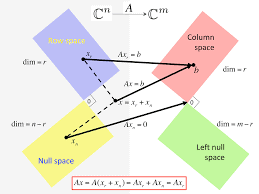
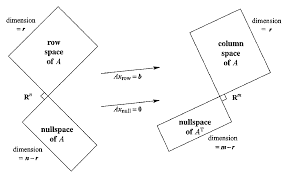
The solution of Example 4 shows that when a system of linear equations is written in the form $A \mathbf{x}=\mathbf{b}$, the column space of $A$ is the set of all $\mathbf{b}$ for which the system has a solution.
The null space of a matrix $A$ is the set $\mathrm{Nul} A$ of all solutions of the homogeneous equation $A \mathbf{x}=\mathbf{0}$
When $A$ has $n$ columns, the solutions of $A \mathbf{x}=\mathbf{0}$ belong to $\mathbb{R}^n$, and the null space of $A$ is a subset of $\mathbb{R}^n$. In fact, $\mathrm{Nul} A$ has the properties of a subspace of $\mathbb{R}^n$.
The null space of an $m \times n$ matrix $A$ is a subspace of $\mathbb{R}^n$. Equivalently, the set of all solutions of a system $A \mathbf{x}=\mathbf{0}$ of $m$ homogeneous linear equations in $n$ unknowns is a subspace of $\mathbb{R}^n$.
PROOF The zero vector is in $\operatorname{Nul} A$ (because $A 0=0$ ). To show that $\mathrm{Nul} A$ satisfies the other two properties required for a subspace, take any $\mathbf{u}$ and $\mathbf{v}$ in $\mathrm{Nul} A$. That is, suppose $A \mathbf{u}=\mathbf{0}$ and $A \mathbf{v}=\mathbf{0}$. Then, by a property of matrix multiplication,
$$
A(\mathbf{u}+\mathbf{v})=A \mathbf{u}+A \mathbf{v}=\mathbf{0}+\mathbf{0}=\mathbf{0}
$$
Thus $\mathbf{u}+\mathbf{v}$ satisfies $A \mathbf{x}=\mathbf{0}$, and so $\mathbf{u}+\mathbf{v}$ is in $\operatorname{Nul} A$. Also, for any scalar $c, A(c \mathbf{u})=$ $c(A \mathbf{u})=c(0)=\mathbf{0}$, which shows that $c \mathbf{u}$ is in $\mathrm{Nul} A$.
To test whether a given vector $\mathbf{v}$ is in $\operatorname{Nul} A$, just compute $A \mathbf{v}$ to see whether $A \mathbf{v}$ is the zero vector. Because $\mathrm{Nul} A$ is described by a condition that must be checked for each vector, we say that the null space is defined implicitly. In contrast, the column space is defined explicitly, because vectors in Col A can be constructed (by linear combinations) from the columns of $A$. To create an explicit description of $\mathrm{Nul} A$, solve the equation $A \mathbf{x}=\mathbf{0}$ and write the solution in parametric vector form. (See Example 6 , below.) ${ }^2$
线性代数代考
数学代写|线性代数代写linear algebra代考|The Dimension of a Subspace
可以证明,如果一个子空间 $H$ 有一个基础 $p$ 向量,然后是的每个基础 $H$ 必须完全由 $p$ 载体。(见刃题 27 和 28。)因此下面的定义是有道理的。
非零子空间的维数 $H$ ,表示为 $\operatorname{dim} H$ ,是任何基础上的向量数 $H$. 零子空间的维数 0 被定义为零。 ${ }^2$ 空间 $\mathbb{R}^n$ 有维度 $n$. 每个基础 $\mathbb{R}^n$ 由组成 $n$ 载体。通过 0 英寸的平面 $\mathbb{R}^3$ 是二维的,一条线穿过 $\mathbf{0}$ 是一维的。
示例 2 回想一下矩阵的零空间 $A$ 在示例 6 中 $2.8$ 有3个向量的基础。所以维度 $\mathrm{Nul} A$ 在这种情况下是 3 。 观察每个基向量如何对应于方程中的一个自由变量 $A \mathbf{x}=\mathbf{0}$. 我们的建设总是以这种方式产生基础。所 以,要找到的维度 $\mathrm{Nul} A$ ,简单地识别和计算自由变量的数量 $A \mathbf{x}=0$.
矩阵的秩 $A$ ,用秩表示 $A$, 是列空间的维数 $A$.
由于枢轴列 $A$ 打下基础 $\operatorname{Col} A$ ,排名 $A$ 只是中的数据透视列的数量 $A$.
示例 3 中的行缩减表明有两个自由变量 $A \mathbf{x}=\mathbf{0}$ ,因为五列中的两列 $A$ 不是数据透视列。(非数据透视 列对应于中的自由变量 $A \mathbf{x}=\mathbf{0}$.) 由于主元列数加上非主元列数正好等于列数,因此 $\mathrm{Col}$ 的维度 $A$ 和 $\mathrm{Nul} A$ 有以下有用的联系。(见第节中的等级定理4.6有关更多详细信息。)
等级定理
如果一个矩阵 $A$ 拥有 $n$ 列,然后 $\operatorname{rank} A+\operatorname{dim} \mathrm{Nul} A=n$.
下面的定理对应用很重要,第 5 章和第 6 章会用到。这个定理(在 $4.5$ 节中证明)当然是合理的,如果 你想到 $p$-维子空间同构于 $\mathbb{R}^p$. 可逆矩阵定理表明 $p$ 载体在 $\mathbb{R}^p$ 是线性独立的当且仅当它们也跨越 $\mathbb{R}^p$.
数学代写|线性代数代写linear algebra代考|Column Space and Null Space of a Matrix
的子空间 $\mathbb{R}^n$ 通常以两种方式之一出现在应用程序和理论中。在这两种情况下,子空间都可以与矩阵相 关。
矩阵的列空间 $A$ 是集合Col $A$ 的列的所有线性组合 $A$.
如果 $A=\left[\begin{array}{lll}\mathbf{a}_1 & \cdots & \mathbf{a}_n\end{array}\right]$ ,其中的列 $\mathbb{R}^m$ ,然后 $\operatorname{Col} A$ 与跨度相同
Veft{ $\left.\backslash m a t h b f{a} _1, \backslash d o t s, \backslash m a t h b f{a} _n \backslash r i g h t\right}$. 示例 4 显示了一个列空间 $\boldsymbol{m} \times \boldsymbol{n}$ 矩阵是一个子空间 $\mathbb{R}^m$. 注意 $\operatorname{Col} A$ 等于 $\mathbb{R}^m$ 只有当列 $A$ 跨度 $\mathbb{R}^m$. 否则, $\operatorname{Col} A$ 只是一部分 $\mathbb{R}^m$. $A$.
解决方案向量 $\mathbf{b}$ 是列的线性组合 $A$ 当且仅当 $\mathbf{b}$ 可以写成 $A \mathbf{x}$ 对于一些 $\mathbf{x}$ ,也就是说,当且仅当方程 $A \mathbf{x}=\mathbf{b}$ 有一个解决方案。行减少增广矩阵 $\left[\begin{array}{ll}A A & \mathbf{b}\end{array}\right]$ ,
我们的结论是 $A \mathbf{x}=\mathbf{b}$ 是一致的并且 $\mathbf{b}$ 在 $\operatorname{Col} A$.
例 4 的解表明,当线性方程组写成以下形式时 $A \mathbf{x}=\mathbf{b}$ ,的列空间 $A$ 是所有的集合 $\mathbf{b}$ 系统对此有解决方 案。
矩阵的零空间 $A$ 是集合 $\mathrm{Nul} A$ 齐次方程的所有解 $A \mathbf{x}=\mathbf{0}$
什么时候 $A$ 拥有 $n$ 列,解决方案 $A \mathbf{x}=\mathbf{0}$ 属于 $\mathbb{R}^n$ ,和零空间 $A$ 是一个子集 $\mathbb{R}^n$. 实际上, $\mathrm{Nul} A$ 具有子空间 的属性 $\mathbb{R}^n$.
的零空间 $m \times n$ 矩阵 $A$ 是一个子空间 $\mathbb{R}^n$. 等价地,一个系统的所有解的集合 $A \mathbf{x}=\mathbf{0}$ 的 $m$ 齐次线性方程 组 $n$ 末知数是的子空间 $\mathbb{R}^n$.
证明 零向量在 $\mathrm{Nul} A$ (因为 $A 0=0$ ). 为了表明 $N u l A$ 满足子空间所需的其他两个属性,取任意 $\mathbf{u}$ 和 $\mathbf{v}$ 在 $\mathrm{Nul} A$. 也就是说,假设 $A \mathbf{u}=\mathbf{0}$ 和 $A \mathbf{v}=\mathbf{0}$. 然后,根据矩阵乘法的性质,
$$
A(\mathbf{u}+\mathbf{v})=A \mathbf{u}+A \mathbf{v}=\mathbf{0}+\mathbf{0}=\mathbf{0}
$$
因此 $\mathbf{u}+\mathbf{v}$ 满足 $A \mathbf{x}=\mathbf{0}$ ,所以 $\mathbf{u}+\mathbf{v}$ 在 $\mathrm{Nul} A$. 此外,对于任何标量 $c, A(c \mathbf{u})=$ $c(A \mathbf{u})=c(0)=\mathbf{0}$, 这表明 $c \mathbf{u}$ 在 $\mathrm{Nul} A$.
测试给定的向量是否 $\mathbf{v}$ 在 $\mathrm{Nul} A$ ,只需计算 $A \mathbf{v}$ 看看是否 $A \mathbf{v}$ 是零向量。因为 $\mathrm{Nul} A$ 由必须为每个向量检查 的条件描述,我们说零空间是隐式定义的。相反,列空间是明确定义的,因为 Col A 中的向量可以(通过 线性组合) 从 $A$. 创建一个明确的描述 $N u l A$ ,解方程 $A \mathbf{x}=\mathbf{0}$ 并将解写成参数向量形式。(参见下面的示 例 6。) ${ }^2$

统计代写请认准statistics-lab™. statistics-lab™为您的留学生涯保驾护航。
金融工程代写
金融工程是使用数学技术来解决金融问题。金融工程使用计算机科学、统计学、经济学和应用数学领域的工具和知识来解决当前的金融问题,以及设计新的和创新的金融产品。
非参数统计代写
非参数统计指的是一种统计方法,其中不假设数据来自于由少数参数决定的规定模型;这种模型的例子包括正态分布模型和线性回归模型。
广义线性模型代考
广义线性模型(GLM)归属统计学领域,是一种应用灵活的线性回归模型。该模型允许因变量的偏差分布有除了正态分布之外的其它分布。
术语 广义线性模型(GLM)通常是指给定连续和/或分类预测因素的连续响应变量的常规线性回归模型。它包括多元线性回归,以及方差分析和方差分析(仅含固定效应)。
有限元方法代写
有限元方法(FEM)是一种流行的方法,用于数值解决工程和数学建模中出现的微分方程。典型的问题领域包括结构分析、传热、流体流动、质量运输和电磁势等传统领域。
有限元是一种通用的数值方法,用于解决两个或三个空间变量的偏微分方程(即一些边界值问题)。为了解决一个问题,有限元将一个大系统细分为更小、更简单的部分,称为有限元。这是通过在空间维度上的特定空间离散化来实现的,它是通过构建对象的网格来实现的:用于求解的数值域,它有有限数量的点。边界值问题的有限元方法表述最终导致一个代数方程组。该方法在域上对未知函数进行逼近。[1] 然后将模拟这些有限元的简单方程组合成一个更大的方程系统,以模拟整个问题。然后,有限元通过变化微积分使相关的误差函数最小化来逼近一个解决方案。
tatistics-lab作为专业的留学生服务机构,多年来已为美国、英国、加拿大、澳洲等留学热门地的学生提供专业的学术服务,包括但不限于Essay代写,Assignment代写,Dissertation代写,Report代写,小组作业代写,Proposal代写,Paper代写,Presentation代写,计算机作业代写,论文修改和润色,网课代做,exam代考等等。写作范围涵盖高中,本科,研究生等海外留学全阶段,辐射金融,经济学,会计学,审计学,管理学等全球99%专业科目。写作团队既有专业英语母语作者,也有海外名校硕博留学生,每位写作老师都拥有过硬的语言能力,专业的学科背景和学术写作经验。我们承诺100%原创,100%专业,100%准时,100%满意。
随机分析代写
随机微积分是数学的一个分支,对随机过程进行操作。它允许为随机过程的积分定义一个关于随机过程的一致的积分理论。这个领域是由日本数学家伊藤清在第二次世界大战期间创建并开始的。
时间序列分析代写
随机过程,是依赖于参数的一组随机变量的全体,参数通常是时间。 随机变量是随机现象的数量表现,其时间序列是一组按照时间发生先后顺序进行排列的数据点序列。通常一组时间序列的时间间隔为一恒定值(如1秒,5分钟,12小时,7天,1年),因此时间序列可以作为离散时间数据进行分析处理。研究时间序列数据的意义在于现实中,往往需要研究某个事物其随时间发展变化的规律。这就需要通过研究该事物过去发展的历史记录,以得到其自身发展的规律。
回归分析代写
多元回归分析渐进(Multiple Regression Analysis Asymptotics)属于计量经济学领域,主要是一种数学上的统计分析方法,可以分析复杂情况下各影响因素的数学关系,在自然科学、社会和经济学等多个领域内应用广泛。
MATLAB代写
MATLAB 是一种用于技术计算的高性能语言。它将计算、可视化和编程集成在一个易于使用的环境中,其中问题和解决方案以熟悉的数学符号表示。典型用途包括:数学和计算算法开发建模、仿真和原型制作数据分析、探索和可视化科学和工程图形应用程序开发,包括图形用户界面构建MATLAB 是一个交互式系统,其基本数据元素是一个不需要维度的数组。这使您可以解决许多技术计算问题,尤其是那些具有矩阵和向量公式的问题,而只需用 C 或 Fortran 等标量非交互式语言编写程序所需的时间的一小部分。MATLAB 名称代表矩阵实验室。MATLAB 最初的编写目的是提供对由 LINPACK 和 EISPACK 项目开发的矩阵软件的轻松访问,这两个项目共同代表了矩阵计算软件的最新技术。MATLAB 经过多年的发展,得到了许多用户的投入。在大学环境中,它是数学、工程和科学入门和高级课程的标准教学工具。在工业领域,MATLAB 是高效研究、开发和分析的首选工具。MATLAB 具有一系列称为工具箱的特定于应用程序的解决方案。对于大多数 MATLAB 用户来说非常重要,工具箱允许您学习和应用专业技术。工具箱是 MATLAB 函数(M 文件)的综合集合,可扩展 MATLAB 环境以解决特定类别的问题。可用工具箱的领域包括信号处理、控制系统、神经网络、模糊逻辑、小波、仿真等。