月度归档: 2022 年 6 月

物理代写|量子计算代写Quantum computer代考|Physics 421

如果你也在 怎样代写量子计算Quantum computer这个学科遇到相关的难题,请随时右上角联系我们的24/7代写客服。

量子计算机是利用量子物理学的特性来存储数据和进行计算的机器。这对于某些任务来说是非常有利的,它们甚至可以大大超过我们最好的超级计算机。

statistics-lab™ 为您的留学生涯保驾护航 在代写量子计算Quantum computer方面已经树立了自己的口碑, 保证靠谱, 高质且原创的统计Statistics代写服务。我们的专家在代写量子计算Quantum computer代写方面经验极为丰富,各种代写量子计算Quantum computer相关的作业也就用不着说。

我们提供的量子计算Quantum computer及其相关学科的代写,服务范围广, 其中包括但不限于:

  • Statistical Inference 统计推断
  • Statistical Computing 统计计算
  • Advanced Probability Theory 高等概率论
  • Advanced Mathematical Statistics 高等数理统计学
  • (Generalized) Linear Models 广义线性模型
  • Statistical Machine Learning 统计机器学习
  • Longitudinal Data Analysis 纵向数据分析
  • Foundations of Data Science 数据科学基础
物理代写|量子计算代写Quantum computer代考|Physics 421

物理代写|量子计算代写Quantum computer代考|Quantum Computing Model

Quantum computers use processes of a quantum nature manifested with atoms, molecules, molecular clusters, etc. The description of such processes is based on the application of complex numbers and complex matrices.

As is well known, the basic notion of classical information theory is a bit [1]. A classical bit takes the values 0 or 1 (and no other).

A qubit (quantum bit) is the smallest element that executes the information storage function in a quantum computer [2].

Qubit is a quantum system $|\psi\rangle$ that allows two states: $|0\rangle$ and $|1\rangle$. In accordance with the so-called “bra-ket” Dirac ” notation (from word bra(c)ket), the symbols $\mid 0$ ) and $|1\rangle$ are read as “Ket $0 “$ and “Ket 1 “, respectively. The brackets $|. .\rangle\rangle$ show that $\psi$ is some state of the quantum system.

The fundamental difference between the classical bit and the qubit consists in that, the qubit can be in a state different from $|0\rangle$ or $|1\rangle$. The arbitrary state of the qubit is defined by the linear combination of basis states:
$$
|\psi\rangle=u|0\rangle+v|1\rangle,
$$
where the complex coefficients $u$ and $v$ satisfy the following normalization condition:
$$
|u|^{2}+|v|^{2}=1 .
$$
The mathematical description of basis states reduces to their representation in matrix form:
$$
|0\rangle=\left[\begin{array}{l}
1 \
0
\end{array}\right], \quad|1\rangle=\left[\begin{array}{l}
0 \
1
\end{array}\right]
$$
Based on the presentation (1.3), the arbitrary state of the qubit is written as
$$
|\psi\rangle=\left[\begin{array}{l}
u \
v
\end{array}\right]
$$

物理代写|量子计算代写Quantum computer代考|The orthogonality condition

The orthogonality condition of two states $\left|\psi^{\prime}\right\rangle$ and $\left|\psi^{\prime \prime}\right\rangle$ is written as follows:
$$
\left\langle\psi^{\prime} \mid \psi^{\prime \prime}\right\rangle=\sum_{i=1}^{2^{n}} u_{i}^{*} v_{i}=0 .
$$
Note that the states of the computational base (1.6) are orthonormalized.
To change the state of a quantum system, quantum operations are used, which are called quantum logic gates, or, for short, simply gates. Thus, gates perform logical operations on qubits. Note that the change of state $|\psi\rangle$ in time is also referred to as the evolution of the quantum system.

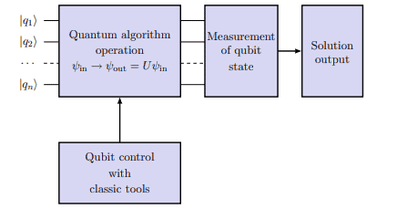
An important step of quantum algorithms is the procedure of measurement of a state. When the qubit state is measured, it randomly passes to one of its states: $|0\rangle$ or $|1\rangle$. Therefore, the complex coefficients $u$ and $v$ from the qubit definition (1.1) are associated with the probability to get the value 0 or 1 when its state is measured. According to the postulates of quantum theory, the probabilities of passing to the states $|0\rangle$ and $|1\rangle$ are equal to $|u|^{2}$ and $|v|^{2}$, respectively. In this connection, the equality (1.2) reflects the probability conservation law. After the measurement, the qubit passes to the basis state, complying with the classical result of the measurement. Generally speaking, the probabilities of getting the result 0 and 1 are different for different states of the quantum system.

In other words, quantum computing is a sequence of simple form operations with the collection of the interacting qubits. In the final step of the quantum computing procedure, the state of the quantum system is measured and a conclusion about the computing result is made. The measurement makes it possible to obtain, at a macroscopic level, the information about the quantum state. The peculiarity of the quantum measurements is their irreversibility, which radically differentiates quantum computing from the classical one.

Despite the fact that the number of qubit states is infinite, with the help of measurement it is possible to obtain only one bit of classical information. The measurement procedure transfers the qubit state to one of the basis states, so a second measurement will produce the same result.

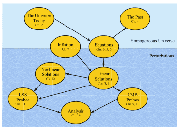
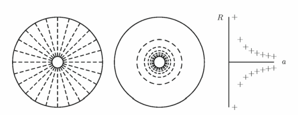
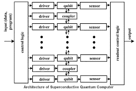
Quantum computer is a set of $n$ qubits controlled by external (classic) signals [812]. Often, an ordered set of some qubits is called a register. The main elements of a quantum computer are shown in Fig. 1.1.

The classical quantum computer setting consists of the controlling classical computer and impulse generators controlling the qubit evolution, as well as measurement instruments of the qubit state. The system from $n$ qubits in the initial state, e.g. $\left|\psi_{\text {in }}\right\rangle=|00 \ldots 0\rangle$, forms a memory register prepared to record input data and perform computations. The data are recorded by an external action on each of the system’s qubits. The solution of the problem is determined by a measurement of the final state qubits $\left|\psi_{\text {out }}\right\rangle[2,12]$.

物理代写|量子计算代写Quantum computer代考|Main elements of a quantum computer

In this record, the state $|\psi\rangle$ of the $n$-qubit register of a quantum computer is expressed through the superposition of vectors of computational basis $B={|0\rangle,|1\rangle, \ldots$, $\left.\left|2^{n}-1\right\rangle\right}$ by the formula
$$
|\psi\rangle=\sum_{k=0}^{2^{n}-1} c_{k}|k\rangle
$$
where the normalization condition
$$
\sum_{k=0}^{2^{k}-1}\left|c_{k}\right|^{2}=1
$$
is met.
A quantum system, formed by $N$ two-level elements, has $\Sigma(N)=2^{N}$ independent states. The key point of the functioning of such a system is the interaction of separate qubits with each other. The number of states $\Sigma(N)$ grows exponentially with the growth of the quantum system, which allows solving practical problems of a very high asymptotic complexity. For example, an efficient quantum algorithm of prime factorization is known, which is very important for cryptography [13]. As a result, the quantum algorithms provide exponential or polynomial speedup in comparison with the classical solution methods for many problems.

Unfortunately, no full-function quantum computer has been created yet, although many of its elements have already been built and studied at the world’s leading laboratories $[11,14,15]$. The main obstacle to the development of quantum computing is the instability of a system of many qubits. The more the qubits are united into an entangled system, the more the effort is required to ensure the smallness of the number of measurement errors. Nevertheless, the history of quantum computer development demonstrates an enormous potential laid in the uniting of quantum theory and algorithm theory.

物理代写|量子计算代写Quantum computer代考|Physics 421

量子计算代考

物理代写|量子计算代写Quantum computer代考|Quantum Computing Model

量子计算机使用具有原子、分子、分子簇等的量子性质的过程。对这些过程的描述是基于复数和复矩阵的应用。

众所周知,经典信息论的基本概念有点[1]。经典位采用值 0 或 1(没有其他值)。

qubit(量子位)是量子计算机中执行信息存储功能的最小元素[2]。

Qubit是一个量子系统|ψ⟩允许两种状态:|0⟩和|1⟩. 根据所谓的“bra-ket”狄拉克“符号(来自单词 bra(c)ket),符号∣0) 和|1⟩读作“凯0“和“Ket 1”,分别。括号|..⟩⟩显示ψ是量子系统的某种状态。

经典比特和量子比特之间的根本区别在于,量子比特可以处于不同于|0⟩或者|1⟩. 量子比特的任意状态由基态的线性组合定义:

|ψ⟩=在|0⟩+在|1⟩,
其中复系数在和在满足以下归一化条件:

|在|2+|在|2=1.
基态的数学描述简化为矩阵形式的表示:

|0⟩=[1 0],|1⟩=[0 1]
根据介绍(1.3),量子位的任意状态写为

|ψ⟩=[在 在]

物理代写|量子计算代写Quantum computer代考|The orthogonality condition

两个状态的正交性条件|ψ′⟩和|ψ′′⟩写成如下:

⟨ψ′∣ψ′′⟩=∑一世=12n在一世∗在一世=0.
请注意,计算基 (1.6) 的状态是正交归一化的。
为了改变量子系统的状态,使用了量子操作,称为量子逻辑门,或者简称为门。因此,门对量子位执行逻辑运算。注意状态的变化|ψ⟩在时间上也被称为量子系统的演化。

量子算法的一个重要步骤是测量状态的过程。当测量量子比特状态时,它会随机进入其状态之一:|0⟩或者|1⟩. 因此,复系数在和在从量子比特定义 (1.1) 中,当测量其状态时,它与获得值 0 或 1 的概率相关联。根据量子理论的假设,传递到状态的概率|0⟩和|1⟩等于|在|2和|在|2, 分别。在这方面,等式(1.2)反映了概率守恒定律。测量后,量子比特进入基态,符合经典的测量结果。一般来说,对于量子系统的不同状态,得到结果 0 和 1 的概率是不同的。

换句话说,量子计算是一系列简单形式的操作,其中包含相互作用的量子比特的集合。在量子计算过程的最后一步,测量量子系统的状态并得出计算结果的结论。测量可以在宏观水平上获得有关量子态的信息。量子测量的特点是它们的不可逆性,这从根本上将量子计算与经典计算区分开来。

尽管量子比特状态的数量是无限的,但在测量的帮助下,可能只获得一位经典信息。测量过程将量子位状态转移到一个基本状态,因此第二次测量将产生相同的结果。

量子计算机是一组n由外部(经典)信号控制的量子比特[812]。通常,一组有序的一些量子比特称为寄存器。量子计算机的主要元件如图 1.1 所示。

经典量子计算机设置包括控制经典计算机和控制量子比特演化的脉冲发生器,以及量子比特状态的测量仪器。该系统从n初始状态的量子比特,例如|ψ在 ⟩=|00…0⟩,形成一个准备记录输入数据和执行计算的内存寄存器。数据是通过对系统的每个量子位进行外部操作来记录的。问题的解决方案由最终状态量子比特的测量决定|ψ出去 ⟩[2,12].

物理代写|量子计算代写Quantum computer代考|Main elements of a quantum computer

在该记录中,该州|ψ⟩的n-量子计算机的qubit寄存器通过计算基向量的叠加来表示B={|0\rangle,|1\rangle, \ldots$, $\left.\left|2^{n}-1\right\rangle\right}B={|0\rangle,|1\rangle, \ldots$, $\left.\left|2^{n}-1\right\rangle\right}由公式

|ψ⟩=∑ķ=02n−1Cķ|ķ⟩
其中归一化条件

∑ķ=02ķ−1|Cķ|2=1
满足。
一个量子系统,由ñ两级元素,有Σ(ñ)=2ñ独立国家。这种系统运行的关键是不同量子位之间的相互作用。状态数Σ(ñ)随着量子系统的增长呈指数增长,这允许解决具有非常高渐近复杂度的实际问题。例如,已知一种有效的素因数分解量子算法,这对密码学非常重要[13]。因此,与许多问题的经典求解方法相比,量子算法提供了指数或多项式加速。

不幸的是,尚未创建全功能的量子计算机,尽管它的许多元素已经在世界领先的实验室建造和研究[11,14,15]. 量子计算发展的主要障碍是多量子比特系统的不稳定性。量子比特越多地结合成一个纠缠系统,就越需要努力确保测量误差的数量很小。尽管如此,量子计算机发展的历史证明了量子理论和算法理论结合的巨大潜力。

物理代写|量子计算代写Quantum computer代考| 请认准statistics-lab™

统计代写请认准statistics-lab™. statistics-lab™为您的留学生涯保驾护航。

金融工程代写

金融工程是使用数学技术来解决金融问题。金融工程使用计算机科学、统计学、经济学和应用数学领域的工具和知识来解决当前的金融问题,以及设计新的和创新的金融产品。

非参数统计代写

非参数统计指的是一种统计方法,其中不假设数据来自于由少数参数决定的规定模型;这种模型的例子包括正态分布模型和线性回归模型。

广义线性模型代考

广义线性模型(GLM)归属统计学领域,是一种应用灵活的线性回归模型。该模型允许因变量的偏差分布有除了正态分布之外的其它分布。

术语 广义线性模型(GLM)通常是指给定连续和/或分类预测因素的连续响应变量的常规线性回归模型。它包括多元线性回归,以及方差分析和方差分析(仅含固定效应)。

有限元方法代写

有限元方法(FEM)是一种流行的方法,用于数值解决工程和数学建模中出现的微分方程。典型的问题领域包括结构分析、传热、流体流动、质量运输和电磁势等传统领域。

有限元是一种通用的数值方法,用于解决两个或三个空间变量的偏微分方程(即一些边界值问题)。为了解决一个问题,有限元将一个大系统细分为更小、更简单的部分,称为有限元。这是通过在空间维度上的特定空间离散化来实现的,它是通过构建对象的网格来实现的:用于求解的数值域,它有有限数量的点。边界值问题的有限元方法表述最终导致一个代数方程组。该方法在域上对未知函数进行逼近。[1] 然后将模拟这些有限元的简单方程组合成一个更大的方程系统,以模拟整个问题。然后,有限元通过变化微积分使相关的误差函数最小化来逼近一个解决方案。

tatistics-lab作为专业的留学生服务机构,多年来已为美国、英国、加拿大、澳洲等留学热门地的学生提供专业的学术服务,包括但不限于Essay代写,Assignment代写,Dissertation代写,Report代写,小组作业代写,Proposal代写,Paper代写,Presentation代写,计算机作业代写,论文修改和润色,网课代做,exam代考等等。写作范围涵盖高中,本科,研究生等海外留学全阶段,辐射金融,经济学,会计学,审计学,管理学等全球99%专业科目。写作团队既有专业英语母语作者,也有海外名校硕博留学生,每位写作老师都拥有过硬的语言能力,专业的学科背景和学术写作经验。我们承诺100%原创,100%专业,100%准时,100%满意。

随机分析代写


随机微积分是数学的一个分支,对随机过程进行操作。它允许为随机过程的积分定义一个关于随机过程的一致的积分理论。这个领域是由日本数学家伊藤清在第二次世界大战期间创建并开始的。

时间序列分析代写

随机过程,是依赖于参数的一组随机变量的全体,参数通常是时间。 随机变量是随机现象的数量表现,其时间序列是一组按照时间发生先后顺序进行排列的数据点序列。通常一组时间序列的时间间隔为一恒定值(如1秒,5分钟,12小时,7天,1年),因此时间序列可以作为离散时间数据进行分析处理。研究时间序列数据的意义在于现实中,往往需要研究某个事物其随时间发展变化的规律。这就需要通过研究该事物过去发展的历史记录,以得到其自身发展的规律。

回归分析代写

多元回归分析渐进(Multiple Regression Analysis Asymptotics)属于计量经济学领域,主要是一种数学上的统计分析方法,可以分析复杂情况下各影响因素的数学关系,在自然科学、社会和经济学等多个领域内应用广泛。

MATLAB代写

MATLAB 是一种用于技术计算的高性能语言。它将计算、可视化和编程集成在一个易于使用的环境中,其中问题和解决方案以熟悉的数学符号表示。典型用途包括:数学和计算算法开发建模、仿真和原型制作数据分析、探索和可视化科学和工程图形应用程序开发,包括图形用户界面构建MATLAB 是一个交互式系统,其基本数据元素是一个不需要维度的数组。这使您可以解决许多技术计算问题,尤其是那些具有矩阵和向量公式的问题,而只需用 C 或 Fortran 等标量非交互式语言编写程序所需的时间的一小部分。MATLAB 名称代表矩阵实验室。MATLAB 最初的编写目的是提供对由 LINPACK 和 EISPACK 项目开发的矩阵软件的轻松访问,这两个项目共同代表了矩阵计算软件的最新技术。MATLAB 经过多年的发展,得到了许多用户的投入。在大学环境中,它是数学、工程和科学入门和高级课程的标准教学工具。在工业领域,MATLAB 是高效研究、开发和分析的首选工具。MATLAB 具有一系列称为工具箱的特定于应用程序的解决方案。对于大多数 MATLAB 用户来说非常重要,工具箱允许您学习应用专业技术。工具箱是 MATLAB 函数(M 文件)的综合集合,可扩展 MATLAB 环境以解决特定类别的问题。可用工具箱的领域包括信号处理、控制系统、神经网络、模糊逻辑、小波、仿真等。

R语言代写问卷设计与分析代写
PYTHON代写回归分析与线性模型代写
MATLAB代写方差分析与试验设计代写
STATA代写机器学习/统计学习代写
SPSS代写计量经济学代写
EVIEWS代写时间序列分析代写
EXCEL代写深度学习代写
SQL代写各种数据建模与可视化代写

物理代写|宇宙学代写cosmology代考|PHYS 3080

如果你也在 怎样代写宇宙学cosmology这个学科遇到相关的难题,请随时右上角联系我们的24/7代写客服。

宇宙学是天文学的一个分支,涉及宇宙的起源和演变,从大爆炸到今天,再到未来。宇宙学的定义是 “对整个宇宙的大尺度特性进行科学研究”。

statistics-lab™ 为您的留学生涯保驾护航 在代写宇宙学cosmology方面已经树立了自己的口碑, 保证靠谱, 高质且原创的统计Statistics代写服务。我们的专家在代写宇宙学cosmology代写方面经验极为丰富,各种代写宇宙学cosmology相关的作业也就用不着说。

我们提供的宇宙学cosmology及其相关学科的代写,服务范围广, 其中包括但不限于:

  • Statistical Inference 统计推断
  • Statistical Computing 统计计算
  • Advanced Probability Theory 高等概率论
  • Advanced Mathematical Statistics 高等数理统计学
  • (Generalized) Linear Models 广义线性模型
  • Statistical Machine Learning 统计机器学习
  • Longitudinal Data Analysis 纵向数据分析
  • Foundations of Data Science 数据科学基础
物理代写|宇宙学代写cosmology代考|PHYS 3080

物理代写|宇宙学代写cosmology代考|Standard Model of particle physics

The Standard Model of particle physics describes the known fundamental particles in nature and how they interact. The particles can be divided into two classes: spin-1/2 fermions and integer-spin bosons.

Fermions are the constituents of matter: the quarks, out of which baryons are built, and the leptons such as electrons and neutrinos. There are three generations with two quarks each for a total of six quarks, denoted $u, d ; s, c ; b, t$. Each generation of quarks is associated with a pair of leptons. For example, the $u, d$ pair is associated with the electron and its neutrino: $e^{-}, v_{e}$. The other lepton pairs are $\mu^{-}, v_{\mu}$ and $\tau^{-}, v_{\tau}$. The vast majority of matter in the universe is made up of the first generation, with the exception of neutrinos, which are mixed between the different generations. Unlike leptons, quarks do not exist on their own, but they form bound states under the strong interaction. Baryons, the most important ones being the proton and neutron, are made out of three quarks. Mesons are composed of a quark-antiquark pair.

Bosons contain the spin-1 (vector) force carriers, the most famous of which is the photon which mediates the electromagnetic force. There are eight gluons (massless, like the photon) that mediate the strong force. The weak force, responsible for example for neutron decay, is mediated by three massive bosons: the $Z, W^{+}$and $W^{-}$. These force mediators are complemented with the spin-0 (scalar) Higgs boson. The Higgs couples to all massive fermions as well as the $W$ and $Z$ bosons. This coupling gives mass to the particles through the Higgs’ homogeneous background field value.

The Standard Model has remained largely intact since its inception, gaining more and more experimental verification every year. However, neutrino masses are now a confirmed piece of physics beyond the Standard Model. Moreover, the evidence cosmologists have uncovered-that there is a need for dark matter, dark energy, and new physics leading to inflation-clearly shows that the Standard Model is not the final word in particle physics.

物理代写|宇宙学代写cosmology代考|the concordance model of cosmology

We are now ready to summarize the concordance model of cosmology: a Euclidean universe that is dominated today by non-baryonic cold dark matter (CDM) and a cosmological constant, with initial perturbations generated by inflation in the very early universe. Since all measurements are currently consistent with dark energy being a cosmological constant $\Lambda$, this concordance model of cosmology has become known as (flat) $\Lambda$ CDM. It is worth noting that none of these ingredients are part of the Standard Model of particle physics (Box 1.1)! Let us thus briefly discuss the status of these three ingredients.

CDM: The “Cold” part of this moniker comes from requiring the dark matter particles to be able to clump efficiently in the early universe. If they are hot instead, i.e., have large velocities, structure will not form at the appropriate levels; among others, this excludes the known neutrinos from being dark matter candidates. We have argued that BBN and the CMB imply the existence of non-baryonic matter. However, observations of structure in the universe independently lead to the conclusion that there must be dark matter. The inhomogeneities expected in a model without dark matter are far too small. In Ch. 8, we will come to understand the reason why a baryon-only universe would be so smooth. Moreover, dark matter is a familiar concept to astronomers; the first suggestion was put forth by Zwicky (1933), based on galaxy velocities within clusters. Ample evidence also comes from the rotation curves of galaxies. Indeed, a mismatch between the matter inferred from gravity and that which we can see in the form of baryons exists on all galactic and extragalactic scales, and it always points toward roughly 5 times more dark matter than baryons.

What is this new form of matter? And how did it form in the early universe? So far, we know only its overall abundance and the fact that it must be cold. The most popular idea currently is that the dark matter consists of elementary particles produced during early moments of the Big Bang. In Ch. 4, we will explore this possibility in detail, arguing that dark matter may have been produced when the temperature of the universe was of order hundreds of $\mathrm{GeV} / k_{\mathrm{B}}$. As we will see, the hypothesis that dark matter consists of fundamental relics from the early universe is being rigorously tested experimentally.

Cosmological constant: Evidence from a variety of sources, but most famously from distant supernovae (starting with Riess et al., 1998; Perlmutter et al., 1999) suggests that there must be energy, dark energy, besides ordinary matter and radiation. Unlike dark matter, this component does not cluster strongly. We already discussed the possibility that this new form of energy remains constant with time, i.e., acts as a cosmological constant, a possibility first introduced (and later abandoned) by Einstein. Cosmologists have explored other forms though, many of which behave quite differently from the cosmological constant. We will see more of this in Sect. 2.4.6.

物理代写|宇宙学代写cosmology代考|Summary and outlook

As a way of summarizing the features of an expanding universe that we have outlined above and that we will explore in great detail in the coming chapters, let us construct a time line. We can equivalently characterize any epoch in the universe by the time since the Big Bang; by the value of the scale factor at that time; by the redshift freely traveling photons have experienced from then until today or by the temperature of the cosmic background radiation. For example, today, $t \simeq 13.7$ billion years; $a=1 ; z=0$; and $T=2.73 \mathrm{~K}=2.35 \times 10^{-4} \mathrm{eV} / k_{B}$. Fig. $1.11$ shows a time line of the universe using both time and temperature as markers. The milestones indicated on the time line range from those that involve known physics (nucleosynthesis and the CMB) to those that go beyond the Standard Model of particle physics (inflation and dark energy).

The time line in Fig. $1.11$ shows the dominant component of the universe at various times. We do not know what dominated the energy budget of the universe at very early times after the end of inflation. We do know, however, that the universe was dominated by radiation at the latest by the time BBN occurred. Eventually, since the energy of a relativistic particle falls as $1 / a$ while that of a nonrelativistic particle remains constant at $m$, matter overtook radiation. At relatively recent times, the universe has become dominated not by matter, but by dark energy, whose density remains approximately constant with time.
The classical results in cosmology can be understood in the context of a smooth universe. Light elements formed when the universe was several minutes old, and the CMB decoupled from matter at a temperature of order $k_{\mathrm{B}} T \sim 1 / 4 \mathrm{eV}$, when the universe was 380,000 years old. Heavy elementary particles may make up the dark matter in the universe; if they do, their abundance was fixed at very high temperatures of order $k_{\mathrm{B}} T \sim$ $100 \mathrm{GeV}$ or higher.

In this book, we will be mostly interested in the perturbations around the smooth universe. At the beginning of the time line, we allow for a brief period of inflation, during which primordial perturbations were produced. These small perturbations began to grow when the universe became dominated by matter. The dark matter grew more and more clumpy, simply because of the attractive nature of gravity. An overdensity of dark matter of 1 part in 1000 when the temperature was $1 \mathrm{eV}$ grew to 1 part in 100 by the time the temperature dropped to $0.1 \mathrm{eV}$. Eventually, at relatively recent times, perturbations in the matter ceased to be small; they became the nonlinear structure we see today. The observed anisotropies in the CMB tell us what the universe looked like when perturbations were very small, so they are a wonderful probe of the latter. Moreover, the CMB anisotropies provide a precise characterization of the initial conditions needed for detailed analytic and numerical studies of the growth of structure. To give you an idea of the road ahead, Fig. $1.12$ charts the way through the various ingredients going into this calculation that we will get to know in subsequent chapters of the book.

Some of the elements in the time line we have discussed may well be incorrect. However, since most of these ideas are testable, the data from the first half of the 21st century will tell us which parts of the time line are correct and which need to be discarded. This in itself seems more than sufficient reason to study the CMB and large-scale structure.

物理代写|宇宙学代写cosmology代考|PHYS 3080

宇宙学代考

物理代写|宇宙学代写cosmology代考|Standard Model of particle physics

粒子物理学的标准模型描述了自然界中已知的基本粒子以及它们如何相互作用。粒子可以分为两类:自旋1/2费米子和整数自旋玻色子。

费米子是物质的组成部分:构成重子的夸克,以及电子和中微子等轻子。有 3 代,每代有 2 个夸克,总共有 6 个夸克,记为在,d;s,C;b,吨. 每一代夸克都与一对轻子有关。例如,在,dpair 与电子及其中微子有关:和−,在和. 其他轻子对是μ−,在μ和τ−,在τ. 宇宙中的绝大多数物质都是由第一代组成的,除了中微子,它们在不同代之间混合。与轻子不同的是,夸克本身并不存在,而是在强相互作用下形成束缚态。重子,最重要的是质子和中子,由三个夸克组成。介子由夸克-反夸克对组成。

玻色子包含自旋 1(矢量)力载体,其中最著名的是介导电磁力的光子。有 8 个胶子(无质量,如光子)调节强力。导致中子衰变的弱力是由三个大质量玻色子介导的:从,在+和在−. 这些力介质与自旋 0(标量)希格斯玻色子相辅相成。希格斯对所有大质量费米子以及在和从玻色子。这种耦合通过希格斯的均匀背景场值为粒子提供质量。

标准模型自成立以来基本保持不变,每年都获得越来越多的实验验证。然而,中微子质量现在是超出标准模型的已证实的物理学部分。此外,宇宙学家发现的证据——需要暗物质、暗能量和导致暴胀的新物理学——清楚地表明,标准模型并不是粒子物理学的最终定论。

物理代写|宇宙学代写cosmology代考|the concordance model of cosmology

我们现在准备总结宇宙学的一致性模型:今天由非重子冷暗物质 (CDM) 和宇宙学常数主导的欧几里得宇宙,初始扰动由早期宇宙中的膨胀产生。由于目前所有测量结果都与暗能量是宇宙学常数一致Λ,这个宇宙学的一致性模型被称为(平面)Λ清洁发展机制。值得注意的是,这些成分都不是粒子物理标准模型的一部分(框 1.1)!因此,让我们简要讨论这三种成分的状态。

CDM:这个绰号的“冷”部分来自于要求暗物质粒子能够在早期宇宙中有效地聚集。如果它们是热的,即速度很大,则不会在适当的水平上形成结构;除其他外,这将已知的中微子排除在暗物质候选者之外。我们认为 BBN 和 CMB 暗示了非重子物质的存在。然而,对宇宙结构的观察独立地得出结论,即一定存在暗物质。在没有暗物质的模型中预期的不均匀性太小了。英寸。8,我们将理解为什么只有重子的宇宙会如此平滑。此外,暗物质是天文学家熟悉的概念。第一个建议是 Zwicky (1933) 基于星系团内的星系速度提出的。充足的证据还来自星系的自转曲线。事实上,从引力推断出的物质与我们以重子形式看到的物质之间存在不匹配,存在于所有银河系和银河系外的尺度上,它总是指向比重子多约 5 倍的暗物质。

这种新形式的物质是什么?它是如何在早期宇宙中形成的?到目前为止,我们只知道它的总体丰度以及它一定很冷的事实。目前最流行的想法是暗物质由大爆炸早期产生的基本粒子组成。英寸。4,我们将详细探讨这种可能性,认为暗物质可能是在宇宙温度达到数百摄氏度时产生的G和在/ķ乙. 正如我们将看到的,暗物质由早期宇宙的基本遗迹组成的假设正在经过严格的实验检验。

宇宙常数:来自各种来源的证据,但最著名的是来自遥远的超新星(从 Riess 等人,1998 年;Perlmutter 等人,1999 年开始)表明除了普通物质和辐射之外,还必须有能量、暗能量。与暗物质不同,该成分不会强烈聚集。我们已经讨论过这种新形式的能量随时间保持不变的可能性,即作为宇宙常数,这是爱因斯坦首先引入(后来放弃)的可能性。不过,宇宙学家已经探索了其他形式,其中许多的行为与宇宙学常数完全不同。我们将在 Sect 中看到更多这样的内容。2.4.6。

物理代写|宇宙学代写cosmology代考|Summary and outlook

作为总结我们上面概述的膨胀宇宙特征的一种方式,我们将在接下来的章节中详细探讨,让我们构建一个时间线。我们可以等价地描述宇宙大爆炸以来的任何时代;由当时的比例因子的值;从那时到今天,自由行进的光子经历了红移,或者宇宙背景辐射的温度。例如,今天,吨≃13.7亿年;一个=1;和=0; 和吨=2.73 ķ=2.35×10⁻⁴和在/ķ乙. 如图。1.11使用时间和温度作为标记显示了宇宙的时间线。时间线上显示的里程碑范围从涉及已知物理学(核合成和 CMB)到超出粒子物理学标准模型(膨胀和暗能量)的里程碑。

时间线如图。1.11显示了不同时期宇宙的主要组成部分。我们不知道在暴胀结束后的早期,是什么主导了宇宙的能量收支。然而,我们确实知道,最迟在 BBN 发生时,宇宙已被辐射支配。最终,由于相对论粒子的能量下降为1/一个而非相对论粒子的粒子保持不变米,物质超过了辐射。在最近的一段时间里,宇宙不再由物质主导,而是由暗能量主导,其密度随时间保持大致恒定。
宇宙学的经典结果可以在平滑宇宙的背景下理解。轻元素在宇宙诞生几分钟时形成,而 CMB 在一定温度下与物质分离ķ乙吨∼1/4和在,当宇宙有 38 万年的历史时。重基本粒子可能构成宇宙中的暗物质;如果他们这样做了,他们的丰度就被固定在非常高的秩序温度下ķ乙吨∼ 100G和在或更高。

在本书中,我们最感兴趣的是围绕平滑宇宙的扰动。在时间线的开始,我们允许短暂的暴胀时期,在此期间会产生原始扰动。当宇宙被物质支配时,这些微小的扰动开始增长。暗物质变得越来越块状,仅仅是因为引力的吸引力。温度为 1000 分之一的暗物质超密度1和在到温度下降到 100 分之一0.1和在. 最终,在最近的一段时间里,对此事的扰动不再很小。它们变成了我们今天看到的非线性结构。在 CMB 中观察到的各向异性告诉我们,当扰动非常小时,宇宙是什么样子的,因此它们是对后者的一个很好的探索。此外,CMB 各向异性提供了对结构生长的详细分析和数值研究所需的初始条件的精确表征。为了让您了解未来的道路,图。1.12图表显示了计算中的各种成分,我们将在本书的后续章节中了解这些成分。

我们讨论过的时间线中的一些元素很可能是不正确的。然而,由于这些想法大部分都是可以检验的,21世纪上半叶的数据会告诉我们时间线的哪些部分是正确的,哪些需要丢弃。这本身似乎是研究 CMB 和大型结构的充分理由。

物理代写|宇宙学代写cosmology代考 请认准statistics-lab™

统计代写请认准statistics-lab™. statistics-lab™为您的留学生涯保驾护航。

金融工程代写

金融工程是使用数学技术来解决金融问题。金融工程使用计算机科学、统计学、经济学和应用数学领域的工具和知识来解决当前的金融问题,以及设计新的和创新的金融产品。

非参数统计代写

非参数统计指的是一种统计方法,其中不假设数据来自于由少数参数决定的规定模型;这种模型的例子包括正态分布模型和线性回归模型。

广义线性模型代考

广义线性模型(GLM)归属统计学领域,是一种应用灵活的线性回归模型。该模型允许因变量的偏差分布有除了正态分布之外的其它分布。

术语 广义线性模型(GLM)通常是指给定连续和/或分类预测因素的连续响应变量的常规线性回归模型。它包括多元线性回归,以及方差分析和方差分析(仅含固定效应)。

有限元方法代写

有限元方法(FEM)是一种流行的方法,用于数值解决工程和数学建模中出现的微分方程。典型的问题领域包括结构分析、传热、流体流动、质量运输和电磁势等传统领域。

有限元是一种通用的数值方法,用于解决两个或三个空间变量的偏微分方程(即一些边界值问题)。为了解决一个问题,有限元将一个大系统细分为更小、更简单的部分,称为有限元。这是通过在空间维度上的特定空间离散化来实现的,它是通过构建对象的网格来实现的:用于求解的数值域,它有有限数量的点。边界值问题的有限元方法表述最终导致一个代数方程组。该方法在域上对未知函数进行逼近。[1] 然后将模拟这些有限元的简单方程组合成一个更大的方程系统,以模拟整个问题。然后,有限元通过变化微积分使相关的误差函数最小化来逼近一个解决方案。

tatistics-lab作为专业的留学生服务机构,多年来已为美国、英国、加拿大、澳洲等留学热门地的学生提供专业的学术服务,包括但不限于Essay代写,Assignment代写,Dissertation代写,Report代写,小组作业代写,Proposal代写,Paper代写,Presentation代写,计算机作业代写,论文修改和润色,网课代做,exam代考等等。写作范围涵盖高中,本科,研究生等海外留学全阶段,辐射金融,经济学,会计学,审计学,管理学等全球99%专业科目。写作团队既有专业英语母语作者,也有海外名校硕博留学生,每位写作老师都拥有过硬的语言能力,专业的学科背景和学术写作经验。我们承诺100%原创,100%专业,100%准时,100%满意。

随机分析代写


随机微积分是数学的一个分支,对随机过程进行操作。它允许为随机过程的积分定义一个关于随机过程的一致的积分理论。这个领域是由日本数学家伊藤清在第二次世界大战期间创建并开始的。

时间序列分析代写

随机过程,是依赖于参数的一组随机变量的全体,参数通常是时间。 随机变量是随机现象的数量表现,其时间序列是一组按照时间发生先后顺序进行排列的数据点序列。通常一组时间序列的时间间隔为一恒定值(如1秒,5分钟,12小时,7天,1年),因此时间序列可以作为离散时间数据进行分析处理。研究时间序列数据的意义在于现实中,往往需要研究某个事物其随时间发展变化的规律。这就需要通过研究该事物过去发展的历史记录,以得到其自身发展的规律。

回归分析代写

多元回归分析渐进(Multiple Regression Analysis Asymptotics)属于计量经济学领域,主要是一种数学上的统计分析方法,可以分析复杂情况下各影响因素的数学关系,在自然科学、社会和经济学等多个领域内应用广泛。

MATLAB代写

MATLAB 是一种用于技术计算的高性能语言。它将计算、可视化和编程集成在一个易于使用的环境中,其中问题和解决方案以熟悉的数学符号表示。典型用途包括:数学和计算算法开发建模、仿真和原型制作数据分析、探索和可视化科学和工程图形应用程序开发,包括图形用户界面构建MATLAB 是一个交互式系统,其基本数据元素是一个不需要维度的数组。这使您可以解决许多技术计算问题,尤其是那些具有矩阵和向量公式的问题,而只需用 C 或 Fortran 等标量非交互式语言编写程序所需的时间的一小部分。MATLAB 名称代表矩阵实验室。MATLAB 最初的编写目的是提供对由 LINPACK 和 EISPACK 项目开发的矩阵软件的轻松访问,这两个项目共同代表了矩阵计算软件的最新技术。MATLAB 经过多年的发展,得到了许多用户的投入。在大学环境中,它是数学、工程和科学入门和高级课程的标准教学工具。在工业领域,MATLAB 是高效研究、开发和分析的首选工具。MATLAB 具有一系列称为工具箱的特定于应用程序的解决方案。对于大多数 MATLAB 用户来说非常重要,工具箱允许您学习应用专业技术。工具箱是 MATLAB 函数(M 文件)的综合集合,可扩展 MATLAB 环境以解决特定类别的问题。可用工具箱的领域包括信号处理、控制系统、神经网络、模糊逻辑、小波、仿真等。

R语言代写问卷设计与分析代写
PYTHON代写回归分析与线性模型代写
MATLAB代写方差分析与试验设计代写
STATA代写机器学习/统计学习代写
SPSS代写计量经济学代写
EVIEWS代写时间序列分析代写
EXCEL代写深度学习代写
SQL代写各种数据建模与可视化代写

物理代写|宇宙学代写cosmology代考|PHYSICS 1002

如果你也在 怎样代写宇宙学cosmology这个学科遇到相关的难题,请随时右上角联系我们的24/7代写客服。

宇宙学是天文学的一个分支,涉及宇宙的起源和演变,从大爆炸到今天,再到未来。宇宙学的定义是 “对整个宇宙的大尺度特性进行科学研究”。

statistics-lab™ 为您的留学生涯保驾护航 在代写宇宙学cosmology方面已经树立了自己的口碑, 保证靠谱, 高质且原创的统计Statistics代写服务。我们的专家在代写宇宙学cosmology代写方面经验极为丰富,各种代写宇宙学cosmology相关的作业也就用不着说。

我们提供的宇宙学cosmology及其相关学科的代写,服务范围广, 其中包括但不限于:

  • Statistical Inference 统计推断
  • Statistical Computing 统计计算
  • Advanced Probability Theory 高等概率论
  • Advanced Mathematical Statistics 高等数理统计学
  • (Generalized) Linear Models 广义线性模型
  • Statistical Machine Learning 统计机器学习
  • Longitudinal Data Analysis 纵向数据分析
  • Foundations of Data Science 数据科学基础
物理代写|宇宙学代写cosmology代考|PHYSICS 1002

物理代写|宇宙学代写cosmology代考|Big Bang nucleosynthesis

Armed with an understanding of the evolution of the scale factor and the densities of the constituents in the universe, we can extrapolate backwards to explore phenomena at early times. When the universe was much hotter and denser, and the temperature was of order $1 \mathrm{MeV} / k_{\mathrm{B}}$, there were no neutral atoms or even bound nuclei. The vast amounts of highenergy radiation in such a hot environment ensured that any atom or nucleus produced would be immediately destroyed by a high-energy photon. As the universe cooled well below typical nuclear binding energies, light elements began to form in a process known as Big Bang Nucleosynthesis (BBN). Knowing the conditions of the early universe and the relevant nuclear cross-sections, we can calculate the expected primordial abundances of all the elements (Ch. 4).

Fig. $1.6$ shows the BBN predictions for the abundances of helium and deuterium as a function of the mean baryon density, essentially the density of ordinary matter (Sect. $2.4$ ) in the universe, in units of the critical density. The predicted abundances, in particular that of deuterium, which we will explore in detail in Ch. 4, depend on the density of protons and neutrons at the time of nucleosynthesis. The combined proton plus neutron density is equal to the baryon density since both protons and neutrons have baryon number one and these are the only baryons around at the time.

The horizontal lines in Fig. 1.6 show the current measurements of the light element abundances. The deuterium abundance is measured in the intergalactic medium at high redshifts by looking for a subtle absorption feature in the spectrum of distant quasars (see Burles and Tytler, 1998; Cooke et al., 2018 and Exercise 1.3). These measurements of the abundances, combined with BBN calculations, give us a way of measuring the baryon density in the universe, constraining ordinary matter to contribute at most $5 \%$ of the critical density (note that the $x$-axis in Fig. $1.6$ is the baryon density divided by the critical density, but multiplied by $h^{2} \simeq 0.5$ ). Since the total matter density today is significantly larger than this-as we will see throughout the book-nucleosynthesis provides a compelling argument for matter that is comprised of neither protons or neutrons. This new type of matter has been dubbed dark matter because it apparently does not emit light. One of the central questions in physics now is: “What is the Dark Matter?”

物理代写|宇宙学代写cosmology代考|The cosmic microwave background

Another phenomenon that falls out of energetics and a qualitative understanding of the evolution of the universe is the origin of the CMB. When the temperature of the radiation was of order $10^{4} \mathrm{~K}$ (corresponding to energies of order an $\mathrm{eV}$ ), free electrons and protons combined to form neutral hydrogen. Before then, any hydrogen produced was quickly ionized by energetic photons. After that epoch, at $z \simeq 1100$, the photons that comprise the CMB ceased interacting with any particles and traveled freely through space. When we observe them today, we are thus looking at messengers from an early moment in the universe’s history. They are therefore the most powerful probes of the early universe. We will spend an inordinate amount of time in this book working through the details of what happened to the photons before they last scattered off of free electrons, and also developing the mathematics of the free-streaming process since then. Among many other aspects, we will understand how the CMB constrains the baryon density independently, and in agreement with BBN as shown in Fig. 1.6, providing a ringing confirmation of the concordance model.

For now, we are only concerned with the crucial fact that the interactions of photons with electrons before last scattering ensured that the photons were in equilibrium. That is, they should have a black-body spectrum. The specific intensity of a gas of photons with a black-body spectrum is
$$
I_{v}=\frac{4 \pi \hbar v^{3} / c^{2}}{\exp \left[2 \pi \hbar v / k_{\mathrm{B}} T\right]-1} .
$$
Fig. 1.7 shows the remarkable agreement between this prediction (see Exercise 1.4) of Big Bang cosmology and the observations by the FIRAS instrument aboard the COBE satellite. In fact, the CMB provides the best black-body spectrum ever measured. We have been told ${ }^{2}$ that detection of the $3 \mathrm{~K}$ background by Penzias and Wilson in the mid-1960s was sufficient evidence to decide the controversy in favor of the Big Bang over the Steady State universe, an alternative scenario without any expansion. Penzias and Wilson, though, measured the radiation at just one wavelength. If even their one-wavelength result was enough to tip the scales, the current data depicted in Fig. $1.7$ should send skeptics from the pages of physics journals to the far reaches of radical internet chat groups.

物理代写|宇宙学代写cosmology代考|Structure in the universe

The existence of structure in the universe was known long before the detection of CMB anisotropies: various efforts to map out the distribution of galaxies in the local universe clearly showed that they are not distributed homogeneously. The number of galaxies and volume covered by such surveys has grown exponentially. Two surveys in particular broke new ground: the Sloan Digital Sky Survey (SDSS; Fig. 1.8) and the Two Degree Field Galaxy Redshift Survey (2dF), which between them compiled the redshifts of, and hence the distances to, over a million galaxies. Projects over the ensuing decades have and will provide deeper and more detailed maps than these ground-breaking surveys, by orders of magnitude.

The galaxies in Fig. $1.8$ are clearly not distributed randomly: the universe has structure on large scales. To understand this structure, we must develop the tools to study perturbations around the smooth background. We will see that this is straightforward in theory, as long as the perturbations remain small. To compare theory with observations, we must thus try to avoid regimes that cannot be described by small perturbations. As an extreme example, we can never hope to understand cosmology by carefully examining rock formations on Earth. The intermediate steps-collapse of matter into a galaxy; star formation; planet formation; geology; etc.-are much too complicated to allow comparison between linear theory and observations. In fact, perturbations to the matter on small scales (less than about $10 \mathrm{Mpc}$ ) have become large in the late universe; that is, the fractional density fluctuations on these scales are not small, but comparable to or larger than unity. We say that these scales have grown nonlinear. On the other hand, large-scale perturbations are still small (quasi-linear). So they have been processed much less than the small-scale structure. Similarly, anisotropies in the CMB are small because they originated at early times and the photons that we observe from the CMB do not clump on their way to us. Because of this, the best ways to learn about the evolution of structure and to compare theory with observations are to look at anisotropies in the CMB and at large-scale structure (LSS), i.e. how galaxies and matter are distributed on large scales. However, we will learn in Chs. 12-13 that valuable cosmological information can also be extracted from smaller, nonlinear scales provided we choose our observables wisely.

It is paramount therefore to develop statistics that can empower us to compare maps like that shown in Fig. $1.8$ to theories while isolating large scales from small scales. For this purpose, it is often useful to take the Fourier transform of the distribution in question; as we will see, working in Fourier space makes it easier to separate large from small scales. The most important statistic in the cases of both the CMB and the large-scale structure is the two-point function, short-hand for two-point correlation function. When measured using Fourier-space fields, it is called the power spectrum.

物理代写|宇宙学代写cosmology代考|PHYSICS 1002

宇宙学代考

物理代写|宇宙学代写cosmology代考|Big Bang nucleosynthesis

了解了尺度因子的演变和宇宙中成分的密度后,我们可以向后推断以探索早期的现象。当宇宙变得更热更稠密,并且温度有序时1米和在/ķ乙,没有中性原子,甚至没有结合的原子核。在如此炎热的环境中,大量的高能辐射确保产生的任何原子或原子核都会立即被高能光子摧毁。当宇宙冷却到远低于典型的核结合能时,轻元素开始在被称为大爆炸核合成(BBN)的过程中形成。了解早期宇宙的条件和相关的核截面,我们可以计算所有元素的预期原始丰度(第 4 章)。

如图。1.6显示了 BBN 对氦和氘丰度的预测,它是平均重子密度的函数,本质上是普通物质的密度(Sect.2.4) 在宇宙中,以临界密度为单位。预测的丰度,特别是氘的丰度,我们将在第 1 章详细探讨。4、取决于核合成时质子和中子的密度。质子加中子的组合密度等于重子密度,因为质子和中子都有第一号重子,而这些是当时唯一的重子。

图 1.6 中的水平线显示了轻元素丰度的当前测量值。通过寻找遥远类星体光谱中的细微吸收特征,在高红移的星系际介质中测量氘丰度(参见 Burles 和 Tytler,1998;Cooke 等,2018 和练习 1.3)。这些丰度测量,结合 BBN 计算,为我们提供了一种测量宇宙中重子密度的方法,限制普通物质最多贡献5%的临界密度(注意X- 图中的轴1.6是重子密度除以临界密度,但乘以H2≃0.5)。由于今天的总物质密度远大于此——正如我们将在整本书中看到的那样——核合成为既不由质子也不由中子组成的物质提供了令人信服的论据。这种新型物质被称为暗物质,因为它显然不发光。现在物理学的核心问题之一是:“什么是暗物质?”

物理代写|宇宙学代写cosmology代考|The cosmic microwave background

另一个脱离能量学和对宇宙演化定性理解的现象是 CMB 的起源。当辐射温度正常时104 ķ(对应于秩序的能量和在),自由电子和质子结合形成中性氢。在此之前,产生的任何氢都会被高能光子迅速电离。在那个时代之后,在和≃1100,构成 CMB 的光子停止与任何粒子相互作用并在空间中自由行进。当我们今天观察它们时,我们正在观察宇宙历史早期的信使。因此,它们是早期宇宙中最强大的探测器。我们将在本书中花费大量时间来研究光子在最后一次散射出自由电子之前发生的事情的细节,并从那时起开发自由流过程的数学。在许多其他方面,我们将了解 CMB 如何独立约束重子密度,并与 BBN 一致,如图 1.6 所示,提供一致性模型的振铃确认。

目前,我们只关心最后一次散射之前光子与电子的相互作用确保光子处于平衡状态这一关键事实。也就是说,它们应该具有黑体光谱。具有黑体光谱的光子气体的比强度为

我在=4圆周率ℏ在3/C2经验⁡[2圆周率ℏ在/ķ乙吨]−1.
图 1.7 显示了大爆炸宇宙学的这一预测(见练习 1.4)与 COBE 卫星上的 FIRAS 仪器的观测结果之间的显着一致性。事实上,CMB 提供了有史以来最好的黑体光谱。我们被告知2该检测3 ķ彭齐亚斯和威尔逊在 1960 年代中期的背景足以证明大爆炸对稳态宇宙的争议,这是一种没有任何膨胀的替代方案。然而,彭齐亚斯和威尔逊只测量了一种波长的辐射。如果即使他们的单波长结果也足以使天平倾斜,那么图 1 中描绘的当前数据。1.7应该将怀疑论者从物理期刊的页面发送到激进的互联网聊天组的远端。

物理代写|宇宙学代写cosmology代考|Structure in the universe

早在探测到 CMB 各向异性之前,宇宙中结构的存在就已为人所知:绘制局部宇宙中星系分布的各种努力清楚地表明它们分布不均匀。此类调查所涵盖的星系数量和体积呈指数增长。特别是两项调查开辟了新天地:斯隆数字巡天(SDSS;图 1.8)和两度视场星系红移调查(2dF),它们之间汇总了超过一百万个星系的红移以及与它们之间的距离. 随后几十年的项目已经并将提供比这些开创性调查更深入和更详细的地图,数量级。

图中的星系。1.8显然不是随机分布的:宇宙具有大尺度的结构。为了理解这种结构,我们必须开发工具来研究围绕平滑背景的扰动。我们将看到这在理论上是直截了当的,只要扰动仍然很小。因此,为了将理论与观察结果进行比较,我们必须尽量避免使用小扰动无法描述的状态。作为一个极端的例子,我们永远无法通过仔细检查地球上的岩层来理解宇宙学。中间步骤——物质坍缩成星系;恒星形成;行星形成;地质学; 等等-太复杂了,无法在线性理论和观察之间进行比较。事实上,对小尺度物质的扰动(小于约10米pC) 在宇宙晚期变大了;也就是说,这些尺度上的分数密度波动并不小,而是与统一相当或更大。我们说这些尺度已经变得非线性。另一方面,大尺度扰动仍然很小(准线性)。因此,它们的加工量远低于小型结构。同样,CMB 中的各向异性很小,因为它们起源于早期,而且我们从 CMB 观察到的光子在到达我们的途中不会聚集。正因为如此,了解结构演化以及将理论与观测结果进行比较的最佳方法是观察 CMB 和大尺度结构 (LSS) 中的各向异性,即星系和物质在大尺度上的分布情况。但是,我们将在 Chs 中学习。

因此,开发能够使我们能够比较如图所示的地图的统计数据至关重要。1.8理论,同时将大尺度与小尺度隔离开来。为此,对所讨论的分布进行傅里叶变换通常很有用;正如我们将看到的,在傅立叶空间中工作更容易区分大尺度和小尺度。在 CMB 和大尺度结构的情况下,最重要的统计量是两点函数,即两点相关函数的简写。当使用傅里叶空间场测量时,它被称为功率谱。

物理代写|宇宙学代写cosmology代考 请认准statistics-lab™

统计代写请认准statistics-lab™. statistics-lab™为您的留学生涯保驾护航。

金融工程代写

金融工程是使用数学技术来解决金融问题。金融工程使用计算机科学、统计学、经济学和应用数学领域的工具和知识来解决当前的金融问题,以及设计新的和创新的金融产品。

非参数统计代写

非参数统计指的是一种统计方法,其中不假设数据来自于由少数参数决定的规定模型;这种模型的例子包括正态分布模型和线性回归模型。

广义线性模型代考

广义线性模型(GLM)归属统计学领域,是一种应用灵活的线性回归模型。该模型允许因变量的偏差分布有除了正态分布之外的其它分布。

术语 广义线性模型(GLM)通常是指给定连续和/或分类预测因素的连续响应变量的常规线性回归模型。它包括多元线性回归,以及方差分析和方差分析(仅含固定效应)。

有限元方法代写

有限元方法(FEM)是一种流行的方法,用于数值解决工程和数学建模中出现的微分方程。典型的问题领域包括结构分析、传热、流体流动、质量运输和电磁势等传统领域。

有限元是一种通用的数值方法,用于解决两个或三个空间变量的偏微分方程(即一些边界值问题)。为了解决一个问题,有限元将一个大系统细分为更小、更简单的部分,称为有限元。这是通过在空间维度上的特定空间离散化来实现的,它是通过构建对象的网格来实现的:用于求解的数值域,它有有限数量的点。边界值问题的有限元方法表述最终导致一个代数方程组。该方法在域上对未知函数进行逼近。[1] 然后将模拟这些有限元的简单方程组合成一个更大的方程系统,以模拟整个问题。然后,有限元通过变化微积分使相关的误差函数最小化来逼近一个解决方案。

tatistics-lab作为专业的留学生服务机构,多年来已为美国、英国、加拿大、澳洲等留学热门地的学生提供专业的学术服务,包括但不限于Essay代写,Assignment代写,Dissertation代写,Report代写,小组作业代写,Proposal代写,Paper代写,Presentation代写,计算机作业代写,论文修改和润色,网课代做,exam代考等等。写作范围涵盖高中,本科,研究生等海外留学全阶段,辐射金融,经济学,会计学,审计学,管理学等全球99%专业科目。写作团队既有专业英语母语作者,也有海外名校硕博留学生,每位写作老师都拥有过硬的语言能力,专业的学科背景和学术写作经验。我们承诺100%原创,100%专业,100%准时,100%满意。

随机分析代写


随机微积分是数学的一个分支,对随机过程进行操作。它允许为随机过程的积分定义一个关于随机过程的一致的积分理论。这个领域是由日本数学家伊藤清在第二次世界大战期间创建并开始的。

时间序列分析代写

随机过程,是依赖于参数的一组随机变量的全体,参数通常是时间。 随机变量是随机现象的数量表现,其时间序列是一组按照时间发生先后顺序进行排列的数据点序列。通常一组时间序列的时间间隔为一恒定值(如1秒,5分钟,12小时,7天,1年),因此时间序列可以作为离散时间数据进行分析处理。研究时间序列数据的意义在于现实中,往往需要研究某个事物其随时间发展变化的规律。这就需要通过研究该事物过去发展的历史记录,以得到其自身发展的规律。

回归分析代写

多元回归分析渐进(Multiple Regression Analysis Asymptotics)属于计量经济学领域,主要是一种数学上的统计分析方法,可以分析复杂情况下各影响因素的数学关系,在自然科学、社会和经济学等多个领域内应用广泛。

MATLAB代写

MATLAB 是一种用于技术计算的高性能语言。它将计算、可视化和编程集成在一个易于使用的环境中,其中问题和解决方案以熟悉的数学符号表示。典型用途包括:数学和计算算法开发建模、仿真和原型制作数据分析、探索和可视化科学和工程图形应用程序开发,包括图形用户界面构建MATLAB 是一个交互式系统,其基本数据元素是一个不需要维度的数组。这使您可以解决许多技术计算问题,尤其是那些具有矩阵和向量公式的问题,而只需用 C 或 Fortran 等标量非交互式语言编写程序所需的时间的一小部分。MATLAB 名称代表矩阵实验室。MATLAB 最初的编写目的是提供对由 LINPACK 和 EISPACK 项目开发的矩阵软件的轻松访问,这两个项目共同代表了矩阵计算软件的最新技术。MATLAB 经过多年的发展,得到了许多用户的投入。在大学环境中,它是数学、工程和科学入门和高级课程的标准教学工具。在工业领域,MATLAB 是高效研究、开发和分析的首选工具。MATLAB 具有一系列称为工具箱的特定于应用程序的解决方案。对于大多数 MATLAB 用户来说非常重要,工具箱允许您学习应用专业技术。工具箱是 MATLAB 函数(M 文件)的综合集合,可扩展 MATLAB 环境以解决特定类别的问题。可用工具箱的领域包括信号处理、控制系统、神经网络、模糊逻辑、小波、仿真等。

R语言代写问卷设计与分析代写
PYTHON代写回归分析与线性模型代写
MATLAB代写方差分析与试验设计代写
STATA代写机器学习/统计学习代写
SPSS代写计量经济学代写
EVIEWS代写时间序列分析代写
EXCEL代写深度学习代写
SQL代写各种数据建模与可视化代写

物理代写|宇宙学代写cosmology代考|PHYC90009

如果你也在 怎样代写宇宙学cosmology这个学科遇到相关的难题,请随时右上角联系我们的24/7代写客服。

宇宙学是天文学的一个分支,涉及宇宙的起源和演变,从大爆炸到今天,再到未来。宇宙学的定义是 “对整个宇宙的大尺度特性进行科学研究”。

statistics-lab™ 为您的留学生涯保驾护航 在代写宇宙学cosmology方面已经树立了自己的口碑, 保证靠谱, 高质且原创的统计Statistics代写服务。我们的专家在代写宇宙学cosmology代写方面经验极为丰富,各种代写宇宙学cosmology相关的作业也就用不着说。

我们提供的宇宙学cosmology及其相关学科的代写,服务范围广, 其中包括但不限于:

  • Statistical Inference 统计推断
  • Statistical Computing 统计计算
  • Advanced Probability Theory 高等概率论
  • Advanced Mathematical Statistics 高等数理统计学
  • (Generalized) Linear Models 广义线性模型
  • Statistical Machine Learning 统计机器学习
  • Longitudinal Data Analysis 纵向数据分析
  • Foundations of Data Science 数据科学基础
物理代写|宇宙学代写cosmology代考|PHYC90009

物理代写|宇宙学代写cosmology代考|The concordance model of cosmology

Einstein’s discovery of general relativity in the previous century enabled us, for the first time in history, to come up with a compelling, testable theory of the universe. The realization that the universe is expanding and was once much hotter and denser allows us to modernize the deep age-old questions “Why are we here?” and “How did we get here?” The updated versions are now “How did the elements form?”, “Why is the universe so smooth?”, and “How did galaxies form within this smooth universe?” Remarkably, these questions and many like them have quantitative answers, answers that can be found only by combining our knowledge of fundamental physics with our understanding of the conditions in the early universe. Even more remarkably, these answers can be tested against astronomical observations. Before going into depth, we begin with a broad-brush overview of our current state of knowledge on the history of the universe in this chapter and the next.
The success of the Big Bang paradigm rests on a number of observational pillars: the Hubble diagram that measures expansion; light element abundances that are in accord with Big Bang Nucleosynthesis; temperature and polarization anisotropies in the cosmic microwave background that agree well with theory; and multiple probes of large-scale structure that also agree with the concordance model that will be described in this Chapter. This success has come at a price, however: we are now forced to introduce several ingredients that go beyond the Standard Model of particle physics (for a quick overview, see Box 1.1):

  • dark matter and dark energy, which together dominate the energy budget of the universe over most of its lifetime;
  • a mechanism generating the small initial perturbations out of which structure formed, the most popular explanation being inflation.

物理代写|宇宙学代写cosmology代考|A nutshell history of the universe

We have solid evidence that the universe is expanding. This means that early in its history the distance between us and distant galaxies was smaller than it is today. It is convenient to describe this effect by introducing the scale factor $a$, whose present value is set to 1 by convention. At earlier times, $a$ was smaller than it is today. We can imagine placing a grid in space as in Fig. 1.1 which expands uniformly as time evolves. Points on the grid, which correspond to observers at rest, maintain their coordinates, so the comoving distance between two points-which just measures the difference between coordinates, and can be obtained by counting grid cells as indicated in Fig. 1.1-remains constant. However, the physical distance is proportional to the scale factor, and the physical distance does evolve with time.
A directly related effect is that the physical wavelength of light emitted from a distant object is stretched out proportionally to the scale factor, so that the observed wavelength is larger than the one at which the light was emitted. It is convenient to define this stretching factor as the redshift $z$ :
$$
1+z \equiv \frac{\lambda_{\text {obs }}}{\lambda_{\text {emit }}}=\frac{a_{\text {obs }}}{a_{\text {emit }}}=\frac{1}{a_{\text {emit }}} .
$$
In addition to the scale factor and its evolution, the smooth universe is characterized by one other parameter, its geometry. There are three possibilities: Euclidean, open, or closed universes. These different possibilities are best understood by considering two freely traveling particles which start their journeys moving parallel to each other. In a Euclidean universe, often also called a “flat universe,” the particles behave as Euclid himself expected them to: their trajectories remain parallel as long as they travel freely. If the universe is closed, the initially parallel particles gradually converge, just as in the case of the 2 -sphere all lines of constant longitude meet at the North and South Poles. The analogy of a closed universe to the surface of a sphere runs even deeper: both are spaces of constant positive curvature, the former in three spatial dimensions and the latter in two. Finally, in an open universe, the initially parallel paths diverge, as would two marbles rolling off a saddle.

General relativity connects geometry to energy. Accordingly, the total energy density in the universe determines the geometry: if the density is higher than a critical value, $\rho_{\mathrm{cr}}$, which we will soon see is approximately $10^{-29} \mathrm{~g} \mathrm{~cm}^{-3}$, the universe is closed; if the density is lower, it is open. A Euclidean universe is one in which the energy density is precisely equal to critical. This seems unlikely to happen, and yet all observations indicate that the universe is Euclidean to within errors! We will later see that inflation provides a natural explanation for this fact.

物理代写|宇宙学代写cosmology代考|The Hubble diagram

If the universe is expanding as depicted in Fig. 1.1, then galaxies should be moving away from each other. We should therefore see galaxies receding from us. Hubble (1929) first found that distant galaxies are in fact all apparently receding from us, i.e. redshifted. He also noticed the trend that the velocity increases with distance. This is exactly what we expect in an expanding universe, for the physical distance between two galaxies is $d=a x$ where $x$ is the comoving distance. ${ }^{1}$ In the absence of any comoving motion, $\dot{x} \equiv d x / d t=0$ (no peculiar velocity), the relative velocity $v$ is therefore equal to
$$
v=\frac{d}{d t}(a x)=\dot{a} x=H_{0} d \quad(v \ll c),
$$
where overdots indicate derivatives with respect to time $t$. Therefore, the apparent velocity should increase linearly with distance (at least at low redshift) with a slope given by $H_{0}$, the Hubble constant. Eq. (1.8) is known as the Hubble-Lemaitre law. The value of the constant is simply determined by measuring the slope of the line in the Hubble diagram shown in Fig. 1.5.

In the next chapter, we will generalize the distance-redshift relation to larger distances, where Eq. (1.8) breaks down. Instead of recession velocities, this more rigorous derivation will be based on the stretching of the wavelength of light encoded in Eq. (1.1). For now, let us just point out that the distance-redshift relation depends on the energy content of the universe. Data from a variety of sources point to a current best-fit scenario that is Euclidean and contains about $70 \%$ of the energy in the form of a cosmological constant, or some other form of dark energy. This now forms the concordance cosmology that will be our working model throughout.

物理代写|宇宙学代写cosmology代考|PHYC90009

宇宙学代考

物理代写|宇宙学代写cosmology代考|The concordance model of cosmology

爱因斯坦在上个世纪发现了广义相对论,这使我们在历史上第一次提出了一个令人信服的、可检验的宇宙理论。意识到宇宙正在膨胀并且曾经变得更热、更稠密,这让我们能够将古老的古老问题现代化,“我们为什么在这里?” “我们是怎么到这里的?” 现在更新的版本是“元素是如何形成的?”、“为什么宇宙如此光滑?”和“星系是如何在这个光滑的宇宙中形成的?” 值得注意的是,这些问题以及许多类似问题都有定量的答案,只有将我们的基础物理学知识与我们对早期宇宙条件的理解结合起来才能找到答案。更值得注意的是,这些答案可以通过天文观测来检验。在深入之前,
大爆炸范式的成功依赖于许多观测支柱:测量膨胀的哈勃图;与大爆炸核合成一致的轻元素丰度;宇宙微波背景中的温度和极化各向异性与理论非常吻合;和大尺度结构的多个探针也符合本章将要描述的一致性模型。然而,这种成功是有代价的:我们现在不得不引入超出粒子物理标准模型的几种成分(快速概览,见框 1.1):

  • 暗物质和暗能量,它们在宇宙生命的大部分时间里共同支配着宇宙的能量收支;
  • 一种产生微小初始扰动的机制,形成结构,最流行的解释是暴胀。

物理代写|宇宙学代写cosmology代考|A nutshell history of the universe

我们有确凿的证据表明宇宙正在膨胀。这意味着在其历史早期,我们与遥远星系之间的距离比今天要小。通过引入比例因子可以方便地描述这种效果一个,其现值按惯例设置为 1。在更早的时候,一个比今天小。我们可以想象在空间中放置一个网格,如图 1.1 所示,它随着时间的推移均匀扩展。网格上的点,对应于静止的观察者,保持它们的坐标,所以两点之间的共同移动距离——它只是测量坐标之间的差异,可以通过计算网格单元来获得,如图 1.1 所示——保持不变。然而,物理距离与比例因子成正比,并且物理距离确实随着时间而变化。
一个直接相关的影响是,从远处物体发出的光的物理波长与比例因子成比例地拉伸,因此观察到的波长大于发出光的波长。将此拉伸因子定义为红移很方便和 :

1+和≡λ观测值 λ发射 =一个观测值 一个发射 =1一个发射 .
除了比例因子及其演化之外,光滑宇宙的特征还在于另一个参数,即它的几何形状。存在三种可能性:欧几里得宇宙、开放宇宙或封闭宇宙。这些不同的可能性最好通过考虑两个自由行进的粒子来理解,这两个粒子开始他们的旅程彼此平行移动。在欧几里得宇宙(通常也称为“平坦宇宙”)中,粒子的行为与欧几里得本人所期望的一样:只要它们自由行进,它们的轨迹就会保持平行。如果宇宙是封闭的,最初平行的粒子会逐渐收敛,就像在 2 球的情况下,所有恒经线在北极和南极相遇。封闭宇宙与球体表面的类比更深入:两者都是具有恒定正曲率的空间,前者在三个空间维度上,后者在两个空间维度上。最后,在一个开放的宇宙中,最初平行的路径会发散,就像两个大理石从马鞍上滚下来一样。

广义相对论将几何与能量联系起来。因此,宇宙中的总能量密度决定了几何形状:如果密度高于临界值,ρCr,我们很快就会看到大约是10−29 G C米−3,宇宙是封闭的;如果密度较低,则它是开放的。欧几里得宇宙是能量密度精确等于临界的宇宙。这似乎不太可能发生,但所有的观察都表明宇宙是欧几里得,误差范围内!稍后我们将看到通货膨胀为这一事实提供了一个自然的解释。

物理代写|宇宙学代写cosmology代考|The Hubble diagram

如果宇宙正在膨胀,如图 1.1 所示,那么星系应该彼此远离。因此,我们应该看到星系从我们身边退去。哈勃(1929)首先发现遥远的星系实际上都在明显地远离我们,即红移。他还注意到速度随距离增加的趋势。这正是我们在膨胀的宇宙中所期望的,因为两个星系之间的物理距离是d=一个X在哪里X是移动距离。1在没有任何同步运动的情况下,X˙≡dX/d吨=0(无特殊速度),相对速度在因此等于

在=dd吨(一个X)=一个˙X=H0d(在≪C),
其中过点表示关于时间的导数吨. 因此,视速度应随距离线性增加(至少在低红移处),其斜率由下式给出H0,哈勃常数。方程。(1.8) 被称为哈勃-勒梅特定律。通过测量图 1.5 所示的哈勃图中直线的斜率可以简单地确定常数的值。

在下一章中,我们将把距离-红移关系推广到更大的距离,其中方程式。(1.8) 崩溃。这种更严格的推导将基于方程式中编码的光波长的拉伸,而不是衰退速度。(1.1)。现在,让我们只指出距离-红移关系取决于宇宙的能量含量。来自各种来源的数据指向当前的最佳拟合方案,即欧几里得,包含约70%以宇宙常数或其他某种形式的暗能量形式的能量。这现在形成了和谐宇宙学,这将是我们自始至终的工作模型。

物理代写|宇宙学代写cosmology代考 请认准statistics-lab™

统计代写请认准statistics-lab™. statistics-lab™为您的留学生涯保驾护航。

金融工程代写

金融工程是使用数学技术来解决金融问题。金融工程使用计算机科学、统计学、经济学和应用数学领域的工具和知识来解决当前的金融问题,以及设计新的和创新的金融产品。

非参数统计代写

非参数统计指的是一种统计方法,其中不假设数据来自于由少数参数决定的规定模型;这种模型的例子包括正态分布模型和线性回归模型。

广义线性模型代考

广义线性模型(GLM)归属统计学领域,是一种应用灵活的线性回归模型。该模型允许因变量的偏差分布有除了正态分布之外的其它分布。

术语 广义线性模型(GLM)通常是指给定连续和/或分类预测因素的连续响应变量的常规线性回归模型。它包括多元线性回归,以及方差分析和方差分析(仅含固定效应)。

有限元方法代写

有限元方法(FEM)是一种流行的方法,用于数值解决工程和数学建模中出现的微分方程。典型的问题领域包括结构分析、传热、流体流动、质量运输和电磁势等传统领域。

有限元是一种通用的数值方法,用于解决两个或三个空间变量的偏微分方程(即一些边界值问题)。为了解决一个问题,有限元将一个大系统细分为更小、更简单的部分,称为有限元。这是通过在空间维度上的特定空间离散化来实现的,它是通过构建对象的网格来实现的:用于求解的数值域,它有有限数量的点。边界值问题的有限元方法表述最终导致一个代数方程组。该方法在域上对未知函数进行逼近。[1] 然后将模拟这些有限元的简单方程组合成一个更大的方程系统,以模拟整个问题。然后,有限元通过变化微积分使相关的误差函数最小化来逼近一个解决方案。

tatistics-lab作为专业的留学生服务机构,多年来已为美国、英国、加拿大、澳洲等留学热门地的学生提供专业的学术服务,包括但不限于Essay代写,Assignment代写,Dissertation代写,Report代写,小组作业代写,Proposal代写,Paper代写,Presentation代写,计算机作业代写,论文修改和润色,网课代做,exam代考等等。写作范围涵盖高中,本科,研究生等海外留学全阶段,辐射金融,经济学,会计学,审计学,管理学等全球99%专业科目。写作团队既有专业英语母语作者,也有海外名校硕博留学生,每位写作老师都拥有过硬的语言能力,专业的学科背景和学术写作经验。我们承诺100%原创,100%专业,100%准时,100%满意。

随机分析代写


随机微积分是数学的一个分支,对随机过程进行操作。它允许为随机过程的积分定义一个关于随机过程的一致的积分理论。这个领域是由日本数学家伊藤清在第二次世界大战期间创建并开始的。

时间序列分析代写

随机过程,是依赖于参数的一组随机变量的全体,参数通常是时间。 随机变量是随机现象的数量表现,其时间序列是一组按照时间发生先后顺序进行排列的数据点序列。通常一组时间序列的时间间隔为一恒定值(如1秒,5分钟,12小时,7天,1年),因此时间序列可以作为离散时间数据进行分析处理。研究时间序列数据的意义在于现实中,往往需要研究某个事物其随时间发展变化的规律。这就需要通过研究该事物过去发展的历史记录,以得到其自身发展的规律。

回归分析代写

多元回归分析渐进(Multiple Regression Analysis Asymptotics)属于计量经济学领域,主要是一种数学上的统计分析方法,可以分析复杂情况下各影响因素的数学关系,在自然科学、社会和经济学等多个领域内应用广泛。

MATLAB代写

MATLAB 是一种用于技术计算的高性能语言。它将计算、可视化和编程集成在一个易于使用的环境中,其中问题和解决方案以熟悉的数学符号表示。典型用途包括:数学和计算算法开发建模、仿真和原型制作数据分析、探索和可视化科学和工程图形应用程序开发,包括图形用户界面构建MATLAB 是一个交互式系统,其基本数据元素是一个不需要维度的数组。这使您可以解决许多技术计算问题,尤其是那些具有矩阵和向量公式的问题,而只需用 C 或 Fortran 等标量非交互式语言编写程序所需的时间的一小部分。MATLAB 名称代表矩阵实验室。MATLAB 最初的编写目的是提供对由 LINPACK 和 EISPACK 项目开发的矩阵软件的轻松访问,这两个项目共同代表了矩阵计算软件的最新技术。MATLAB 经过多年的发展,得到了许多用户的投入。在大学环境中,它是数学、工程和科学入门和高级课程的标准教学工具。在工业领域,MATLAB 是高效研究、开发和分析的首选工具。MATLAB 具有一系列称为工具箱的特定于应用程序的解决方案。对于大多数 MATLAB 用户来说非常重要,工具箱允许您学习应用专业技术。工具箱是 MATLAB 函数(M 文件)的综合集合,可扩展 MATLAB 环境以解决特定类别的问题。可用工具箱的领域包括信号处理、控制系统、神经网络、模糊逻辑、小波、仿真等。

R语言代写问卷设计与分析代写
PYTHON代写回归分析与线性模型代写
MATLAB代写方差分析与试验设计代写
STATA代写机器学习/统计学习代写
SPSS代写计量经济学代写
EVIEWS代写时间序列分析代写
EXCEL代写深度学习代写
SQL代写各种数据建模与可视化代写

物理代写|理论力学代写theoretical mechanics代考|PHYS2201

如果你也在 怎样代写理论力学theoretical mechanics这个学科遇到相关的难题,请随时右上角联系我们的24/7代写客服。

理论力学主要研究物体的力学性能及运动规律,是力学的基础学科,由静力学、运动学和动力学三大部分组成。也有人认为运动学是动力学的一部分,而提出二分法。

statistics-lab™ 为您的留学生涯保驾护航 在代写理论力学theoretical mechanics方面已经树立了自己的口碑, 保证靠谱, 高质且原创的统计Statistics代写服务。我们的专家在代写理论力学theoretical mechanics代写方面经验极为丰富,各种代写理论力学theoretical mechanics相关的作业也就用不着说。

我们提供的理论力学theoretical mechanics及其相关学科的代写,服务范围广, 其中包括但不限于:

  • Statistical Inference 统计推断
  • Statistical Computing 统计计算
  • Advanced Probability Theory 高等概率论
  • Advanced Mathematical Statistics 高等数理统计学
  • (Generalized) Linear Models 广义线性模型
  • Statistical Machine Learning 统计机器学习
  • Longitudinal Data Analysis 纵向数据分析
  • Foundations of Data Science 数据科学基础
物理代写|理论力学代写theoretical mechanics代考|PHYS2201

物理代写|理论力学代写theoretical mechanics代考|Curl (Vortex Density)

The curl (rotation) of the vector field $\mathbf{a}(\mathbf{r})$ is the vector field
$$
\operatorname{rot} \mathbf{a} \equiv \nabla \times \mathbf{a} \equiv \lim {V \rightarrow 0} \frac{1}{V} \int{(V)} \mathbf{d} \mathbf{f} \times \mathbf{a}
$$
For the above-mentioned cube with the edges $\mathrm{d} x, \mathrm{~d} y, \mathrm{~d} z$, the $x$-component of the right-hand expression is equal to
$$
\frac{1}{\mathrm{~d} x \mathrm{~d} y \mathrm{~d} z}\left[+\mathrm{d} z \mathrm{~d} x\left{a_{z}(x, y+\mathrm{d} y, z)-a_{z}(x, y, z)\right}\right.
$$
$$
\left.-\mathrm{d} x \mathrm{~d} y\left{a_{y}(x, y, z+\mathrm{d} z)-a_{y}(x, y, z)\right}\right]=\frac{\partial a_{z}}{\partial y}-\frac{\partial a_{y}}{\partial z} .
$$
With $\partial_{i} \equiv 1 / \partial x_{i}$, we thus have
which is the vector product of the operators $\nabla$ and a. This explains the notation $\boldsymbol{\nabla} \times \mathbf{a}$. Moreover, we have
$$
\int_{V} \mathrm{~d} V \nabla \times \mathbf{a}=\int_{(V)} \mathrm{d} \mathbf{f} \times \mathbf{a}
$$
for all continuous vector fields, although they may become singular point-wise, and even along lines, as will become apparent shortly.
An important result is Stokes’s theorem
$$
\int_{A} \mathrm{df} \cdot(\nabla \times \mathbf{a})=\int_{(A)} \mathrm{d} \mathbf{r} \cdot \mathbf{a}
$$
where $\mathrm{df}$ is taken in the rotational sense on the edge $(A)$ and forms a right=hand screw.

物理代写|理论力学代写theoretical mechanics代考|Delta Function

In the following, we shall often use the Dirac delta function. Therefore, its properties are compiled here, even though it does not actually belong to vector analysis, but to general analysis (and in particular to integral calculus).
We start with the Kronecker symbol
$$
\delta_{i k}= \begin{cases}0 & \text { for } i \neq k \ 1 & \text { for } i=k\end{cases}
$$
It is useful for many purposes. In particular we may use it to filter out the $k$ th element of a sequence $\left{f_{i}\right}$ :
$$
f_{k}=\sum_{i} f_{i} \delta_{i k} .
$$
Here, of course, within the sum, one of the $i$ has to take the value $k$. Now, if we make the transition from the countable (discrete) variables $i$ to a continuous quantity $x$, then we must also generalize the Kronecker symbol. This yields Dirac’s delta function $\delta\left(x-x^{\prime}\right)$. It is defined by the equation
$$
f\left(x^{\prime}\right)=\int_{a}^{b} f(x) \delta\left(x-x^{\prime}\right) \mathrm{d} x \quad \text { for } a<x^{\prime}<b, \text { zero otherwise },
$$
where $f(x)$ is an arbitrary continuous test function. If the variable $x$ (and hence also $\mathrm{d} x)$ is a physical quantity with unit $[x]$, the delta function has the unit $[x]^{-1}$.

Obviously, the delta function $\delta\left(x-x^{\prime}\right)$ is not an ordinary function, because it has to vanish for $x \neq x^{\prime}$ and it has to be singular for $x=x^{\prime}$, so that the integral becomes $\int \delta\left(x-x^{\prime}\right) \mathrm{d} x=1$. Consequently, we have to extend the concept of a function: $\delta\left(x-x^{\prime}\right)$ is a distribution, or generalized function, which makes sense only as a weight factor in an integrand, while an ordinary function $y=f(x)$ is a map $x \rightarrow y$. Every equation in which the delta function appears without an integral symbol is an equation between integrands: on both sides of the equation, the integral symbol and the test function have been left out.
The delta function is the derivative of the Heaviside step function:
$$
\varepsilon\left(x-x^{\prime}\right)=\left{\begin{array}{ll}
0 & \text { for } xx^{\prime}
\end{array} \quad \Longrightarrow \quad \delta(x)=\varepsilon^{\prime}(x)\right.
$$

物理代写|理论力学代写theoretical mechanics代考|Fourier Transform

If the region of definition is infinite on both sides, we use
$$
f(x)=\int_{-\infty}^{\infty} g(k, x) f(k) \mathrm{d} k, \quad f(k)=\int_{-\infty}^{\infty} g^{}(k, x) f(x) \mathrm{d} x $$ with $g(k, x)=1 / \sqrt{2 \pi} \exp (\mathrm{i} k x)$ : $$ \begin{aligned} &f(x)=\frac{1}{\sqrt{2 \pi}} \int_{-\infty}^{\infty} \exp (+\mathrm{i} k x) f(k) \mathrm{d} k \ &f(k)=\frac{1}{\sqrt{2 \pi}} \int_{-\infty}^{\infty} \exp (-\mathrm{i} k x) f(x) \mathrm{d} x \end{aligned} $$ Generally, $f(x)$ and $f(k)$ are different functions of their arguments, but we would like to distinguish them only through their argument. [The less symmetric notation $f(x)=\int \exp (\mathrm{i} k x) F(k) \mathrm{d} k$ with $F(k)=f(k) / \sqrt{2 \pi}$ is often used. This avoids the square root factor with the agreement that $(2 \pi)^{-1}$ always appears with $\mathrm{d} x$.] Instead of the pair of variables $x \leftrightarrow k$, the pair $t \leftrightarrow \omega$ is also often used. Important properties of the Fourier transform are $f(x)=f^{}(x) \quad \Longleftrightarrow \quad f(k)=f^{*}(-k)$,
$f(x)=g(x) h(x) \Longleftrightarrow f(k)=\frac{1}{\sqrt{2 \pi}} \int_{-\infty}^{\infty} g\left(k-k^{\prime}\right) h\left(k^{\prime}\right) \mathrm{d} k^{\prime}$,
$f(x)=g\left(x-x^{\prime}\right) \quad \Longleftrightarrow \quad f(k)=\exp \left(-\mathrm{i} k x^{\prime}\right) g(k) .$
For a periodic function $f(x)=f(x-l)$ the last relation leads to the condition $k_{n}=$ $2 \pi n / l$ with $n \in{0, \pm 1, \pm 2, \ldots}$, thus to a Fourier series instead of the integral. In addition, by Fourier transform, all convolution integrals $\int g\left(x-x^{\prime}\right) h\left(x^{\prime}\right) \mathrm{d} x^{\prime}$ can clearly be turned into products $\sqrt{2 \pi} g(k) h(k)$ (Problem 3.9), which are much easier to handle.

物理代写|理论力学代写theoretical mechanics代考|PHYS2201

理论力学代考

物理代写|理论力学代写theoretical mechanics代考|Curl (Vortex Density)

矢量场的旋度 (旋转) $\mathbf{a}(\mathbf{r})$ 是向量场
$$
\operatorname{rot} \mathbf{a} \equiv \nabla \times \mathbf{a} \equiv \lim V \rightarrow 0 \frac{1}{V} \int(V) \mathbf{d} \mathbf{f} \times \mathbf{a}
$$
对于上述带边的立方体 $\mathrm{d} x, \mathrm{~d} y, \mathrm{~d} z ,$ 这 $x$ – 右手表达式的分量等于
$\backslash$ frac ${1} \backslash \backslash$ mathrm ${\sim \mathrm{d}} \times \backslash m a t h r m{\sim \mathrm{d}}$ y $\backslash$ mathrm ${\sim \mathrm{d}}$ z $} \backslash$ left $\left[+\backslash m a t h r m{\mathrm{~d}} \mathrm{z} \backslash \mathrm{mathrm}{\sim \mathrm{d}} \mathrm{x} \backslash\right.$ left $\left{\mathrm{a}{-}{\mathrm{z}}(\mathrm{x}, \mathrm{y}+\backslash \mathrm{mathrm}{\mathrm{d}}\right.$ y, $\mathrm{z})-\mathrm{a}{-}{$
Veft.-\mathrm{d} x \mathrm{ ${\mathrm{d}} \mathrm{~ y ~ \ l e f t}$
和 $\partial_{i} \equiv 1 / \partial x_{i}$ ,因此我们有
哪个是运算符的向量积 $\nabla$ 和一个。这解释了符号 $\boldsymbol{\nabla} \times \mathbf{a}$. 此外,我们有
$$
\int_{V} \mathrm{~d} V \nabla \times \mathbf{a}=\int_{(V)} \mathrm{d} \mathbf{f} \times \mathbf{a}
$$
对于所有连续向量场,尽管它们可能会逐点变得奇异,甚至沿线变得奇异,这将很快变得显而易见。
一个重要的结果是斯托克斯定理
$$
\int_{A} \mathrm{df} \cdot(\nabla \times \mathbf{a})=\int_{(A)} \mathrm{d} \mathbf{r} \cdot \mathbf{a}
$$
在哪里df是在边缘的旋转方向上拍摄的 $(A)$ 并形成一个右 $=$ 手螺丝。

物理代写|理论力学代写theoretical mechanics代考|Delta Function

下面,我们将经常使用狄拉克函数。因此,这里编译它的性质,尽管它实际上并不属于向量分析,而是属于一般分 析 (尤其是积分)。
我们从克罗内克符号开始
$$
\delta_{i k}={0 \quad \text { for } i \neq k 1 \quad \text { for } i=k
$$
它可用于许多目的。特别是我们可以用它来过滤掉 $k$ 序列的第一个元素[left{f_{i}\right} :
$$
f_{k}=\sum_{i} f_{i} \delta_{i k} .
$$
这里,当然,在总和中,其中之一i必须取值 $k$. 现在,如果我们从可数 (离散) 变量进行转换 $i$ 到一个连续的量 $x$ , 那么我们还必须推广克罗内克符号。这产生了狄拉克的 delta 函数 $\delta\left(x-x^{\prime}\right)$. 它由等式定义
$$
f\left(x^{\prime}\right)=\int_{a}^{b} f(x) \delta\left(x-x^{\prime}\right) \mathrm{d} x \quad \text { for } a<x^{\prime}<b, \text { zero otherwise }
$$
在哪里 $f(x)$ 是一个任意的连续测试函数。如果变量 $x$ (因此也 $\mathrm{d} x$ ) 是有单位的物理量 $[x]$, delta 函数有单位 $[x]^{-1}$.
显然,delta函数 $\delta\left(x-x^{\prime}\right)$ 不是一个普通的函数,因为它必须消失 $x \neq x^{\prime}$ 它必须是单数的 $x=x^{\prime}$ ,使得积分变为 $\int \delta\left(x-x^{\prime}\right) \mathrm{d} x=1$. 因此,我们必须扩展函数的概念: $\delta\left(x-x^{\prime}\right)$ 是分布或广义函数,仅作为被积函数中的权 重因子才有意义,而普通函数 $y=f(x)$ 是一张地图 $x \rightarrow y$. delta函数出现而没有积分符号的每一个方程都是被积 函数之间的方程: 在方程的两边,积分符号和测试函数都被省略了。
delta 函数是 Heaviside 阶跃函数的导数:
$\$ \$$
Ivarepsilon $\backslash$ left $(x x \wedge{\backslash$ prime} $\backslash$ right $)=\backslash \operatorname{left}{$
0 for $x x^{\prime}$
Iquad ILongrightarrow \quad Idelta $(x)=$ Ivarepsilon^{1prime $}(x) \backslash$ right.
$\$ \$$

物理代写|理论力学代写theoretical mechanics代考|Fourier Transform

如果定义区域在两边都是无限的,我们使用
$$
f(x)=\int_{-\infty}^{\infty} g(k, x) f(k) \mathrm{d} k, \quad f(k)=\int_{-\infty}^{\infty} g(k, x) f(x) \mathrm{d} x
$$
和 $g(k, x)=1 / \sqrt{2 \pi} \exp (\mathrm{i} k x)$ :
$$
f(x)=\frac{1}{\sqrt{2 \pi}} \int_{-\infty}^{\infty} \exp (+\mathrm{i} k x) f(k) \mathrm{d} k \quad f(k)=\frac{1}{\sqrt{2 \pi}} \int_{-\infty}^{\infty} \exp (-\mathrm{i} k x) f(x) \mathrm{d} x
$$
一般来说, $f(x)$ 和 $f(k)$ 是它们参数的不同功能,但我们只想通过它们的参数来区分它们。[不太对称的符号 $f(x)=\int \exp (\mathrm{i} k x) F(k) \mathrm{d} k$ 和 $F(k)=f(k) / \sqrt{2 \pi}$ 经常使用。这避免了平方根因子与协议 $(2 \pi)^{-1}$ 总是出现 $\mathrm{d} x$ .] 而不是一对变量 $x \leftrightarrow k$ ,这对 $t \leftrightarrow \omega$ 也经常使用。傅里叶变换的重要性质是
$f(x)=f(x) \Longleftrightarrow f(k)=f^{*}(-k)$,
$f(x)=g(x) h(x) \Longleftrightarrow f(k)=\frac{1}{\sqrt{2 \pi}} \int_{-\infty}^{\infty} g\left(k-k^{\prime}\right) h\left(k^{\prime}\right) \mathrm{d} k^{\prime}$
$f(x)=g\left(x-x^{\prime}\right) \Longleftrightarrow f(k)=\exp \left(-\mathrm{i} k x^{\prime}\right) g(k)$
对于周期函数 $f(x)=f(x-l)$ 最后一个关系导致条件 $k_{n}=2 \pi n / l$ 和 $n \in 0, \pm 1, \pm 2, \ldots$ ,因此是傅里叶级数 而不是积分。此外,通过傅里叶变换,所有卷积积分 $\int g\left(x-x^{\prime}\right) h\left(x^{\prime}\right) \mathrm{d} x^{\prime}$ 可以很明显的变成产品
$\sqrt{2 \pi} g(k) h(k)$ (问题 3.9),这更容易处理。

物理代写|理论力学代写theoretical mechanics代考 请认准statistics-lab™

统计代写请认准statistics-lab™. statistics-lab™为您的留学生涯保驾护航。

金融工程代写

金融工程是使用数学技术来解决金融问题。金融工程使用计算机科学、统计学、经济学和应用数学领域的工具和知识来解决当前的金融问题,以及设计新的和创新的金融产品。

非参数统计代写

非参数统计指的是一种统计方法,其中不假设数据来自于由少数参数决定的规定模型;这种模型的例子包括正态分布模型和线性回归模型。

广义线性模型代考

广义线性模型(GLM)归属统计学领域,是一种应用灵活的线性回归模型。该模型允许因变量的偏差分布有除了正态分布之外的其它分布。

术语 广义线性模型(GLM)通常是指给定连续和/或分类预测因素的连续响应变量的常规线性回归模型。它包括多元线性回归,以及方差分析和方差分析(仅含固定效应)。

有限元方法代写

有限元方法(FEM)是一种流行的方法,用于数值解决工程和数学建模中出现的微分方程。典型的问题领域包括结构分析、传热、流体流动、质量运输和电磁势等传统领域。

有限元是一种通用的数值方法,用于解决两个或三个空间变量的偏微分方程(即一些边界值问题)。为了解决一个问题,有限元将一个大系统细分为更小、更简单的部分,称为有限元。这是通过在空间维度上的特定空间离散化来实现的,它是通过构建对象的网格来实现的:用于求解的数值域,它有有限数量的点。边界值问题的有限元方法表述最终导致一个代数方程组。该方法在域上对未知函数进行逼近。[1] 然后将模拟这些有限元的简单方程组合成一个更大的方程系统,以模拟整个问题。然后,有限元通过变化微积分使相关的误差函数最小化来逼近一个解决方案。

tatistics-lab作为专业的留学生服务机构,多年来已为美国、英国、加拿大、澳洲等留学热门地的学生提供专业的学术服务,包括但不限于Essay代写,Assignment代写,Dissertation代写,Report代写,小组作业代写,Proposal代写,Paper代写,Presentation代写,计算机作业代写,论文修改和润色,网课代做,exam代考等等。写作范围涵盖高中,本科,研究生等海外留学全阶段,辐射金融,经济学,会计学,审计学,管理学等全球99%专业科目。写作团队既有专业英语母语作者,也有海外名校硕博留学生,每位写作老师都拥有过硬的语言能力,专业的学科背景和学术写作经验。我们承诺100%原创,100%专业,100%准时,100%满意。

随机分析代写


随机微积分是数学的一个分支,对随机过程进行操作。它允许为随机过程的积分定义一个关于随机过程的一致的积分理论。这个领域是由日本数学家伊藤清在第二次世界大战期间创建并开始的。

时间序列分析代写

随机过程,是依赖于参数的一组随机变量的全体,参数通常是时间。 随机变量是随机现象的数量表现,其时间序列是一组按照时间发生先后顺序进行排列的数据点序列。通常一组时间序列的时间间隔为一恒定值(如1秒,5分钟,12小时,7天,1年),因此时间序列可以作为离散时间数据进行分析处理。研究时间序列数据的意义在于现实中,往往需要研究某个事物其随时间发展变化的规律。这就需要通过研究该事物过去发展的历史记录,以得到其自身发展的规律。

回归分析代写

多元回归分析渐进(Multiple Regression Analysis Asymptotics)属于计量经济学领域,主要是一种数学上的统计分析方法,可以分析复杂情况下各影响因素的数学关系,在自然科学、社会和经济学等多个领域内应用广泛。

MATLAB代写

MATLAB 是一种用于技术计算的高性能语言。它将计算、可视化和编程集成在一个易于使用的环境中,其中问题和解决方案以熟悉的数学符号表示。典型用途包括:数学和计算算法开发建模、仿真和原型制作数据分析、探索和可视化科学和工程图形应用程序开发,包括图形用户界面构建MATLAB 是一个交互式系统,其基本数据元素是一个不需要维度的数组。这使您可以解决许多技术计算问题,尤其是那些具有矩阵和向量公式的问题,而只需用 C 或 Fortran 等标量非交互式语言编写程序所需的时间的一小部分。MATLAB 名称代表矩阵实验室。MATLAB 最初的编写目的是提供对由 LINPACK 和 EISPACK 项目开发的矩阵软件的轻松访问,这两个项目共同代表了矩阵计算软件的最新技术。MATLAB 经过多年的发展,得到了许多用户的投入。在大学环境中,它是数学、工程和科学入门和高级课程的标准教学工具。在工业领域,MATLAB 是高效研究、开发和分析的首选工具。MATLAB 具有一系列称为工具箱的特定于应用程序的解决方案。对于大多数 MATLAB 用户来说非常重要,工具箱允许您学习应用专业技术。工具箱是 MATLAB 函数(M 文件)的综合集合,可扩展 MATLAB 环境以解决特定类别的问题。可用工具箱的领域包括信号处理、控制系统、神经网络、模糊逻辑、小波、仿真等。

R语言代写问卷设计与分析代写
PYTHON代写回归分析与线性模型代写
MATLAB代写方差分析与试验设计代写
STATA代写机器学习/统计学习代写
SPSS代写计量经济学代写
EVIEWS代写时间序列分析代写
EXCEL代写深度学习代写
SQL代写各种数据建模与可视化代写

物理代写|理论力学代写theoretical mechanics代考|PHYSICS3544

如果你也在 怎样代写理论力学theoretical mechanics这个学科遇到相关的难题,请随时右上角联系我们的24/7代写客服。

理论力学主要研究物体的力学性能及运动规律,是力学的基础学科,由静力学、运动学和动力学三大部分组成。也有人认为运动学是动力学的一部分,而提出二分法。

statistics-lab™ 为您的留学生涯保驾护航 在代写理论力学theoretical mechanics方面已经树立了自己的口碑, 保证靠谱, 高质且原创的统计Statistics代写服务。我们的专家在代写理论力学theoretical mechanics代写方面经验极为丰富,各种代写理论力学theoretical mechanics相关的作业也就用不着说。

我们提供的理论力学theoretical mechanics及其相关学科的代写,服务范围广, 其中包括但不限于:

  • Statistical Inference 统计推断
  • Statistical Computing 统计计算
  • Advanced Probability Theory 高等概率论
  • Advanced Mathematical Statistics 高等数理统计学
  • (Generalized) Linear Models 广义线性模型
  • Statistical Machine Learning 统计机器学习
  • Longitudinal Data Analysis 纵向数据分析
  • Foundations of Data Science 数据科学基础
物理代写|理论力学代写theoretical mechanics代考|PHYSICS3544

物理代写|理论力学代写theoretical mechanics代考|Vector Fields

If a vector is associated with each position, we speak of a vector field. With scalar fields, a scalar is associated with each position. The vector field $\mathbf{a}(\mathbf{r})$ is only continuous at $\mathbf{r}{0}$ if all paths approaching $\mathbf{r}{0}$ have the same limit. For scalar fields, this is already an essentially stronger requirement than in one dimension.

Instead of drawing a vector field with arrows at many positions, it is often visualized by a set of field lines: at every point of a field line the tangent points in the direction of the vector field. Thus $\mathbf{a} | \mathrm{d} \mathbf{r}$ and $\mathbf{a} \times \mathrm{d} \mathbf{r}=\mathbf{0}$.

For a given vector field many integrals can be formed. In particular, we often have to evaluate integrals over surfaces or volumes. In order to avoid double or triple integral symbols, the corresponding differential is often written immediately after the integral symbol: $\mathrm{d} V$ for the volume, df for the surface integral, e.g., $\int \mathrm{d} \mathbf{f} \times \mathbf{a}$ instead of $-\int \mathbf{a} \times$ df (in this way the unnecessary minus sign is avoided for the introduction of the curl density or rotation on p. 13). Here df is perpendicular to the related surface element. However, the sign of df still has to be fixed. In general, we consider the surface of a volume $V$, which will be denoted here by $(V)$. Then df points outwards. Corresponding to $(V)$, the edge of an area $A$ is denoted by $(A)$.
An important example of a scalar integral is the line integral $\int \mathrm{d} \mathbf{r} \cdot \mathbf{a}(\mathbf{r})$ along a given curve $\mathbf{r}(t)$. If the parameter $t$ determines the points on the curve uniquely, then the line integral $$
\int \mathrm{d} \mathbf{r} \cdot \mathbf{a}(\mathbf{r})=\int \mathrm{d} t \frac{\mathrm{d} \mathbf{r}}{\mathrm{d} t} \cdot \mathbf{a}(\mathbf{r}(t))
$$
is an ordinary integral over the scalar product $\mathbf{a} \cdot \mathrm{d} \mathbf{r} / \mathrm{d} t$. Another example of a scalar integral is the surface integral $\int \mathrm{df} \cdot \mathbf{a}(\mathbf{r})$ taken over a given area $A$ or over the surface $(V)$ of the volume $V$.

Besides the scalar integrals, vectorial integrals like $\int \mathrm{d} V \mathbf{a}, \int \mathrm{d} \mathbf{f} \times \mathbf{a}$, and $\int \mathrm{d} \mathbf{r} \times \mathbf{a}$ can arise, e.g., the $x$-component of $\int \mathrm{d} V$ a is the simple integral $\int \mathrm{d} V a_{x}$.

Different forms are also reasonable through differentiation: vector fields can be deduced from scalar fields, and scalar fields (but also vector fields and tensor fields) from vector fields. These will now be considered one by one. Then the operator $\nabla$ will always turn up. The symbol $\nabla$, an upside-down $\Delta$, resembles an Ancient Greek harp and hence is called nabla, after W. R. Hamilton (see 122).

物理代写|理论力学代写theoretical mechanics代考|Gradient

The gradient of a scalar function $\psi(\mathbf{r})$ is the vector field
$$
\operatorname{grad} \psi \equiv \nabla \psi, \quad \text { with } \nabla \psi \cdot \mathrm{d} \mathbf{r} \equiv \mathrm{d} \psi \equiv \psi(\mathbf{r}+\mathrm{d} \mathbf{r})-\psi(\mathbf{r})
$$
This is clearly perpendicular to the area $\psi=$ const. at every point and points in the direction of $\mathrm{d} \psi>0$ (see Fig. 1.4). The value of the vector $\nabla \psi$ is equal to the derivative of the scalar function $\psi(\mathbf{r})$ with respect to the line element in this direction. In Cartesian coordinates, we thus have
$$
\nabla \psi=\mathbf{e}{x} \frac{\partial \psi}{\partial x}+\mathbf{e}{y} \frac{\partial \psi}{\partial y}+\mathbf{e}{z} \frac{\partial \psi}{\partial z}=\left(\mathbf{e}{x} \frac{\partial}{\partial x}+\mathbf{e}{y} \frac{\partial}{\partial y}+\mathbf{e}{z} \frac{\partial}{\partial z}\right) \psi
$$

Here $\partial \psi / \partial x$ is the partial derivative of $\psi(x, y, z)$ with respect to $x$ for constant $y$ and $z$. (If other quantities are kept fixed instead, then special rules have to be considered, something we shall deal with in Sect. 1.2.7.)
The gradient is also obtained as a limit of a vectorial integral:
$$
\nabla \psi=\lim {V \rightarrow 0} \frac{1}{V} \int{(V)} \text { df } \psi(\mathbf{r})
$$
If we take a cube with infinitesimal edges $\mathrm{d} x, \mathrm{~d} y$, and $\mathrm{d} z$, we have on the right-hand side as $x$-component $(\mathrm{d} x \mathrm{~d} y \mathrm{~d} z)^{-1}{\mathrm{~d} y \mathrm{~d} z \psi(x+\mathrm{d} x, y, z)-\mathrm{d} y \mathrm{~d} z \psi(x, y, z)}=$ $\partial \psi / \partial x$, and similarly for the remaining components. Hence, also
$$
\int_{V} \mathrm{~d} V \nabla \psi-\int_{(V)} \mathrm{d} \mathbf{f} \psi
$$
because a finite volume can be divided into infinitesimal volume elements, and for continuous $\psi$, contributions from adjacent planes cancel in pairs. With this surface integral the gradient can be determined even if $\psi$ is not differentiable (singular) at individual points-the surface integral depends only upon points in the neighbourhood of the singular point, where everything is continuous. (In Sect. 1.1.12, we shall consider the example $\psi=1 / r$.)

物理代写|理论力学代写theoretical mechanics代考|Divergence

While a vector field has been derived from a scalar field with the help of the gradient, the divergence associates a scalar field with a vector field:
$$
\operatorname{div} \mathbf{a} \equiv \nabla \cdot \mathbf{a} \equiv \lim {V \rightarrow 0} \frac{1}{V} \int{(V)} \mathbf{d f} \cdot \mathbf{a}
$$

For the same cube as in the last section, the right-hand expression yields
$$
\begin{aligned}
\frac{1}{\mathrm{~d} x \mathrm{~d} y \mathrm{~d} z} & {\left[\mathrm{~d} y \mathrm{~d} z\left{a_{x}(x+\mathrm{d} x, y, z)-a_{x}(x, y, z)\right}\right.} \
&+\mathrm{d} z \mathrm{~d} x\left{a_{y}(x, y+\mathrm{d} y, z)-a_{y}(x, y, z)\right} \
&\left.+\mathrm{d} x \mathrm{~d} y\left{a_{z}(x, y, z+\mathrm{d} z)-a_{z}(x, y, z)\right}\right]=\frac{\partial a_{x}}{\partial x}+\frac{\partial a_{y}}{\partial y}+\frac{\partial a_{z}}{\partial z}
\end{aligned}
$$
as suggested by the notation $\nabla$. a, i.e., a scalar product between the vector operator $\nabla$ and the vector $\mathbf{a}$. With this we have also proven Gauss’s theorem
$$
\int_{V} \mathrm{~d} V \nabla \cdot \mathbf{a}=\int_{(V)} \mathrm{d} \mathbf{f} \cdot \mathbf{a}
$$
since for any partition of the finite volume $V$ into infinitesimal ones and for a continuous vector field $\mathbf{a}$, the contributions of adjacent planes cancel in pairs. The integrals here may even enclose points at which a (r) is singular (see Fig. 1.5 left). We shall discuss this in more detail in Sect. 1.1.12.

The integral $\int$ df $\cdot \mathbf{a}$ over an area is called the $\int u x$ of the vector field $\mathbf{a}(\mathbf{r})$ through this area (even if $\mathbf{a}$ is not a current density). In this picture, the integral over the closed area $(V)$ describes the source strength of the vector field, i.e., how much more flows into $V$ than out. The divergence is therefore to be understood as a source density. A vector field is said to be source-free if its divergence vanishes everywhere. (If the source density is negative, then “drains” predominate.)

The concept of a field-line tube is also useful (we discussed field lines in Sect. 1.1.4). Its walls are everywhere parallel to a (r). Therefore, there is no flux through the walls, and the flux through the end faces is equal to the volume integral of $\nabla \cdot \mathbf{a}$. For a source-free vector field $(\nabla \cdot \mathbf{a}=0)$, the flux flowing into the field-line tube through one end face emerges again from the other.

物理代写|理论力学代写theoretical mechanics代考|PHYSICS3544

理论力学代考

物理代写|理论力学代写theoretical mechanics代考|Vector Fields

如果一个向量与每个位置相关联,我们就说一个向量场。对于标量字段,标量与每个位置相关联。向量场 $\mathbf{a}(\mathbf{r})$ 仅 在 $\mathbf{r} 0$ 如果所有路径都接近 $r 0$ 有相同的限制。对于标量场,这已经是比一维更严格的要求。
它不是在许多位置绘制带有箭头的矢量场,而是通常通过一组场线来可视化: 在场线的每个点处,切点在矢量场的 方向上。因此 $\mathbf{a} \mid \mathrm{d} \mathbf{r}$ 和 $\mathbf{a} \times \mathrm{d} \mathbf{r}=\mathbf{0}$.
对于给定的向量场,可以形成许多积分。特别是,我们经常需要评估曲面或体积上的积分。为了避免双重或三重积 分符号,对应的溦分通常写在积分符号之后: $\mathrm{d} V$ 为体积, $\mathrm{df}$ 为表面积分,例如, $\int \mathrm{d} \mathbf{f} \times \mathbf{a}$ 代替 $-\int \mathbf{a} \times \mathrm{df}$ (通过 这种方式,避免了在第 13 页引入卷曲密度或旋转时不必要的减号)。这里 df 垂直于相关的表面元素。但是, $d f$ 的符号仍需修正。通常,我们考虑体积的表面 $V$ ,这里用 $(V)$. 然后 df 指向外面。对应 $(V)$ ,一个区域的边缘 $A$ 表示 为 $(A)$.
标量积分的一个重要例子是线积分 $\int \mathrm{d} \mathbf{r} \cdot \mathbf{a}(\mathbf{r})$ 沿着给定的曲线 $\mathbf{r}(t)$. 如果参数唯一确定曲线上的点,然后线积分
$$
\int \mathrm{d} \mathbf{r} \cdot \mathbf{a}(\mathbf{r})=\int \mathrm{d} t \frac{\mathrm{d} \mathbf{r}}{\mathrm{d} t} \cdot \mathbf{a}(\mathbf{r}(t))
$$
是标量积上的普通积分 $\mathbf{a} \cdot \mathrm{d} \mathbf{r} / \mathrm{d} t$. 标量积分的另一个例子是表面积分 $\int \mathrm{df} \cdot \mathbf{a}(\mathbf{r})$ 接管给定区域 $A$ 或表面上 $(V)$ 体 积的 $V$.
除了标量积分,向量积分如 $\int \mathrm{d} V \mathbf{a}, \int \mathrm{d} \mathbf{f} \times \mathbf{a}$ ,和 $\int \mathrm{d} \mathbf{r} \times \mathbf{a}$ 可能会出现,例如, $x$ – 的组成部分 $\int \mathrm{d} V \mathrm{a}$ 是简单积 分 $\int \mathrm{d} V a_{x}$
不同的形式通过微分也是合理的: 向量场可以从标量场推导出来,标量场(也可以是向量场和张量场) 从向量场推 导出来。这些现在将被一一考虑。那么运营商 $\nabla$ 总会出现的。符号 $\nabla$ ,一个颠倒的 $\Delta$ ,类似于古希腊竖琴,因此在 WR Hamilton 之后被称为 nabla(见 122)。

物理代写|理论力学代写theoretical mechanics代考|Gradient

标量函数的梯度 $\psi(\mathbf{r})$ 是向量场
$$
\operatorname{grad} \psi \equiv \nabla \psi, \quad \text { with } \nabla \psi \cdot \mathrm{d} \mathbf{r} \equiv \mathrm{d} \psi \equiv \psi(\mathbf{r}+\mathrm{d} \mathbf{r})-\psi(\mathbf{r})
$$
这显然垂直于该区域 $\psi=$ 常量。在每个点和指向的方向 $\mathrm{d} \psi>0$ (见图 1.4) 。向量的值 $\nabla \psi$ 等于标量函数的导数 $\psi(\mathbf{r})$ 相对于这个方向的线元素。在笛卡尔坐标中,我们因此有
$$
\nabla \psi=\mathbf{e} x \frac{\partial \psi}{\partial x}+\mathbf{e} y \frac{\partial \psi}{\partial y}+\mathbf{e} z \frac{\partial \psi}{\partial z}=\left(\mathbf{e} x \frac{\partial}{\partial x}+\mathbf{e} y \frac{\partial}{\partial y}+\mathbf{e} z \frac{\partial}{\partial z}\right) \psi
$$
这里 $\partial \psi / \partial x$ 是的偏导数 $\psi(x, y, z)$ 关于 $x$ 为常数 $y$ 和 $z$. (如果其他量保持不变,则必须考虑特殊规则,我们将在第 $1.2 .7$ 节中讨论。)
梯度也作为矢量积分的极限获得:
$$
\nabla \psi=\lim V \rightarrow 0 \frac{1}{V} \int(V) \mathrm{df} \psi(\mathbf{r})
$$
如果我们取一个具有无穷小边的立方体 $\mathrm{d} x, \mathrm{~d} y$ ,和 $\mathrm{d} z$ ,我们在右边有 $x$-零件
$(\mathrm{d} x \mathrm{~d} y \mathrm{~d} z)^{-1} \mathrm{~d} y \mathrm{~d} z \psi(x+\mathrm{d} x, y, z)-\mathrm{d} y \mathrm{~d} z \psi(x, y, z)=\partial \psi / \partial x$ ,对于其余的组件也是如此。因此,也
$$
\int_{V} \mathrm{~d} V \nabla \psi-\int_{(V)} \mathrm{d} \mathbf{f} \psi
$$
因为一个有限的体积可以分成无穷小的体积元素,而对于连续的 $\psi$ ,来自相邻平面的贡献成对抵消。使用这个表面 积分,即使在以下情况下也可以确定梯度 $\psi$ 在单个点上是不可微的(奇异的) – 曲面积分仅取决于奇异点附近的 点,其中一切都是连续的。(在第 $1.1 .12$ 节中,我们将考虑这个例子 $\psi=1 / r$.)

物理代写|理论力学代写theoretical mechanics代考|Divergence

虽然向量场是在梯度的帮助下从标量场导出的,但散度将标量场与向量场相关联:
$\$ \$$
loperatorname{div} \mathbf{a} \equiv $\backslash$ nabla $\backslash$ cdot $\backslash$ mathbf ${$ a $}$ lequiv $\backslash \lim {V \backslash$ Irightarrow 0$} \backslash$ frac ${1} V} \backslash$ Iint ${(\mathrm{V})} \mathrm{~ I m a t h b f { d f } ~ \ c d o t ~ \ m a t h b f { a }}$
$\$ \$$
对于与上一节中相同的立方体,右侧表达式产生
Ibegin ${a l i g n} \backslash$ frac ${1} \backslash \backslash m a t h r m{\sim d} x \backslash m a t h r m{\sim d}$ 和 $\backslash$ mathrm ${\sim d}$ Z \& ${\backslash \backslash$ eft $\backslash \backslash m a t h r m{\sim d}$ 和 $\backslash$ mathrm ${\sim d}}$ Z $\backslash$ eft ${a$
正如符号所建议的那样 $\nabla$. a,即向量算子之间的标量积 $\nabla$ 和向量 $\mathbf{a}$. 这样我们也证明了高斯定理
$$
\int_{V} \mathrm{~d} V \nabla \cdot \mathbf{a}=\int_{(V)} \mathrm{d} \mathbf{f} \cdot \mathbf{a}
$$
因为对于有限体积的任何分区 $V$ 成无穷小和连续向量场 $\mathbf{a}$ ,相邻平面的贡献成对抵消。这里的积分甚至可以包含 $a$ (r) 为奇异的点 (见图 $1.5$ 左) 。我们将在第 3 节中更详细地讨论这个问题。1.1.12。
积分 $\int \mathrm{df} \cdot \mathbf{a}$ 在一个区域上称为 $\int u x$ 向量场的 $\mathbf{a}(\mathbf{r})$ 通过这个区域(即使 $\mathbf{a}$ 不是电流密度)。在这张图中,封闭区域上 的积分 $(V)$ 描述矢量场的源强度,即有多少流入 $V$ 比出来。因此,该分歧应被理解为源密度。如果矢量场的散度处 处消失,则称矢量场是无源的。(如果源密度为负,则漏极”占主导地位。)
场线管的概念也很有用(我们在第 $1.1 .4$ 节中讨论了场线)。它的墙壁处处平行于 $a(r)$ 。因此,没有通过壁的通 量,通过端面的通量等于体积积分 $\nabla \cdot \mathbf{a}$. 对于无源矢量场 $(\nabla \cdot \mathbf{a}=0)$ ,通过一个端面流入场线管的通量从另一个 端面再次出现。

物理代写|理论力学代写theoretical mechanics代考 请认准statistics-lab™

统计代写请认准statistics-lab™. statistics-lab™为您的留学生涯保驾护航。

金融工程代写

金融工程是使用数学技术来解决金融问题。金融工程使用计算机科学、统计学、经济学和应用数学领域的工具和知识来解决当前的金融问题,以及设计新的和创新的金融产品。

非参数统计代写

非参数统计指的是一种统计方法,其中不假设数据来自于由少数参数决定的规定模型;这种模型的例子包括正态分布模型和线性回归模型。

广义线性模型代考

广义线性模型(GLM)归属统计学领域,是一种应用灵活的线性回归模型。该模型允许因变量的偏差分布有除了正态分布之外的其它分布。

术语 广义线性模型(GLM)通常是指给定连续和/或分类预测因素的连续响应变量的常规线性回归模型。它包括多元线性回归,以及方差分析和方差分析(仅含固定效应)。

有限元方法代写

有限元方法(FEM)是一种流行的方法,用于数值解决工程和数学建模中出现的微分方程。典型的问题领域包括结构分析、传热、流体流动、质量运输和电磁势等传统领域。

有限元是一种通用的数值方法,用于解决两个或三个空间变量的偏微分方程(即一些边界值问题)。为了解决一个问题,有限元将一个大系统细分为更小、更简单的部分,称为有限元。这是通过在空间维度上的特定空间离散化来实现的,它是通过构建对象的网格来实现的:用于求解的数值域,它有有限数量的点。边界值问题的有限元方法表述最终导致一个代数方程组。该方法在域上对未知函数进行逼近。[1] 然后将模拟这些有限元的简单方程组合成一个更大的方程系统,以模拟整个问题。然后,有限元通过变化微积分使相关的误差函数最小化来逼近一个解决方案。

tatistics-lab作为专业的留学生服务机构,多年来已为美国、英国、加拿大、澳洲等留学热门地的学生提供专业的学术服务,包括但不限于Essay代写,Assignment代写,Dissertation代写,Report代写,小组作业代写,Proposal代写,Paper代写,Presentation代写,计算机作业代写,论文修改和润色,网课代做,exam代考等等。写作范围涵盖高中,本科,研究生等海外留学全阶段,辐射金融,经济学,会计学,审计学,管理学等全球99%专业科目。写作团队既有专业英语母语作者,也有海外名校硕博留学生,每位写作老师都拥有过硬的语言能力,专业的学科背景和学术写作经验。我们承诺100%原创,100%专业,100%准时,100%满意。

随机分析代写


随机微积分是数学的一个分支,对随机过程进行操作。它允许为随机过程的积分定义一个关于随机过程的一致的积分理论。这个领域是由日本数学家伊藤清在第二次世界大战期间创建并开始的。

时间序列分析代写

随机过程,是依赖于参数的一组随机变量的全体,参数通常是时间。 随机变量是随机现象的数量表现,其时间序列是一组按照时间发生先后顺序进行排列的数据点序列。通常一组时间序列的时间间隔为一恒定值(如1秒,5分钟,12小时,7天,1年),因此时间序列可以作为离散时间数据进行分析处理。研究时间序列数据的意义在于现实中,往往需要研究某个事物其随时间发展变化的规律。这就需要通过研究该事物过去发展的历史记录,以得到其自身发展的规律。

回归分析代写

多元回归分析渐进(Multiple Regression Analysis Asymptotics)属于计量经济学领域,主要是一种数学上的统计分析方法,可以分析复杂情况下各影响因素的数学关系,在自然科学、社会和经济学等多个领域内应用广泛。

MATLAB代写

MATLAB 是一种用于技术计算的高性能语言。它将计算、可视化和编程集成在一个易于使用的环境中,其中问题和解决方案以熟悉的数学符号表示。典型用途包括:数学和计算算法开发建模、仿真和原型制作数据分析、探索和可视化科学和工程图形应用程序开发,包括图形用户界面构建MATLAB 是一个交互式系统,其基本数据元素是一个不需要维度的数组。这使您可以解决许多技术计算问题,尤其是那些具有矩阵和向量公式的问题,而只需用 C 或 Fortran 等标量非交互式语言编写程序所需的时间的一小部分。MATLAB 名称代表矩阵实验室。MATLAB 最初的编写目的是提供对由 LINPACK 和 EISPACK 项目开发的矩阵软件的轻松访问,这两个项目共同代表了矩阵计算软件的最新技术。MATLAB 经过多年的发展,得到了许多用户的投入。在大学环境中,它是数学、工程和科学入门和高级课程的标准教学工具。在工业领域,MATLAB 是高效研究、开发和分析的首选工具。MATLAB 具有一系列称为工具箱的特定于应用程序的解决方案。对于大多数 MATLAB 用户来说非常重要,工具箱允许您学习应用专业技术。工具箱是 MATLAB 函数(M 文件)的综合集合,可扩展 MATLAB 环境以解决特定类别的问题。可用工具箱的领域包括信号处理、控制系统、神经网络、模糊逻辑、小波、仿真等。

R语言代写问卷设计与分析代写
PYTHON代写回归分析与线性模型代写
MATLAB代写方差分析与试验设计代写
STATA代写机器学习/统计学习代写
SPSS代写计量经济学代写
EVIEWS代写时间序列分析代写
EXCEL代写深度学习代写
SQL代写各种数据建模与可视化代写

物理代写|理论力学代写theoretical mechanics代考|PHYC20014

如果你也在 怎样代写理论力学theoretical mechanics这个学科遇到相关的难题,请随时右上角联系我们的24/7代写客服。

理论力学主要研究物体的力学性能及运动规律,是力学的基础学科,由静力学、运动学和动力学三大部分组成。也有人认为运动学是动力学的一部分,而提出二分法。

statistics-lab™ 为您的留学生涯保驾护航 在代写理论力学theoretical mechanics方面已经树立了自己的口碑, 保证靠谱, 高质且原创的统计Statistics代写服务。我们的专家在代写理论力学theoretical mechanics代写方面经验极为丰富,各种代写理论力学theoretical mechanics相关的作业也就用不着说。

我们提供的理论力学theoretical mechanics及其相关学科的代写,服务范围广, 其中包括但不限于:

  • Statistical Inference 统计推断
  • Statistical Computing 统计计算
  • Advanced Probability Theory 高等概率论
  • Advanced Mathematical Statistics 高等数理统计学
  • (Generalized) Linear Models 广义线性模型
  • Statistical Machine Learning 统计机器学习
  • Longitudinal Data Analysis 纵向数据分析
  • Foundations of Data Science 数据科学基础
物理代写|理论力学代写theoretical mechanics代考|PHYC20014

物理代写|理论力学代写theoretical mechanics代考|Space and Time

Space and time are two basic concepts which, according to Kant, inherently or innately determine the form of all experience in an a priori manner, thereby making possible experience as such: only in space and time can we arrange our sensations. [According to the doctrines of evolutionary cognition, what is innate to us has developed phylogenetically by adaption to our environment. This is why we only notice the insufficiency of these “self-evident”‘ concepts under extraordinary circumstances, e.g., for velocities close to that of light $\left(c_{0}\right)$ or actions of the order of Planck’s quantum $h$. We shall tackle such “weird” cases later-in electromagnetism and quantum mechanics. For the time being, we want to make sure we can handle our familiar environment.]

To do this, we introduce a continuous parameter $t$. Like every other physical quantity it is composed of number and unit (for example, a second $1 \mathrm{~s}=1 \mathrm{~min} / 60$ $-1 \mathrm{~h} / 3600$ ). The larger the unit, the smaller the number. Physical quantities do not depend on the unit-likewise equations between physical quantities. Nevertheless, the opposite is sometimes seen, as in: “We choose units such that the velocity of light $c$ assumes the value 1”. In fact, the concept of velocity is thereby changed, so that instead of the velocity $v$, the ratio $v / c$ is taken here as the velocity, and $c t$ as time or $x / c$ as length.

The zero time $(t=0)$ can be chosen arbitrarily, since basically only the time difference, i.e., the duration of a process, is important. A differentiation with respect to time $(\mathrm{d} / \mathrm{d} t)$ is often marked by a dot over the differentiated quantity, i.e., $\mathrm{d} x / \mathrm{d} t \equiv \dot{x}$.
In empty space every direction is equivalent. Here, too, we may choose the zero point freely and, starting from this point, determine the position of other points in a coordinate-free notation by the position vector $\mathbf{r}$, which fixes the distance and direction of the point under consideration. This coordinate-free type of notation is particularly advantageous when we want to exploit the assumed homogeneity of space. However, conditions often arise (i.e., when there is axial or spherical symmetry) which are best taken care of in special coordinates. We are free to choose a coordinate system. We only require that it determine all positions uniquely. This we shall treat in the next section.

物理代写|理论力学代写theoretical mechanics代考|Vector Algebra

From two vectors $\mathbf{a}$ and $\mathbf{b}$, their sum $\mathbf{a}+\mathbf{b}$ may be formed according to the construction of parallelograms (as the diagonal), as shown in Fig. 1.1. From this follows the commutative and associative law of vector addition:
$$
\mathbf{a}+\mathbf{b}=\mathbf{b}+\mathbf{a}, \quad(\mathbf{a}+\mathbf{b})+\mathbf{c}=\mathbf{a}+(\mathbf{b}+\mathbf{c})
$$
The product of the vectors a with a scalar (i.e., directionless) factor $\alpha$ is understood as the vector $\alpha \mathbf{a}=\mathbf{a} \alpha$ with the same (for $\alpha<0$ opposite) direction and with value $|\alpha| a$. In particular, a and $-\mathbf{a}$ have the same value, but opposite directions. For $\alpha=0$ the zero vector 0 results, with length 0 and undetermined direction.

The scalar product (inner product) $\mathbf{a} \cdot \mathbf{b}$ of the two vectors $\mathbf{a}$ and $\mathbf{b}$ is the product of their values times the cosine of the enclosed angle $\phi_{a b}$ (see Fig. 1.2 left):
$$
\mathbf{a} \cdot \mathbf{b} \equiv a b \cos \phi_{a b}
$$
The dot between the two factors is important for the scalar product-if it is missing, then it is the tensor product of the two vectors, which will be explained in Sect. 1.2.4 with $\mathbf{a} \cdot \mathbf{b} \mathbf{c} \neq \mathbf{a} \mathbf{b} \cdot \mathbf{c}$, if $\mathbf{a}$ and $\mathbf{c}$ have different directions, i.e., if $\mathbf{a}$ is not a multiple of $\mathbf{c}$. Consequently, one has
$$
\mathbf{a} \cdot \mathbf{b}=\mathbf{b} \cdot \mathbf{a}
$$
and
$$
\mathbf{a} \cdot \mathbf{b}=0 \quad \Longleftrightarrow \quad \mathbf{a} \perp \mathbf{b} \text { or } a=0 \text { or } b=0 .
$$
If the two vectors are oriented perpendicularly to each other $(\mathbf{a} \perp \mathbf{b})$, then they are also said to be orthogonal. Obviously, $\mathbf{a} \cdot \mathbf{a}=a^{2}$ holds. Vectors with value 1 are called unit vectors. Here they are denoted by e. Given three Cartesian, i.e., pairwise perpendicular unit vectors $\mathbf{e}{x}, \mathbf{e}{y}, \mathbf{e}{z}$, all vectors can be decomposed in terms of these: $$ \mathbf{a}=\mathbf{e}{x} a_{x}+\mathbf{e}{y} a{y}+\mathbf{e}{z} a{z},
$$
with the Cartesian components
$$
a_{x} \equiv \mathbf{e}{x} \cdot \mathbf{a}, \quad a{y} \equiv \mathbf{e}{y} \cdot \mathbf{a}, \quad a{z} \equiv \mathbf{e}_{z} \cdot \mathbf{a} .
$$

物理代写|理论力学代写theoretical mechanics代考|Trajectories

If a vector depends upon a parameter, then we speak of a vector function. The vector function $\mathbf{a}(t)$ is continuous at $t_{0}$, if it tends to $\mathbf{a}\left(t_{0}\right)$ for $t \rightarrow t_{0}$. With the same limit $t \rightarrow t_{0}$, the vector differential da and the first derivative da/d $t$ is introduced. These quantities may be formed for every Cartesian component, and we have
$$
\begin{array}{ll}
\mathrm{d}(\mathbf{a}+\mathbf{b})=\mathrm{d} \mathbf{a}+\mathrm{d} \mathbf{b}, & \mathrm{d}(\alpha \mathbf{a})=\alpha \mathrm{d} \mathbf{a}+\mathbf{a} \mathrm{d} \alpha \
\mathrm{d}(\mathbf{a} \cdot \mathbf{b})=\mathbf{a} \cdot \mathrm{d} \mathbf{b}+\mathbf{b} \cdot \mathrm{d} \mathbf{a}, & \mathrm{d}(\mathbf{a} \times \mathbf{b})=\mathbf{a} \times \mathrm{d} \mathbf{b}-\mathbf{b} \times \mathrm{d} \mathbf{a}
\end{array}
$$
Obviously, $\mathbf{a} \cdot \mathrm{d} \mathbf{a} / \mathrm{d} t=\frac{1}{2} \mathrm{~d}(\mathbf{a} \cdot \mathbf{a}) / \mathrm{d} t=\frac{1}{2} \mathrm{~d} a^{2} / \mathrm{d} t=a \mathrm{~d} a / \mathrm{d} t$ holds. In particular the derivative of a unit vector is always perpendicular to the original vector-if it does nôt vañish.

As an example of a vector function, we investigate $\mathbf{r}(t)$, the path of a point as a function of the time $t$. Thus we want to consider also the velocity $\mathbf{v}=\dot{\mathbf{r}}$ and the acceleration $\mathbf{a}=\ddot{\mathbf{r}}$ rather generally. The time is not important for the trajectories as geometrical lines. Therefore, instead of the time $t$ we introduce the path length $s$ as a parameter and exploit $\mathrm{d} s=|\mathrm{d} \mathbf{r}|=v \mathrm{~d} t$.

We now take three mutually perpendicular unit vectors $\mathbf{e}{\mathrm{T}}, \mathbf{e}{\mathrm{N}}$, and $\mathbf{e}{\mathrm{B}}$, which are attached to every point on the trajectory. Here $\mathbf{e}{\mathrm{T}}$ has the direction of $\mathbf{v}$ :
tangent vector $\quad \mathbf{e}{\mathrm{T}} \equiv \frac{\mathrm{d} \mathbf{r}}{\mathrm{d} s}=\frac{\mathbf{v}}{v}$ For a straight path, this vector is already sufficient for the description. But in general the path curvature $\quad \kappa \equiv\left|\frac{\mathrm{d} \mathbf{e}{\mathrm{T}}}{\mathrm{d} s}\right|=\left|\frac{\mathrm{d}^{2} \mathbf{r}}{\mathrm{d} s^{2}}\right|$
is different from zero. In order to get more insight into this parameter we consider a plane curve of constant curvature, namely, the circle with $s=R \varphi$. For $\mathbf{r}(\varphi)=\mathbf{r}{0}+$ $R\left(\cos \varphi \mathbf{e}{x}+\sin \varphi \mathbf{e}{y}\right)$, we have $\kappa=\left|\mathrm{d}^{2} \mathbf{r} / \mathrm{d}(R \varphi)^{2}\right|=R^{-1}$. Instead of the curvature $\kappa$, its reciprocal, the curvature radius $R \equiv \frac{1}{\kappa}$, can also be used to determine the curve. Hence as a further unit vector we have the normal vector $\quad \mathbf{e}{\mathrm{N}} \equiv R \frac{\mathbf{d} \mathbf{e}_{\mathrm{T}}}{\mathrm{d} s}=R \frac{\mathrm{d}^{2} \mathbf{r}}{\mathrm{d} s^{2}}$

物理代写|理论力学代写theoretical mechanics代考|PHYC20014

理论力学代考

物理代写|理论力学代写theoretical mechanics代考|Space and Time

空间和时间是两个基本概念,在康德看来,它们先天地或先天地决定了所有经验的形式,从而使经验本身成为可 能: 只有在空间和时间中,我们才能安排我们的感觉。[根据进化认知的学说,我们与生倶来的东西是通过适应我 们的环境而在系统发育上发展起来的。这就是为什么我们只注意到这些”不言而喻”的概念在特殊情况下的不足之 处,例如,对于接近光速的速度 $\left(c_{0}\right)$ 或普朗克量子级的动作 $h$. 我们将在稍后的电磁学和量子力学中解决这些”奇怪” 的情况。目前,我们希望确保我们能够处理我们熟悉的环境。]
为此,我们引入了一个连续参数 $t$. 像所有其他物理量一样,它由数字和单位组成(例如,一秒 $1 \mathrm{~s}=1 \mathrm{~min} / 60$ $-1 \mathrm{~h} / 3600$ ) 。单位越大,数字越小。物理量不依赖于物理量之间的类似单位方程。然而,有时会看到相反的情 况,例如: “我们选择单位使得光速 $c$ 假定值为 1 “。事实上,速度的概念因此而改变,因此速度代替了速度 $v$ ,比例 $v / c$ 这里取为速度,并且 $c t$ 作为时间或 $x / c$ 作为长度。
零时 $(t=0)$ 可以任意选择,因为基本上只有时间差,即一个过程的持续时间,是重要的。时间上的差异化 $(\mathrm{d} / \mathrm{d} t)$ 通常在微分数量上用一个点标记,即 $\mathrm{d} x / \mathrm{d} t \equiv \dot{x}$.
在空旷的空间中,每个方向都是等价的。在这里,我们也可以自由选择零点,并从该点开始,通过位置向量以无坐 标表示法确定其他点的位置r,它固定了所考虑点的距离和方向。当我们想要利用假设的空间同质性时,这种无坐 标类型的符号特别有利。然而,通常会出现一些情况(即,当存在轴对称或球对称时),最好在特殊坐标中处理这 些情况。我们可以自由选择坐标系。我们只要求它唯一地确定所有位置。这一点我们将在下一节中讨论。

物理代写|理论力学代写theoretical mechanics代考|Vector Algebra

从两个向量 $\mathbf{a}$ 和 $\mathbf{b}$, 他们的总和 $\mathbf{a}+\mathbf{b}$ 可以根据平行四边形的构造 (作为对角线) 形成,如图 $1.1$ 所示。由此遵㑑向 量加法的交换结合律:
$$
\mathbf{a}+\mathbf{b}=\mathbf{b}+\mathbf{a}, \quad(\mathbf{a}+\mathbf{b})+\mathbf{c}=\mathbf{a}+(\mathbf{b}+\mathbf{c})
$$
向量 $\mathrm{a}$ 与标量 (即无方向) 因子的乘积 $\alpha$ 被理解为向量 $\alpha \mathbf{a}=\mathbf{a} \alpha$ 同样 (对于 $\alpha<0$ 相反) 方向和价值 $|\alpha| a$. 特别 是,一个和 $-\mathbf{a}$ 具有相同的值,但方向相反。为了 $\alpha=0$ 零向量 0 结果,长度为 0 ,方向末定。
标量积 (内积) $\mathbf{a} \cdot \mathbf{b}$ 两个向量的和b是它们的值乘以封闭角的余弦的乘积 $\phi_{a b}$ (见图 $1.2$ 左):
$$
\mathbf{a} \cdot \mathbf{b} \equiv a b \cos \phi_{a b}
$$
两个因子之间的点对于标量积很重要一一如果它缺失了,那么它就是两个向量的张量积,这将在 Sect. 1.2.4与 $\mathbf{a} \cdot \mathbf{b c} \neq \mathbf{a b} \cdot \mathbf{c}$ ,如果 $\mathbf{a}$ 和 $\mathbf{c}$ 有不同的方向,即,如果 $\mathbf{a}$ 不是的倍数 $\mathbf{c}$. 因此,一个有
$$
\mathbf{a} \cdot \mathbf{b}=\mathbf{b} \cdot \mathbf{a}
$$

$$
\mathbf{a} \cdot \mathbf{b}=0 \quad \Longleftrightarrow \quad \mathbf{a} \perp \mathbf{b} \text { or } a=0 \text { or } b=0
$$
如果两个向量相互垂直 $(\mathbf{a} \perp \mathbf{b})$ ,那么它们也被称为正交的。明显地, $\mathbf{a} \cdot \mathbf{a}=a^{2}$ 持有。值为 1 的向量称为单位 向量。在这里,它们用 e 表示。给定三个笛卡尔,即成对的垂直单位向量 $\mathbf{e} x, \mathbf{e} y, \mathbf{e} z$ ,所有向量都可以按照以下方 式分解:
$$
\mathbf{a}=\mathbf{e} x a_{x}+\mathbf{e} y a y+\mathbf{e} z a z
$$
使用笛卡尔分量
$$
a_{x} \equiv \mathbf{e} x \cdot \mathbf{a}, \quad a y \equiv \mathbf{e} y \cdot \mathbf{a}, \quad a z \equiv \mathbf{e}_{z} \cdot \mathbf{a} .
$$

物理代写|理论力学代写theoretical mechanics代考|Trajectories

如果一个向量依赖于一个参数,那么我们就说一个向量函数。向量函数 $\mathbf{a}(t)$ 是连续的 $t_{0}$ ,如果它倾向于 $\mathbf{a}\left(t_{0}\right)$ 为了 $t \rightarrow t_{0}$. 具有相同的限制 $t \rightarrow t_{0}$ ,向量微分 $\mathrm{da}$ 和一阶导数 $\mathrm{da} / \mathrm{d} t$ 介绍。这些量可以为每个笛卡尔分量形成,我们] 有
$$
\mathrm{d}(\mathbf{a}+\mathbf{b})=\mathrm{d} \mathbf{a}+\mathrm{d} \mathbf{b}, \quad \mathrm{d}(\alpha \mathbf{a})=\alpha \mathrm{d} \mathbf{a}+\mathbf{a d} \alpha \mathrm{d}(\mathbf{a} \cdot \mathbf{b})=\mathbf{a} \cdot \mathrm{d} \mathbf{b}+\mathbf{b} \cdot \mathrm{d} \mathbf{a}, \quad \mathrm{d}(\mathbf{a} \times \mathbf{b})=\mathbf{a} \times \mathrm{d} \mathbf{b}-\mathbf{b} \times \mathrm{d}
$$
明显地, $\mathbf{a} \cdot \mathrm{d} \mathbf{a} / \mathrm{d} t=\frac{1}{2} \mathrm{~d}(\mathbf{a} \cdot \mathbf{a}) / \mathrm{d} t=\frac{1}{2} \mathrm{~d} a^{2} / \mathrm{d} t=a \mathrm{~d} a / \mathrm{d} t$ 持有。特别是单位向量的导数总是垂直于原始 向量一一如果它不消失的话。
作为向量函数的一个例子,我们研究 $\mathbf{r}(t)$, 作为时间函数的点的路径t. 因此,我们还想考虑速度 $\mathbf{v}=\dot{\mathbf{r}}$ 和加速度 $\mathbf{a}=\ddot{\mathbf{r}}$ 相当普遍。对于作为几何线的轨迹来说,时间并不重要。因此,而不是时间 $t$ 我们引入路径长度 $s$ 作为参数并 利用 $\mathrm{d} s=|\mathrm{d} \mathbf{r}|=v \mathrm{~d} t$.
我们现在取三个相互垂直的单位向量eT $\mathrm{eN}$ ,和 $e B$ ,它们附加到轨迹上的每个点。这里eT有方向 $v:$ 切向量 $\quad \mathbf{e T} \equiv \frac{\mathrm{dr}}{\mathrm{d} s}=\frac{\mathrm{v}}{v}$ 对于直线路径,这个向量已经足够描述了。但总的来说路径曲率 $\quad \kappa \equiv\left|\frac{\mathrm{deT}}{\mathrm{d} s}\right|=\left|\frac{\mathrm{d}^{2} \mathrm{r}}{\mathrm{d} s^{2}}\right|$ 不同于零。为了更深入地了解这个参数,我们考虑一个恒定曲率的平面曲线,即圆 $s=R \varphi$. 为了 $\mathbf{r}(\varphi)=\mathbf{r} 0+$ $R(\cos \varphi \mathbf{e} x+\sin \varphi \mathbf{e} y)$ ,我们有 $\kappa=\left|\mathrm{d}^{2} \mathbf{r} / \mathrm{d}(R \varphi)^{2}\right|=R^{-1}$. 而不是曲率 $\kappa$ ,它的倒数,曲率半径 $R \equiv \frac{1}{\kappa}$ ,也 可用于确定曲线。因此,作为进一步的单位向量,我们有法线向量 $\mathrm{eN} \equiv R \frac{\mathrm{de} \mathrm{T}}{\mathrm{d} s}=R \frac{\mathrm{d}^{2} \mathrm{r}}{\mathrm{d} s^{2}}$

物理代写|理论力学代写theoretical mechanics代考 请认准statistics-lab™

统计代写请认准statistics-lab™. statistics-lab™为您的留学生涯保驾护航。

金融工程代写

金融工程是使用数学技术来解决金融问题。金融工程使用计算机科学、统计学、经济学和应用数学领域的工具和知识来解决当前的金融问题,以及设计新的和创新的金融产品。

非参数统计代写

非参数统计指的是一种统计方法,其中不假设数据来自于由少数参数决定的规定模型;这种模型的例子包括正态分布模型和线性回归模型。

广义线性模型代考

广义线性模型(GLM)归属统计学领域,是一种应用灵活的线性回归模型。该模型允许因变量的偏差分布有除了正态分布之外的其它分布。

术语 广义线性模型(GLM)通常是指给定连续和/或分类预测因素的连续响应变量的常规线性回归模型。它包括多元线性回归,以及方差分析和方差分析(仅含固定效应)。

有限元方法代写

有限元方法(FEM)是一种流行的方法,用于数值解决工程和数学建模中出现的微分方程。典型的问题领域包括结构分析、传热、流体流动、质量运输和电磁势等传统领域。

有限元是一种通用的数值方法,用于解决两个或三个空间变量的偏微分方程(即一些边界值问题)。为了解决一个问题,有限元将一个大系统细分为更小、更简单的部分,称为有限元。这是通过在空间维度上的特定空间离散化来实现的,它是通过构建对象的网格来实现的:用于求解的数值域,它有有限数量的点。边界值问题的有限元方法表述最终导致一个代数方程组。该方法在域上对未知函数进行逼近。[1] 然后将模拟这些有限元的简单方程组合成一个更大的方程系统,以模拟整个问题。然后,有限元通过变化微积分使相关的误差函数最小化来逼近一个解决方案。

tatistics-lab作为专业的留学生服务机构,多年来已为美国、英国、加拿大、澳洲等留学热门地的学生提供专业的学术服务,包括但不限于Essay代写,Assignment代写,Dissertation代写,Report代写,小组作业代写,Proposal代写,Paper代写,Presentation代写,计算机作业代写,论文修改和润色,网课代做,exam代考等等。写作范围涵盖高中,本科,研究生等海外留学全阶段,辐射金融,经济学,会计学,审计学,管理学等全球99%专业科目。写作团队既有专业英语母语作者,也有海外名校硕博留学生,每位写作老师都拥有过硬的语言能力,专业的学科背景和学术写作经验。我们承诺100%原创,100%专业,100%准时,100%满意。

随机分析代写


随机微积分是数学的一个分支,对随机过程进行操作。它允许为随机过程的积分定义一个关于随机过程的一致的积分理论。这个领域是由日本数学家伊藤清在第二次世界大战期间创建并开始的。

时间序列分析代写

随机过程,是依赖于参数的一组随机变量的全体,参数通常是时间。 随机变量是随机现象的数量表现,其时间序列是一组按照时间发生先后顺序进行排列的数据点序列。通常一组时间序列的时间间隔为一恒定值(如1秒,5分钟,12小时,7天,1年),因此时间序列可以作为离散时间数据进行分析处理。研究时间序列数据的意义在于现实中,往往需要研究某个事物其随时间发展变化的规律。这就需要通过研究该事物过去发展的历史记录,以得到其自身发展的规律。

回归分析代写

多元回归分析渐进(Multiple Regression Analysis Asymptotics)属于计量经济学领域,主要是一种数学上的统计分析方法,可以分析复杂情况下各影响因素的数学关系,在自然科学、社会和经济学等多个领域内应用广泛。

MATLAB代写

MATLAB 是一种用于技术计算的高性能语言。它将计算、可视化和编程集成在一个易于使用的环境中,其中问题和解决方案以熟悉的数学符号表示。典型用途包括:数学和计算算法开发建模、仿真和原型制作数据分析、探索和可视化科学和工程图形应用程序开发,包括图形用户界面构建MATLAB 是一个交互式系统,其基本数据元素是一个不需要维度的数组。这使您可以解决许多技术计算问题,尤其是那些具有矩阵和向量公式的问题,而只需用 C 或 Fortran 等标量非交互式语言编写程序所需的时间的一小部分。MATLAB 名称代表矩阵实验室。MATLAB 最初的编写目的是提供对由 LINPACK 和 EISPACK 项目开发的矩阵软件的轻松访问,这两个项目共同代表了矩阵计算软件的最新技术。MATLAB 经过多年的发展,得到了许多用户的投入。在大学环境中,它是数学、工程和科学入门和高级课程的标准教学工具。在工业领域,MATLAB 是高效研究、开发和分析的首选工具。MATLAB 具有一系列称为工具箱的特定于应用程序的解决方案。对于大多数 MATLAB 用户来说非常重要,工具箱允许您学习应用专业技术。工具箱是 MATLAB 函数(M 文件)的综合集合,可扩展 MATLAB 环境以解决特定类别的问题。可用工具箱的领域包括信号处理、控制系统、神经网络、模糊逻辑、小波、仿真等。

R语言代写问卷设计与分析代写
PYTHON代写回归分析与线性模型代写
MATLAB代写方差分析与试验设计代写
STATA代写机器学习/统计学习代写
SPSS代写计量经济学代写
EVIEWS代写时间序列分析代写
EXCEL代写深度学习代写
SQL代写各种数据建模与可视化代写

统计代写|金融统计代写Financial Statistics代考|GRA6518

如果你也在 怎样代写金融统计Financial Statistics这个学科遇到相关的难题,请随时右上角联系我们的24/7代写客服。

金融统计是将经济物理学应用于金融市场。它没有采用金融学的规范性根源,而是采用实证主义框架。它包括统计物理学的典范,强调金融市场的突发或集体属性。经验观察到的风格化事实是这种理解金融市场的方法的出发点。

statistics-lab™ 为您的留学生涯保驾护航 在代写金融统计Financial Statistics方面已经树立了自己的口碑, 保证靠谱, 高质且原创的统计Statistics代写服务。我们的专家在代写金融统计Financial Statistics代写方面经验极为丰富,各种代写金融统计Financial Statistics相关的作业也就用不着说。

我们提供的金融统计Financial Statistics及其相关学科的代写,服务范围广, 其中包括但不限于:

  • Statistical Inference 统计推断
  • Statistical Computing 统计计算
  • Advanced Probability Theory 高等概率论
  • Advanced Mathematical Statistics 高等数理统计学
  • (Generalized) Linear Models 广义线性模型
  • Statistical Machine Learning 统计机器学习
  • Longitudinal Data Analysis 纵向数据分析
  • Foundations of Data Science 数据科学基础
统计代写|金融统计代写Financial Statistics代考|GRA6518

统计代写|金融统计代写Financial Statistics代考|High Frequency Data

In this section we further elaborate on high frequency data and introduce the series that will be analyzed later. High frequency data are very important in the financial environment, mainly because there exist large movements in short intervals of time. This aspect represents an interesting opportunity for trading. Furthermore, it is well known that volatilities in different frequencies have significant cross-correlation. We can even say that coarse volatility predicts fine volatility better than the inverse, as shown in Dacorogna et al. (2001).

As an example, take the tick by tick foreign exchange (FX) time series Euro-Dollar, from January First 1999 to December 31, 2002. Returns are calculated using bid and ask prices, as
$$
r_{t}=\ln \left(\left(p_{t}^{b i d}+p_{t}^{a s k}\right) / 2\right)-\ln \left(\left(p_{t-1}^{b i d}+p_{t-1}^{a s k}\right) / 2\right)
$$
We discard Saturdays and Sundays, and we replace holidays with the means of the last ten observations of the returns for each respective hour and day. After cleaning the data (see Dacorogna et al. (2001), for details) we will consider equally spaced returns, with sampling interval $\Delta t=15 \mathrm{~min}$. This seems to be adequate, as many studies indicate.

Figure 2 shows Euro-Dollar returns calculated as above. The length of this time series is 95,317 . The figure shows that the absolute returns present a seasonal pattern. This is due to the fact that physical time does not follow, necessarily, the same pattern as the business time. This is a typical behavior of a financial time series and we will use a seasonal adjustment procedure similar to that of Martens et al. (2002). However, we will use absolute returns instead of squared returns; that is, we will compute the seasunal patturn as
$$
S_{d_{,}, h}=\frac{1}{s} \sum_{j=1}^{s} \mid\left(r_{d_{t}, j, t} \mid,\right.
$$
where $r_{d, s, t}$ is the return in the weekday $d$, week $s$ and hour $h$, and $s$ is the number of weeks from the beginning of the series. Therefore, $S_{d, N}, N_{t}$ is the rolling window mean of the absolute returns with the beginning fixed.

In Figure 3 we have the autocorrelation function of these returns and of squared returns. The seasonality pattern is no longer present.

FX data has some distinct characteristics, mainly because they are produced twenty four hours a day, seven days a week. In particular, Euro-Dollar is the most liquid FX in the world. However, there are periods where the activity is greater or smaller, causing seasonal patterns to occur, as seen above.
Let us analyze some facts about these returns that we will denote simply by rt. We can see in Figure 4 the histogram fitted with a non-parametric density kernel estimate, using unbiased cross-validation method to estimate the bandwidth. It shows fat tails and high kurtosis, namely, 121 , while its skewness coefficient is $-0.079$, showing almost symmetry. A normality test (Jarque-Bera) rejects the hypothesis that these returns are normal.

统计代写|金融统计代写Financial Statistics代考|Introduction and Motivation

A financial asset is referred to as a “safe haven” asset if it provides hedging benefits during periods of market turbulence. In other words, during periods of market stress, “safe haven” assets are supposed to be uncorrelated, or negatively correlated, with large markets slumps experienced by more traditional financial assets (typically stock or bond prices).

The financial literature identifies various asset classes exhibiting “safe haven” features: gold and other precious metals, the exchange rates of some key international currencies against the US dollar, oil and other important agricultural commodities, and US long-term government bonds.

This paper contributes to the existing literature focusing on some of the most representative “safe haven” assets, namely gold, the Swiss Franc/US dollar exchange rate, and oil. The main motivation behind this choice is twofold.

First, empirical research on these assets have attracted major attention in recent years, both from academia and from institutional investors. Second, there are some weaknesses in the applied literature that need to be addressed.

The hedging properties of gold and its monetary role as a store of value are widely documented. Jaffe $(1989)$ and Chua et al. (1990) find that gold yields significant portfolio diversification benefits. Moreover, the “safe haven” properties of gold in volatile market conditions are widely documented: See, among others, Baur and McDermott (2010), Hood and Malik (2013), Reboredo (2013), and Ciner et al. (2013).
The popular views of gold as a store of value and a “safe haven” asset are well described in Baur and McDermott (2010). As reported by these authors, the 17 th Century British Mercantilist Sir William Petty described gold as “wealth at all times and all places” (Petty 1690). This popular perception of gold spreads over centuries, reinforced by its historic links to money, and even today gold is described as “ant attractive each way bet” against risks of financial losses or inflation (Economist 2005, 2009).

Turning to the role of the Swiss Franc as a “safe haven” asset, Ranaldo and Söderlind (2010) documented that the Swiss currency yields substantial hedging benefits against a decrease in US stock prices and an increase in forex volatility. These findings corroborate earlier results (Kugler and Weder 2004; Campbell et al. 2010). More recent research documented that increased risk aversion after the 2008 global financial turmoil strengthened the “safe haven” role of the Swiss currency (Tamakoshi and Hamori 2014).

统计代写|金融统计代写Financial Statistics代考|A Multivariate Garch Model of Asset Returns

This section employs a well-known approach belonging to the class of Multivariate Garch estimators, namely Engle (2002) Dynamic Conditional Correlation model, in order to compute time-varying conditional correlations between asset returns. The first sub-section provides a short outline of this econometric framework. The latter sub-section presents parameters estimates and analyzes pair-wise correlation patterns between asset returns.
3.1. Engle (2002) Dynamic Conditional Correlation Model
Let $r_{t}=\left(r_{1 t}, \ldots, r_{n t}\right)$ represent a $(n \times 1)$ vector of financial assets returns at time (t). Moreover, let $\varepsilon_{t}$ $=\left(\varepsilon_{1 t}, \ldots, \varepsilon_{n t}\right)$ be a $(n \times 1)$ vector of error terms obtained from an estimated system of mean equations for these return series.

Engle (2002) proposes the following decomposition for the conditional variance-covariance matrix of asset returns:
$$
H_{t}=D_{t} R_{t} D_{t}
$$
where $D_{t}$ is a $(n \times n)$ diagonal matrix of time-varying standard deviations from univariate Garch models, and $R_{t}$ is a $(n \times n)$ time-varying correlation matrix of asset returns $\left(\rho_{i j}, t\right)$.

The conditional variance-covariance matrix $\left(\mathrm{H}{t}\right)$ displayed in equation [1] is estimated in two steps. In the first step, univariate Garch $(1,1)$ models are applied to mean returns equations, thus obtaining conditional variance estimates for each financial asset ( $\sigma{i t}^{2} ;$ for $\left.i=1,2, \ldots ., n\right)$, namely:
$$
\sigma_{i t}^{2}=\sigma_{U i t}^{2}\left(1-\lambda_{1 i}-\lambda_{2 i}\right)+\lambda_{1 i} \sigma_{i, t-1}^{2}+\lambda_{2 i} \varepsilon_{i, t-1}^{2}
$$

where $\sigma^{2}$ uit is the unconditional variance of the $i$ th asset return, $\lambda_{1 i}$ is the volatility persistence parameter, and $\lambda_{2 i}$ is the parameter capturing the influence of past errors on the conditional variance.
In the second step, the residuals vector obtained from the mean equations system $\left(\varepsilon_{t}\right)$ is divided by the corresponding estimated standard deviations, thus obtaining standardized residuals (i.e., $u_{i t}=$ $\varepsilon_{i t} / \sqrt{\sigma_{i, t}^{2}}$ for $\left.\mathrm{i}=1,2, \ldots ., n\right)$, which are subsequently used to estimate the parameters governing the time-varying correlation matrix.

More specifically, the dynamic conditional correlation matrix of asset returns may be expressed as:
$$
Q_{t}=\left(1-\delta_{1}-\delta_{2}\right) \overline{\mathrm{Q}}+\delta_{1} Q_{t-1}+\delta_{2}\left(u_{t-1} u_{t-1}^{\prime}\right)
$$
where $\overline{\mathrm{Q}}=\mathrm{E}\left[u_{t} u_{t}^{\prime}\right]$ is the $(n \times n)$ unconditional covariance matrix of standardized residuals, and $\delta_{1}$ and $\delta_{2}$ are parameters (capturing, respectively, the persistence in correlation dynamics and the impact of past shocks on current conditional correlations).

统计代写|金融统计代写Financial Statistics代考|GRA6518

金融统计代考

统计代写|金融统计代写Financial Statistics代考|High Frequency Data

在本节中,我们将进一步阐述高频数据,并介绍稍后将要分析的系列。高频数据在金融环境中非常重要,主要是因为在 很短的时间间隔内存在较大的变动。䢒方面代表了一个有趣的交易机会。此外,众所周知,不同频率的波动率具有显着 的互相关性。我们甚至可以说,粗波动率比反之更能预测精细波动率,如 Dacorogna 等人所示。(2001 年)。
举个例子,从 1999 年 1 月 1 日到 2002 年 12 月 31 日,以逐笔交易 (FX) 时间序列欧元-美元为例。收益是使用买入价和 㛑出价计算得出的,如
$$
r_{t}=\ln \left(\left(p_{t}^{b i d}+p_{t}^{a s k}\right) / 2\right)-\ln \left(\left(p_{t-1}^{\text {bid }}+p_{t-1}^{a s k}\right) / 2\right)
$$
我们舍弃了周六和周日,我们用每个小时和一天的最后十次观䕓结果的平均值来代芘假期。清理数据后(详见 Dacorogna et al. (2001)),我们将考虑等距回报,采样间隔 $\Delta t=15 \mathrm{~min}$. 正如许多研究表明的那样,这似乎是足够 的。
图 2 显示了如上计算的欧元-美元回报。这个时间序列的长度是 95,317 。该图显示,绝对收益呈现䏮节性模式。这是因 $\mathrm{~ 为 物 理 时 间 不 一 定 遉 唕 与 业 务 时 间 相 同 的 模 式 。 这 是 金 融 时 间 序 列 的 典 型 行 为 , 我 们 将 使 用 类 似 于 ~ M a r t e n s ~ 等 人 的 曺}$ 性调整程序。(2002 年)。但是,我们将使用绝对收益而不是平方收益;也就是说,我们将计算季节性模式为
$$
S_{d, h}=\frac{1}{s} \sum_{j=1}^{s} \mid\left(r_{d_{t}, j, t} \mid\right.
$$
在哪里 $r_{d, s, t}$ 是工作日的回报 $d$ ,星期 $s$ 和小时 $h ,$ 和 $s$ 是从系列开始的周数。所以, $S_{d, N}, N_{t}$ 是开始固定的绝对收益的滚 动䆬口平均值。
在图 3 中,我们有这些回报和平方回报的自相关函数。录节性模式不再存在。
外汇数据有一些明显的特点,主要是因为它们是每周 7 天、每天 24 小时产生的。特别是,欧元美元是世界上流动性最强 的外汇。但是,如上所示,在某些时期活动更大或更小,导致出现季节性模式。
让我们分析一些关于这些收益的事实,我们将简单地用 rt 表示。我们可以在图 4 中看到拟合了非参数密度核估计的直方 图,使用无偏交叉验证方法来估计带宽。它显示出肥尾和高峰态,即 121 ,而其偏度系数为 $-0.079$ ,显示几平对称。 正态性检验 (Jarque-Bera) 拒绝这些回报是正常的假设。

统计代写|金融统计代写Financial Statistics代考|Introduction and Motivation

如果金融资产在市场动荡期间提供对冲收益,则该金融资产被称为“避风港”资产。换句话说,在市场压力期间,”避风港” 次产应该是不相关或负相关的,与更传统的金融资产(通常是股票或债券价格)经历的大市场晎跌。
金融文献确定了具有“避风港”特征的各种资产类别:黄金和其他贵金属、一些主要国际货市对美元的汇率、石油和其他重 要农产品,以及美国长期政府债券。
本文有助于现有文献关注一些最具代表性的”避风港”资产,即黄金、瑞士法郎/美元汇率和石油。这种选择背后的主要动 机是双重的。
首先,近年来对这些资产的实证研究引起了学术界和机构投资者的广泛关注。其次,应用文献中存在一些需要解决的弱 낸。
黄金的对冲属性及其作为价值储存手段的货币作用已被广泛记录。垔菲 $(1989)$ 和 Chua 等人。(1990) 发现黄金产生了显 着的投资组合多样化收益。此外,在波动的市场条件下,黄金的“避风港”属性已被广泛记录:参见 Baur 和 McDermott (2010 年)、Hood 和 Malik(2013 年) 、Reboredo(2013 年) 和 Ciner 等人。(2013)。

Baur 和 McDermott (2010) 很好地描述了黄金作为价值储存和”避风港”盗产的流行观点。正如这些作者所报道的那样, 17 世纪的英国重商主义者威廉·㑉蒂爵士将黄金描述为“随时随地的财富”(佩蒂 1690 年)。这种对黄金的普遍看法传播 了几个世纪,并因其与货币的历史联系而得到加强,即使在今天,黄金也被描述为“对金融损失或通货膨胀风险进行”单向 押注” (Economist 2005, 2009)。
谈到瑞士法郎作为”避风港”资产的作用,Ranaldo 和 Söderlind (2010) 证明,瑞士货币在美国股票价格下跌和外汇波动 性增加的情况下产生了巨大的对冲收益。这些发现证实了早期的结果 (Kugler 和 Weder 2004; Campbell 等人 2010)。最近的研究表明,在 2008 年全球金融动荡之后,风险厌恶情绪的增加加强了瑞士货市的“避风港”作用 (Tamakoshi 和 Hamori,2014 年)。

统计代写|金融统计代写Financial Statistics代考|A Multivariate Garch Model of Asset Returns

本节釆用属于多元 Garch 估计器爫的若名方法,即 Engle (2002) 动态条件相关模型,以计算资产收益之间的时变条件相 关性。第一个小节简要介绍了这个计量经济学框架。后面的小节介绍了参数估计并分析了资产回报之间的成对相关模 式。
3.1。Engle (2002) 动态条件相关模型
让 $r_{t}=\left(r_{1 t}, \ldots, r_{n t}\right)$ 代表一个 $(n \times 1)$ 时间 $(\mathrm{t})$ 的金融资产回报向量。此外,让 $\varepsilon_{t}=\left(\varepsilon_{1 t}, \ldots, \varepsilon_{n t}\right)$ 做一个 $(n \times 1)$ 从这些回报序列的估计平均方程系统获得的误差项向量。
Engle (2002) 对资产收益的条件方差-协方差矩阵提出了以下分解:
$$
H_{t}=D_{t} R_{t} D_{t}
$$
在哪里 $D_{t}$ 是一个 $(n \times n)$ 来自单变量 Garch 模型的时变标准差的对角矩阵,以及 $R_{t}$ 是一个 $(n \times n)$ 资产收益的时变相 关矩阵 $\left(\rho_{i j}, t\right)$.
条件方差-协方差矩阵 $(\mathrm{H} t)$ 等式 [1] 中显示的估计分两个步骤。第一步,单变量 $\operatorname{Garch}(1,1)$ 模型应用于平均收益方程, 从而获得每个金融资产的条件方差估计 $\left(\sigma i t^{2}\right.$; 为了 $\left.i=1,2, \ldots, n\right)$ ,即:
$$
\sigma_{i t}^{2}=\sigma_{U i t}^{2}\left(1-\lambda_{1 i}-\lambda_{2 i}\right)+\lambda_{1 i} \sigma_{i, t-1}^{2}+\lambda_{2 i} \varepsilon_{i, t-1}^{2}
$$
在哪里 $\sigma^{2}$ uit 是无条件方差 i资产回报率, $\lambda_{1 i}$ 是波动率持久性参数,并且 $\lambda_{2 i}$ 是捕捉过去误差对条件方差的影响的参数。 第二步,从均值方程组得到的残差向量 $\left(\varepsilon_{t}\right)$ 除以相应的估计标准差,从而获得标准化残差 (即, $u_{i t}=\varepsilon_{i t} / \sqrt{\sigma_{i, t}^{2}}$ 为了 $\mathrm{i}=1,2, \ldots, n)$, 随后用于估计控制时变相关矩阵的参数。
更具体地说,盗产收益的动态条件相关矩阵可以表示为:
$$
Q_{t}=\left(1-\delta_{1}-\delta_{2}\right) \overline{\mathrm{Q}}+\delta_{1} Q_{t-1}+\delta_{2}\left(u_{t-1} u_{t-1}^{\prime}\right)
$$
在哪里 $\overline{\mathrm{Q}}=\mathrm{E}\left[u_{t} u_{t}^{\prime}\right]$ 是个 $(n \times n)$ 标准化残差的无条件协方差矩阵,以及 $\delta_{1}$ 和 $\delta_{2}$ 是参数(分别捕获相关动态的持续性 和过去冲击对当前条件相关性的影响 $)$ 。

统计代写|金融统计代写Financial Statistics代考 请认准statistics-lab™

统计代写请认准statistics-lab™. statistics-lab™为您的留学生涯保驾护航。

金融工程代写

金融工程是使用数学技术来解决金融问题。金融工程使用计算机科学、统计学、经济学和应用数学领域的工具和知识来解决当前的金融问题,以及设计新的和创新的金融产品。

非参数统计代写

非参数统计指的是一种统计方法,其中不假设数据来自于由少数参数决定的规定模型;这种模型的例子包括正态分布模型和线性回归模型。

广义线性模型代考

广义线性模型(GLM)归属统计学领域,是一种应用灵活的线性回归模型。该模型允许因变量的偏差分布有除了正态分布之外的其它分布。

术语 广义线性模型(GLM)通常是指给定连续和/或分类预测因素的连续响应变量的常规线性回归模型。它包括多元线性回归,以及方差分析和方差分析(仅含固定效应)。

有限元方法代写

有限元方法(FEM)是一种流行的方法,用于数值解决工程和数学建模中出现的微分方程。典型的问题领域包括结构分析、传热、流体流动、质量运输和电磁势等传统领域。

有限元是一种通用的数值方法,用于解决两个或三个空间变量的偏微分方程(即一些边界值问题)。为了解决一个问题,有限元将一个大系统细分为更小、更简单的部分,称为有限元。这是通过在空间维度上的特定空间离散化来实现的,它是通过构建对象的网格来实现的:用于求解的数值域,它有有限数量的点。边界值问题的有限元方法表述最终导致一个代数方程组。该方法在域上对未知函数进行逼近。[1] 然后将模拟这些有限元的简单方程组合成一个更大的方程系统,以模拟整个问题。然后,有限元通过变化微积分使相关的误差函数最小化来逼近一个解决方案。

tatistics-lab作为专业的留学生服务机构,多年来已为美国、英国、加拿大、澳洲等留学热门地的学生提供专业的学术服务,包括但不限于Essay代写,Assignment代写,Dissertation代写,Report代写,小组作业代写,Proposal代写,Paper代写,Presentation代写,计算机作业代写,论文修改和润色,网课代做,exam代考等等。写作范围涵盖高中,本科,研究生等海外留学全阶段,辐射金融,经济学,会计学,审计学,管理学等全球99%专业科目。写作团队既有专业英语母语作者,也有海外名校硕博留学生,每位写作老师都拥有过硬的语言能力,专业的学科背景和学术写作经验。我们承诺100%原创,100%专业,100%准时,100%满意。

随机分析代写


随机微积分是数学的一个分支,对随机过程进行操作。它允许为随机过程的积分定义一个关于随机过程的一致的积分理论。这个领域是由日本数学家伊藤清在第二次世界大战期间创建并开始的。

时间序列分析代写

随机过程,是依赖于参数的一组随机变量的全体,参数通常是时间。 随机变量是随机现象的数量表现,其时间序列是一组按照时间发生先后顺序进行排列的数据点序列。通常一组时间序列的时间间隔为一恒定值(如1秒,5分钟,12小时,7天,1年),因此时间序列可以作为离散时间数据进行分析处理。研究时间序列数据的意义在于现实中,往往需要研究某个事物其随时间发展变化的规律。这就需要通过研究该事物过去发展的历史记录,以得到其自身发展的规律。

回归分析代写

多元回归分析渐进(Multiple Regression Analysis Asymptotics)属于计量经济学领域,主要是一种数学上的统计分析方法,可以分析复杂情况下各影响因素的数学关系,在自然科学、社会和经济学等多个领域内应用广泛。

MATLAB代写

MATLAB 是一种用于技术计算的高性能语言。它将计算、可视化和编程集成在一个易于使用的环境中,其中问题和解决方案以熟悉的数学符号表示。典型用途包括:数学和计算算法开发建模、仿真和原型制作数据分析、探索和可视化科学和工程图形应用程序开发,包括图形用户界面构建MATLAB 是一个交互式系统,其基本数据元素是一个不需要维度的数组。这使您可以解决许多技术计算问题,尤其是那些具有矩阵和向量公式的问题,而只需用 C 或 Fortran 等标量非交互式语言编写程序所需的时间的一小部分。MATLAB 名称代表矩阵实验室。MATLAB 最初的编写目的是提供对由 LINPACK 和 EISPACK 项目开发的矩阵软件的轻松访问,这两个项目共同代表了矩阵计算软件的最新技术。MATLAB 经过多年的发展,得到了许多用户的投入。在大学环境中,它是数学、工程和科学入门和高级课程的标准教学工具。在工业领域,MATLAB 是高效研究、开发和分析的首选工具。MATLAB 具有一系列称为工具箱的特定于应用程序的解决方案。对于大多数 MATLAB 用户来说非常重要,工具箱允许您学习应用专业技术。工具箱是 MATLAB 函数(M 文件)的综合集合,可扩展 MATLAB 环境以解决特定类别的问题。可用工具箱的领域包括信号处理、控制系统、神经网络、模糊逻辑、小波、仿真等。

R语言代写问卷设计与分析代写
PYTHON代写回归分析与线性模型代写
MATLAB代写方差分析与试验设计代写
STATA代写机器学习/统计学习代写
SPSS代写计量经济学代写
EVIEWS代写时间序列分析代写
EXCEL代写深度学习代写
SQL代写各种数据建模与可视化代写

统计代写|金融统计代写Financial Statistics代考|AEM4070

如果你也在 怎样代写金融统计Financial Statistics这个学科遇到相关的难题,请随时右上角联系我们的24/7代写客服。

金融统计是将经济物理学应用于金融市场。它没有采用金融学的规范性根源,而是采用实证主义框架。它包括统计物理学的典范,强调金融市场的突发或集体属性。经验观察到的风格化事实是这种理解金融市场的方法的出发点。

statistics-lab™ 为您的留学生涯保驾护航 在代写金融统计Financial Statistics方面已经树立了自己的口碑, 保证靠谱, 高质且原创的统计Statistics代写服务。我们的专家在代写金融统计Financial Statistics代写方面经验极为丰富,各种代写金融统计Financial Statistics相关的作业也就用不着说。

我们提供的金融统计Financial Statistics及其相关学科的代写,服务范围广, 其中包括但不限于:

  • Statistical Inference 统计推断
  • Statistical Computing 统计计算
  • Advanced Probability Theory 高等概率论
  • Advanced Mathematical Statistics 高等数理统计学
  • (Generalized) Linear Models 广义线性模型
  • Statistical Machine Learning 统计机器学习
  • Longitudinal Data Analysis 纵向数据分析
  • Foundations of Data Science 数据科学基础
统计代写|金融统计代写Financial Statistics代考|AEM4070

统计代写|金融统计代写Financial Statistics代考|Applications

8.1. Inference on the Gold Price Data (In US Dollars) (1980-2013)
Gold price data, say $x_{t}$, were collected per ounce in US dollars over the years $1980-2013 .$ These were transformed as $z_{t}=100\left(\ln \left(x_{t}\right)-\ln \left(x_{t-1}\right)\right)$, which were then “wrapped” to obtain $\theta_{t}=z_{t} \bmod 2 \pi$ and finally transformed to $\hat{\theta}=\left(\theta_{t}-\bar{\theta}\right) \bmod 2 \pi$, where $\bar{\theta}$ denotes the mean direction of $\theta_{t}$ and $\hat{\theta}$ denotes the variable thetamod as used in the graphs. The Durbin-Watson test performed on the log ratio transformed data shows that the autocorrelation is zero. The test statistic of Watson’s goodness of fit Jammalamadaka and SenGupta (2001) for wrapped stable distribution was obtained as $0.01632691$ and the corresponding P-value was obtained as $0.9970284$, which is greater than $0.05$, indicating that the wrapped stable distribution fits the transformed gold price data (in US dollars). The modified truncated estimate $\hat{\alpha}_{1}^{*}$ is $0.3752206$ while the estimate by characteristic function method is $0.401409$. The value of the objective function using the characteristic function estimate is $2.218941$ while that using our modified truncated estimate is $2.411018$.
8.2. Inference on the Silver Price Data (In US Dollars) (1980-2013)
Data on the price of silver in US dollars collected per ounce over the same time period also underwent the same transformation. The Durbin-Watson test performed on the log ratio transformed data shows that the autocorrelation is zero. Here, the Watson’s goodness of fit test for wrapped stable distribution was also performed and the value of the statistic was obtained as $0.02530653$ and the corresponding $p$-value is $0.9639666$, which is greater than $0.05$, indicating that the wrapped stable distribution also fits the transformed silver price data (in US dollars). The modified truncated estimate of the index parameter $\alpha$ is $0.4112475$ while the estimate by characteristic function method is $0.644846 .$ The value of the objective function using the characteristic function estimate is $2.234203$ while that using our modified truncated estimate is $2.234432$.

统计代写|金融统计代写Financial Statistics代考|Findings and Concluding Remarks

It can be observed from Table 1 that the asymptotic variance of the untruncated estimator is reduced for the corresponding truncated estimator, indicating the efficiency of the truncated estimator.
It can also be noted from Table 2 that, for $\alpha=1.01$, the RMSE of the modified truncated estimator is less than that of the Hill estimator when the sample is relocated by three different relocations, viz. true mean $=0$, sample mean, and sample median, for higher values of the concentration parameter $\rho=0.5,0.6,0.8$, and $0.9$ for sample sizes $n=100,250,500$, and 1000 and for $\rho=0.3,0.4,0.6,0.8$, and $0.9$ for sample sizes $n=2000,5000$, and 10,000 . Furthermore, it can be observed that, for $\alpha=1.25,1.5$, $1.75$ and 1.9, the RMSE of the modified truncated is less than that of the Hill estimator for different relocations for $\rho=0.6,0.7,0.8$, and $0.9$ for smaller sample size and even for $\rho=0.5$ for larger sample size. This clearly indicates the efficiency of the modified truncated estimator over the Hill estimator for higher values of the concentration parameter $\rho$.

It can be observed in Table 3 that the RMSE of the modified truncated estimator is less than that of the characteristic function-based estimator for almost all values of $\alpha$ corresponding to all values of $\sigma$.
The Hill estimator (Dufour and Kurz-Kim $(2010)$ ) is defined for $1 \leq \alpha \leq 2$, whereas the modified truncated estimator is defined for the whole range $0 \leq \alpha \leq 2$. In addition, the overall performance of the modified truncated estimator is quite good in terms of efficiency and consistency over both the Hill estimator and the characteristic function-based estimator.

Thus, we have established an estimator of the index parameter $\alpha$ that strongly supports its parameter space $(0,2]$. It can be observed from the above real life data applications that the modified truncated estimator is quite close to that of the characteristic function-based estimator. In addition, it is simpler and computationally easier than that of the estimator defined in Anderson and Arnold (1993). Thus, it may be considered as a better estimator.

Again, when the estimator of $a$ lies between 1 and 2 , is attempted to model a mixture of two distributions with the value of the index parameter as that of the two extreme tails that is modeling a mixture of Cauchy $(\alpha=1)$ and normal $(\alpha=2)$ distributions when $1<\alpha<2$ or modeling a mixture of Double Exponential $\left(\alpha=\frac{1}{2}\right)$ and Cauchy $(\alpha=1)$ distributions when $\frac{1}{2}<\alpha<1$. Then, it is compared with that of the stable family of distributions for goodness of fit.

We could have used the usual technique of non-linear optimization as used in Salimi et al. (2018) for estimation, but it is computationally demanding and also the (statistical) consistency of the estimators obtained by such method is unknown. In contrast, our proposed methods of trigonometric moment and modified truncated estimation are much simpler, computationally easier and also possess useful consistency properties and, even their asymptotic distributions can be presented in simple and elegant forms as already proved above.

统计代写|金融统计代写Financial Statistics代考|Background

In this section we provide briefly some background on Markov chains and results on stationarity of PHARCH models.
2.1. Markoo Chains
Suppose that $\mathbf{X}=\left{X_{n}, n \in \mathbb{Z}^{+}\right}, \mathbb{Z}^{+}:={0,1,2, \ldots}$ are random variables defined over $(\Omega, \mathcal{F}, \mathcal{B}(\Omega))$, and assume that $\mathrm{X}$ is a Markov chain with transition probability $P(x, A), x \in \Omega, A \subset \Omega$. Then we have the following definitions:

  1. A function $f: \Omega \rightarrow \mathbb{R}$ is called the smallect semi-continuous function if $\liminf _{y \rightarrow x} f(y) \geq$ $f(x), x \in \Omega$. If $P(\cdot, A)$ is the smallest semi-continuous function for any open set $A \in \mathcal{B}(\Omega)$, we say that (the chain) $\mathbf{X}$ is a weak Feller chain.
  2. A chain $\mathbf{X}$ is called $\varphi$-irreducible if there exists a measure $\varphi$ on $\mathcal{B}(\Omega)$ such that, for all $x$, whenever $\varphi(A)>0$, we have,
    $$
    U(x, A)=\sum_{n=1}^{\infty} P^{n}(x, A)>0 .
    $$
  3. The measure $\psi$ is called maximal with respect to $\varphi$, and we write $\psi>\varphi$, if $\psi(A)=0$ implies $\varphi(A)=0$, for all $A \in \mathcal{B}(\Omega)$. If $\mathbf{X}$ is $\varphi$-irreducible, then there exists a probability measure $\psi$, maximal, such that $\mathbf{X}$ is $\psi$-irreducible.
  4. Let $d={d(n)}$ a distribution or a probability measure on $\mathbb{Z}^{+}$, and consider the Markov chain $\mathbf{X}{d}$ with transition kernel $$ K{d}(x, A):=\sum_{n=0}^{\infty} P^{n}(x, A) d(n)
    $$
    If there exits a transition kernel $T$ satisfying
    $$
    K_{d}(x, A) \geq T(x, A), \quad x \in \Omega, A \in \mathcal{B}(\Omega),
    $$
    then $T$ is called the continuous component of $K_{d}$.
  5. If $\mathbf{X}$ is a Markov chain for which there exits a (sample) distribution $d$ such that $K_{d}$ has a continuous component $T$, with $T(x, \Omega)>0, \forall x$, then $\mathbf{X}$ is called a $T$-chain.
  6. A measure $\pi$ over $\mathcal{B}(\Omega), \sigma$-finite, with the property
    $$
    \pi(A)=\int_{\Omega} \pi(d x) P(x, A), A \in \mathcal{B}(\Omega)
    $$
    is called an invariant measure.
    The following two lemmas will be useful. See Meyn and Tweedie (1996) for the proofs and further details. We denote by $I_{A}(\cdot)$ the indicator function of $A$.
统计代写|金融统计代写Financial Statistics代考|AEM4070

金融统计代考

统计代写|金融统计代写Financial Statistics代考|Applications

8.1。黄金价格数据推断(以美元计)(1980-2013)
黄金价格数据,比如X吨, 多年来按每盎司美元收集1980−2013.这些被转换为和吨=100(ln⁡(X吨)−ln⁡(X吨−1)),然后将其“包装”以获得θ吨=和吨反对2圆周率最后转变为θ^=(θ吨−θ¯)反对2圆周率, 在哪里θ¯表示平均方向θ吨和θ^表示图中使用的变量 thetamod。对对数比转换数据执行的 Durbin-Watson 检验表明自相关为零。沃森拟合优度 Jammalamadaka 和 SenGupta (2001) 对包裹稳定分布的检验统计量为0.01632691并获得相应的 P 值0.9970284, 大于0.05,表明包裹的稳定分布拟合转换后的黄金价格数据(以美元计)。修改后的截断估计一个^1∗是0.3752206而特征函数法的估计是0.401409. 使用特征函数估计的目标函数值为2.218941而使用我们修改后的截断估计是2.411018.
8.2. 白银价格数据推论(以美元计)(1980-2013)
同一时期每盎司收集的以美元计的白银价格数据也经历了同样的转变。对对数比转换数据执行的 Durbin-Watson 检验表明自相关为零。在这里,还进行了包裹稳定分布的 Watson 拟合优度检验,得到的统计量值为0.02530653和相应的p-值是0.9639666, 大于0.05,表明包裹的稳定分布也符合转换后的白银价格数据(以美元计)。指数参数的修正截断估计一个是0.4112475而特征函数法的估计是0.644846.使用特征函数估计的目标函数值为2.234203而使用我们修改后的截断估计是2.234432.

统计代写|金融统计代写Financial Statistics代考|Findings and Concluding Remarks

从表1可以看出,对于相应的截断估计量,未截断估计量的渐近方差减小,表明截断估计量的效率。
从表 2 还可以看出,对于一个=1.01,当样本被三个不同的重定位,即。真正的意思=0、样本均值和样本中位数,用于更高的浓度参数值ρ=0.5,0.6,0.8, 和0.9样本量n=100,250,500, 和 1000 和ρ=0.3,0.4,0.6,0.8, 和0.9样本量n=2000,5000, 和 10,000 。此外,可以观察到,对于一个=1.25,1.5, 1.75和 1.9,修改截断的 RMSE 小于 Hill 估计的不同重定位ρ=0.6,0.7,0.8, 和0.9对于较小的样本量,甚至对于ρ=0.5对于更大的样本量。这清楚地表明了改进的截断估计器在 Hill 估计器上的效率,用于更高的浓度参数值ρ.

在表 3 中可以观察到,对于几乎所有一个对应于的所有值σ.
Hill 估计器(Dufour 和 Kurz-Kim(2010)) 定义为1≤一个≤2,而修改的截断估计量是为整个范围定义的0≤一个≤2. 此外,改进的截断估计器的整体性能在效率和一致性方面都优于希尔估计器和基于特征函数的估计器。

因此,我们建立了指数参数的估计量一个强烈支持其参数空间(0,2]. 从上述现实生活中的数据应用中可以看出,修改后的截断估计器与基于特征函数的估计器非常接近。此外,它比 Anderson 和 Arnold (1993) 中定义的估计器更简单,计算更容易。因此,它可以被认为是一个更好的估计量。

同样,当一个介于 1 和 2 之间,试图用索引参数的值对两个分布的混合进行建模,作为对柯西混合建模的两个极端尾部的值(一个=1)和正常的(一个=2)分布时1<一个<2或模拟双指数的混合(一个=12)和柯西(一个=1)分布时12<一个<1. 然后,将其与稳定分布族的拟合优度进行比较。

我们可以使用 Salimi 等人使用的常用非线性优化技术。(2018)用于估计,但它对计算的要求很高,而且通过这种方法获得的估计量的(统计)一致性也是未知的。相比之下,我们提出的三角矩和改进的截断估计方法更简单,计算更容易,并且还具有有用的一致性属性,甚至它们的渐近分布也可以以简单和优雅的形式呈现,如上面已经证明的那样。

统计代写|金融统计代写Financial Statistics代考|Background

在本节中,我们简要介绍马尔可夫链的一些背景以及 PHARCH 模型平稳性的结果。
2.1。Markoo 链
假设\mathbf{X}=\left{X_{n}, n \in \mathbb{Z}^{+}\right}, \mathbb{Z}^{+}:={0,1,2, \ldots }\mathbf{X}=\left{X_{n}, n \in \mathbb{Z}^{+}\right}, \mathbb{Z}^{+}:={0,1,2, \ldots }是定义的随机变量(Ω,F,乙(Ω)),并假设X是具有转移概率的马尔可夫链磷(X,一个),X∈Ω,一个⊂Ω. 那么我们有以下定义:

  1. 一个函数F:Ω→R称为 smallect 半连续函数,如果林信息是→XF(是)≥ F(X),X∈Ω. 如果磷(⋅,一个)是任何开集的最小半连续函数一个∈乙(Ω),我们说(链)X是一个弱 Feller 链。
  2. 一条链子X叫做披-如果存在测度则不可约披上乙(Ω)这样,对于所有人X, 每当披(一个)>0, 我们有,
    在(X,一个)=∑n=1∞磷n(X,一个)>0.
  3. 的措施ψ被称为最大关于披,我们写ψ>披, 如果ψ(一个)=0暗示披(一个)=0, 对所有人一个∈乙(Ω). 如果X是披- 不可约,则存在概率测度ψ, 最大, 这样X是ψ- 不可约。
  4. 让d=d(n)分布或概率测度从+,并考虑马尔可夫链Xd带有转换内核ķd(X,一个):=∑n=0∞磷n(X,一个)d(n)
    如果存在过渡内核吨令人满意的
    ķd(X,一个)≥吨(X,一个),X∈Ω,一个∈乙(Ω),
    然后吨称为连续分量ķd.
  5. 如果X是一个存在(样本)分布的马尔可夫链d这样ķd有一个连续的分量吨, 和吨(X,Ω)>0,∀X, 然后X被称为吨-链。
  6. 一种方法圆周率超过乙(Ω),σ- 有限的,与财产
    圆周率(一个)=∫Ω圆周率(dX)磷(X,一个),一个∈乙(Ω)
    称为不变测度。
    以下两个引理将很有用。有关证明和更多详细信息,请参见 Meyn 和 Tweedie (1996)。我们表示我一个(⋅)的指标函数一个.
统计代写|金融统计代写Financial Statistics代考 请认准statistics-lab™

统计代写请认准statistics-lab™. statistics-lab™为您的留学生涯保驾护航。

金融工程代写

金融工程是使用数学技术来解决金融问题。金融工程使用计算机科学、统计学、经济学和应用数学领域的工具和知识来解决当前的金融问题,以及设计新的和创新的金融产品。

非参数统计代写

非参数统计指的是一种统计方法,其中不假设数据来自于由少数参数决定的规定模型;这种模型的例子包括正态分布模型和线性回归模型。

广义线性模型代考

广义线性模型(GLM)归属统计学领域,是一种应用灵活的线性回归模型。该模型允许因变量的偏差分布有除了正态分布之外的其它分布。

术语 广义线性模型(GLM)通常是指给定连续和/或分类预测因素的连续响应变量的常规线性回归模型。它包括多元线性回归,以及方差分析和方差分析(仅含固定效应)。

有限元方法代写

有限元方法(FEM)是一种流行的方法,用于数值解决工程和数学建模中出现的微分方程。典型的问题领域包括结构分析、传热、流体流动、质量运输和电磁势等传统领域。

有限元是一种通用的数值方法,用于解决两个或三个空间变量的偏微分方程(即一些边界值问题)。为了解决一个问题,有限元将一个大系统细分为更小、更简单的部分,称为有限元。这是通过在空间维度上的特定空间离散化来实现的,它是通过构建对象的网格来实现的:用于求解的数值域,它有有限数量的点。边界值问题的有限元方法表述最终导致一个代数方程组。该方法在域上对未知函数进行逼近。[1] 然后将模拟这些有限元的简单方程组合成一个更大的方程系统,以模拟整个问题。然后,有限元通过变化微积分使相关的误差函数最小化来逼近一个解决方案。

tatistics-lab作为专业的留学生服务机构,多年来已为美国、英国、加拿大、澳洲等留学热门地的学生提供专业的学术服务,包括但不限于Essay代写,Assignment代写,Dissertation代写,Report代写,小组作业代写,Proposal代写,Paper代写,Presentation代写,计算机作业代写,论文修改和润色,网课代做,exam代考等等。写作范围涵盖高中,本科,研究生等海外留学全阶段,辐射金融,经济学,会计学,审计学,管理学等全球99%专业科目。写作团队既有专业英语母语作者,也有海外名校硕博留学生,每位写作老师都拥有过硬的语言能力,专业的学科背景和学术写作经验。我们承诺100%原创,100%专业,100%准时,100%满意。

随机分析代写


随机微积分是数学的一个分支,对随机过程进行操作。它允许为随机过程的积分定义一个关于随机过程的一致的积分理论。这个领域是由日本数学家伊藤清在第二次世界大战期间创建并开始的。

时间序列分析代写

随机过程,是依赖于参数的一组随机变量的全体,参数通常是时间。 随机变量是随机现象的数量表现,其时间序列是一组按照时间发生先后顺序进行排列的数据点序列。通常一组时间序列的时间间隔为一恒定值(如1秒,5分钟,12小时,7天,1年),因此时间序列可以作为离散时间数据进行分析处理。研究时间序列数据的意义在于现实中,往往需要研究某个事物其随时间发展变化的规律。这就需要通过研究该事物过去发展的历史记录,以得到其自身发展的规律。

回归分析代写

多元回归分析渐进(Multiple Regression Analysis Asymptotics)属于计量经济学领域,主要是一种数学上的统计分析方法,可以分析复杂情况下各影响因素的数学关系,在自然科学、社会和经济学等多个领域内应用广泛。

MATLAB代写

MATLAB 是一种用于技术计算的高性能语言。它将计算、可视化和编程集成在一个易于使用的环境中,其中问题和解决方案以熟悉的数学符号表示。典型用途包括:数学和计算算法开发建模、仿真和原型制作数据分析、探索和可视化科学和工程图形应用程序开发,包括图形用户界面构建MATLAB 是一个交互式系统,其基本数据元素是一个不需要维度的数组。这使您可以解决许多技术计算问题,尤其是那些具有矩阵和向量公式的问题,而只需用 C 或 Fortran 等标量非交互式语言编写程序所需的时间的一小部分。MATLAB 名称代表矩阵实验室。MATLAB 最初的编写目的是提供对由 LINPACK 和 EISPACK 项目开发的矩阵软件的轻松访问,这两个项目共同代表了矩阵计算软件的最新技术。MATLAB 经过多年的发展,得到了许多用户的投入。在大学环境中,它是数学、工程和科学入门和高级课程的标准教学工具。在工业领域,MATLAB 是高效研究、开发和分析的首选工具。MATLAB 具有一系列称为工具箱的特定于应用程序的解决方案。对于大多数 MATLAB 用户来说非常重要,工具箱允许您学习应用专业技术。工具箱是 MATLAB 函数(M 文件)的综合集合,可扩展 MATLAB 环境以解决特定类别的问题。可用工具箱的领域包括信号处理、控制系统、神经网络、模糊逻辑、小波、仿真等。

R语言代写问卷设计与分析代写
PYTHON代写回归分析与线性模型代写
MATLAB代写方差分析与试验设计代写
STATA代写机器学习/统计学习代写
SPSS代写计量经济学代写
EVIEWS代写时间序列分析代写
EXCEL代写深度学习代写
SQL代写各种数据建模与可视化代写

统计代写|金融统计代写Financial Statistics代考|ST326

如果你也在 怎样代写金融统计Financial Statistics这个学科遇到相关的难题,请随时右上角联系我们的24/7代写客服。

金融统计是将经济物理学应用于金融市场。它没有采用金融学的规范性根源,而是采用实证主义框架。它包括统计物理学的典范,强调金融市场的突发或集体属性。经验观察到的风格化事实是这种理解金融市场的方法的出发点。

statistics-lab™ 为您的留学生涯保驾护航 在代写金融统计Financial Statistics方面已经树立了自己的口碑, 保证靠谱, 高质且原创的统计Statistics代写服务。我们的专家在代写金融统计Financial Statistics代写方面经验极为丰富,各种代写金融统计Financial Statistics相关的作业也就用不着说。

我们提供的金融统计Financial Statistics及其相关学科的代写,服务范围广, 其中包括但不限于:

  • Statistical Inference 统计推断
  • Statistical Computing 统计计算
  • Advanced Probability Theory 高等概率论
  • Advanced Mathematical Statistics 高等数理统计学
  • (Generalized) Linear Models 广义线性模型
  • Statistical Machine Learning 统计机器学习
  • Longitudinal Data Analysis 纵向数据分析
  • Foundations of Data Science 数据科学基础
统计代写|金融统计代写Financial Statistics代考|ST326

统计代写|金融统计代写Financial Statistics代考|The Trigonometric Moment Estimator

The regular symmetric stable distribution is defined through its characteristic function given by
$$
\varphi(t)=\exp \left(i t \mu-|\sigma t|^{a}\right)
$$
where $\mu$ is the location parameter; $\sigma$ is the scale parameter, which we take as 1; and $\alpha$ is the index or shape parameter of the distribution. Here, without loss of generality, we take $\mu=0$.

From the stable distribution, we can obtain the wrapped stable distribution (the process of wrapping explained in Jammalamadaka and SenGupta (2001)). Suppose $\theta_{1}, \theta_{2}, \ldots, \theta_{m}$ is a random sample of size $m$ drawn from the wrapped stable (given in Jammalamadaka and SenGupta (2001)) distribution whose probability density function is given by
$$
f(\theta, \rho, a, \mu)=\frac{1}{2 \pi}\left[1+2 \sum_{p=1}^{\infty} \rho^{p^{n}} \cos p(\theta-\mu)\right] \quad 0<\rho \leq 1,0<\alpha \leq 2,0<\mu \leq 2 \pi
$$
It is known in general from Jammalamadaka and SenGupta (2001) that the characteristic function of $\theta$ at the integer $p$ is defined as,
$$
\psi_{\theta}(p)=E[\exp (i p(\theta-\mu))]=\alpha_{p}+i \beta_{p}
$$
where $\quad a_{p}=E \cos p(\theta-\mu)$ and $\beta_{p}=E \sin p(\theta-\mu)$
Furthermore, from Jammalamadaka and SenGupta (2001), it is known that for, the p.d.f given by Equation (1),
$$
\psi_{\theta}(p)=\rho^{p^{n}}
$$
Hence, $E \cos p(\theta-\mu)=\rho^{p^{*}}$ and $E \sin p(\theta-\mu)=0$
We define
$$
C_{1}=\frac{1}{m} \sum_{i=1}^{m} \cos \theta_{i}, \quad C_{2}=\frac{1}{m} \sum_{i=1}^{m} \cos 2 \theta_{i}, \quad S_{1}=\frac{1}{m} \sum_{i=1}^{m} \sin \theta_{i}
$$
and $\quad \bar{S}{2}=\frac{1}{m} \sum{i=1}^{m} \sin 2 \theta_{i}$
Then, we note that $\bar{R}{1}=\sqrt{{\overline{C{1}}}^{2}+{\overline{S_{1}}}^{2}}$ and $\bar{R}{2}=\sqrt{{\overline{C{2}}}^{2}+\bar{S}_{2}^{2}}$

By the method of trigonometric moments estimation, equating $K_{1}$ and $R_{2}$ to the corresponding functions of the theoretical trigonometric moments, we get the estimator of index parameter $\alpha$ as (see SenGupta (1996)):
$$
\hat{k}=\frac{1}{\ln 2} \ln \frac{\ln \bar{R}{2}}{\ln \bar{R}{1}}
$$
Then, we define $\bar{R}{j}=\frac{1}{m} \sum{i=1}^{m} \cos j\left(\theta_{i}-\bar{\theta}\right), j=1,2$ and $\bar{\theta}$ is the mean direction given by $\bar{\theta}=\arctan \left(\frac{\xi_{1}}{C_{1}}\right)$. Note that $K_{1} \equiv R$.
We consider two special cases.

统计代写|金融统计代写Financial Statistics代考|Improvement Over the Moment Estimator

The moment estimator need not always remain in the support of the true parameter $\alpha($ that is $(0,2])$. Hence, the moment estimators proposed above do not need to be proper estimators of $\alpha$. A modified estimator free from this defect is given by
$$
\begin{aligned}
\hat{a^{*}} &=\hat{u} \quad \text { if } 0<\hat{u}<2 \
&=2 \quad \text { if } \hat{a} \geq 2
\end{aligned}
$$
(since support of $a$ excludes non-positive values).
Thus, the density function of $\hat{\alpha}$ * is given by
$$
\begin{aligned}
g\left(\hat{a^{}}\right) &=\frac{P[\hat{a}<2]}{P[\hat{a} \geq 0]} \quad ; 0<\hat{a^{}}<2 \equiv-\infty<\hat{a}<2 \
&=P\left[\hat{a^{}}=2\right] \quad ; \hat{a^{}}=2 \equiv \hat{k} \geq 2 \
&=\frac{P[\hat{a} \geq 2]}{P[\hat{a} \geq 0]} \quad ; \hat{a^{}}=2 \equiv \hat{a} \geq 2 \end{aligned} $$ where $f(\hat{\alpha})$ is the density function of $\hat{k} \sim N(a, \gamma / \Sigma \gamma / m)$. Therefore, $g\left(\hat{\alpha}^{}\right)=\frac{\Phi\left(\frac{2-a}{\sqrt{I^{12} / m}}\right)}{1-\Phi\left(\frac{-a}{\sqrt{I^{2}-\sqrt{y}}}\right)} \quad ; 0<\hat{a^{}}<2 \equiv-\infty$ $=1-\frac{\Phi\left(\frac{2-a}{\sqrt{x^{12} y^{/ m}}}\right)}{\Phi\left(\frac{a}{\sqrt{I^{2}} y^{/ m}}\right)} ; \hat{x^{}}=2 \equiv \hat{k} \geq 2$
Thus, we get $g\left(\hat{\alpha}^{}\right)$ as a mixed distribution of one atomic mass function and a continuous function. 4.1. Special Case 1: $\mu=0, \sigma=1$ 4.2. Special Case 2 : $\mu=0, \sigma$ Lnknown Similar modifications can be made for the estimator ${\hat{\alpha_{2}}}^{\text {. }}$. Let it be denoted by $\hat{\alpha_{2}^{}}$.

统计代写|金融统计代写Financial Statistics代考|Derivation of the Asymptotic Distribution of the Modified Truncated Estimators

Now, using the asymptotic normal distribution of $\tilde{a}$, we can derive the same results for the modified truncated estimator of the index parameter $\alpha$ (given as below) as we have done for the method of moment estimator of $\alpha$.
The mean of $\hat{a^{}}$ is given by $$ E\left(\hat{\alpha}^{}\right)=0 . P(\hat{a}<0)+\int_{0}^{2} \hat{\alpha} f(\hat{u}) d \hat{u}+2 \cdot P(\hat{a}>2)
$$
where $\sqrt{m}(\hat{\alpha}-\alpha) \rightarrow \mathrm{N}\left(0, \underline{y}^{\prime} \underline{y}\right)$ asymptotically (as noted above) and $\mathrm{f}(\hat{\alpha})=$ probability density function of $\hat{a}$.
The above is equivalent to $\tau=\frac{\frac{\pi-\pi}{\sqrt{y^{2} \gamma^{\prime m}}}}{}$
Let $\phi(\tau)$ and $\Phi(\tau)$ denote the p.d.f. and c.d.f. of $\tau$, respectively.
Let $\sigma=\sqrt{\frac{m^{2}}{m}}$. Then, we get,
$$
\begin{aligned}
&E\left(\hat{\alpha}^{}\right)=a P\left(\tau}\right)+\int_{a^{}}^{b^{}}(\tau \sigma+\alpha) \phi(\tau) d \tau+b P\left(\tau>b^{}\right) \ &\Rightarrow E\left(\hat{\alpha}^{}\right)=\sigma\left[\left{\phi\left(a^{}\right)-\phi\left(b^{}\right)\right}\right]+\alpha\left[\Phi\left(b^{}\right)-\Phi\left(a^{}\right)\right]
\end{aligned}
$$
$=\alpha$
since $\left[\Phi\left(b^{}\right)-\Phi\left(a^{}\right)\right] \rightarrow 1, b\left[1-\Phi\left(b^{}\right)\right] \rightarrow 0$ and $\sigma \rightarrow 0$ as $m \rightarrow$ infinity where $a^{}=\frac{-a}{\sqrt{\frac{L^{2}}{m}}} \quad$ and $b^{}=\frac{2-\alpha}{\sqrt{\frac{\pi^{2}-y}{m}}}$ $E\left(\hat{\alpha}^{2}\right)=0^{2} \cdot P(\hat{\alpha}<0)+\int_{0}^{2} \hat{\alpha}^{2} f(\hat{\alpha}) \mathrm{d} \hat{\alpha}+4 \cdot P(\hat{\alpha}>2)$ $$ \Rightarrow E\left(\hat{a}^{2}\right)=\sigma^{2}\left[\left{a^{} \phi\left(a^{}\right)-b^{} \phi\left(b^{}\right)+\Phi\left(b^{}\right)-\Phi\left(a^{}\right)\right}\right]+\alpha^{2}\left{\Phi\left(b^{}\right)-\Phi\left(a^{}\right)\right}+2 \alpha \sigma\left{\phi\left(a^{}\right)-\right.
$$
$\left.\phi\left(b^{}\right)\right}$ since $b^{2} .\left[1-\Phi\left(b^{\prime}\right)\right] \rightarrow 0$ as $m \rightarrow$ infinity The asymptotic variance of $\hat{\alpha^{}}$ is given by
$$
V\left(\hat{\alpha^{}}\right)=E\left({\hat{a^{}}}^{2}\right)-\left[E\left(\hat{a}^{}\right)\right]^{2} $$ Similarly, the mean of $\hat{x_{1}^{}}$ is given by
$$
\begin{gathered}
E\left(\hat{a}{1}^{*}\right)=\frac{\left.\sigma \frac{\left(\partial y\left(T{m}^{\prime}\right)\right.}{d}\right)}{\sqrt{m}}\left[\left{\phi\left(a^{\prime}\right)-\phi\left(b^{\prime}\right)\right}\right]+\alpha\left[\Phi\left(b^{\prime}\right)-\Phi\left(a^{\prime}\right)\right] \text { since } b\left[1-\Phi\left(b^{\prime}\right)\right] \rightarrow 0 \text { as } m \rightarrow \text { infinity } \
E\left(\hat{a}{1}^{2}\right)=\frac{\left.\sigma^{2} \frac{\partial \partial\left(T{m}^{\prime}\right)}{\partial \mu^{\prime}}\right)^{2}}{m}\left[\left{a^{\prime} \phi\left(a^{\prime}\right)-b^{\prime} \phi\left(b^{\prime}\right)+\Phi\left(b^{\prime}\right)-\Phi\left(a^{\prime}\right)\right}\right]+\alpha^{2}\left{\Phi\left(b^{\prime}\right)-\Phi\left(a^{\prime}\right)\right}+ \
2 \alpha \frac{\left.\sigma \frac{\left(d x\left(J_{m}^{\prime}\right)\right.}{d m}\right)}{\sqrt{m}}\left{\phi\left(a^{\prime}\right)-\phi\left(b^{\prime}\right)\right} \text { since } b^{2} \cdot\left[1-\Phi\left(b^{\prime}\right)\right] \rightarrow 0 \text { as } m \rightarrow \text { infinity }
\end{gathered}
$$

统计代写|金融统计代写Financial Statistics代考|ST326

金融统计代考

统计代写|金融统计代写Financial Statistics代考|The Trigonometric Moment Estimator

规则对称稳定分布通过其特征函数定义为
$$
\varphi(t)=\exp \left(i t \mu-|\sigma t|^{a}\right)
$$
在哪里 $\mu$ 是位置参数; $\sigma$ 是尺度参数,我们取 1 ;和 $\alpha$ 是分布的指数或形状参数。这里,不失一般性,我们取 $\mu=0$.
从稳定分布中,我们可以得到包䎝的稳定分布 (包軟的过程在 Jammalamadaka 和 SenGupta (2001) 中解释过) 。认为 $\theta_{1}, \theta_{2}, \ldots, \theta_{m}$ 是一个大小的随机样本 $m$ 从包蜱稳定 (在Jammalamadaka 和 SenGupta (2001) 中给出) 分布中提取, 其概率密度函数由下式给出
$$
f(\theta, \rho, a, \mu)=\frac{1}{2 \pi}\left[1+2 \sum_{p=1}^{\infty} \rho^{p^{n}} \cos p(\theta-\mu)\right] \quad 0<\rho \leq 1,0<\alpha \leq 2,0<\mu \leq 2 \pi
$$
从 Jammalamadaka 和 SenGupta (2001) 中並遍知道, $\theta$ 在整数 $p$ 定义为,
$$
\psi_{\theta}(p)=E[\exp (i p(\theta-\mu))]=\alpha_{p}+i \beta_{p}
$$
在哪里 $a_{p}=E \cos p(\theta-\mu)$ 和 $\beta_{p}=E \sin p(\theta-\mu)$
此外,从Jammalamadaka 和 SenGupta (2001) 可知,对于等式 (1) 给出的 pdf,
$$
\psi_{\theta}(p)=\rho^{p^{n}}
$$
因此, $E \cos p(\theta-\mu)=\rho^{p^{4}}$ 和 $E \sin p(\theta-\mu)=0$ 我们定义
$$
C_{1}=\frac{1}{m} \sum_{i=1}^{m} \cos \theta_{i}, \quad C_{2}=\frac{1}{m} \sum_{i=1}^{m} \cos 2 \theta_{i}, \quad S_{1}=\frac{1}{m} \sum_{i=1}^{m} \sin \theta_{i}
$$
和 $\bar{S} 2=\frac{1}{m} \sum i=1^{m} \sin 2 \theta_{i}$
然后,我们注意到 $\bar{R} 1=\sqrt{\overline{C 1}^{2}+{\overline{S_{1}}}^{2}}$ 和 $\bar{R} 2=\sqrt{\overline{C 2}^{2}+\bar{S}{2}^{2}}$ 通过三角矩估计的方法,等式 $K{1}$ 和 $R_{2}$ 对理论三角矩的对应函数,我们得到指数参数的估计量 $\alpha$ 如(参见 SenGupta (1996)):
$$
\hat{k}=\frac{1}{\ln 2} \ln \frac{\ln \bar{R} 2}{\ln \bar{R} 1}
$$
然后,我们定义 $\bar{R} j=\frac{1}{m} \sum i=1^{m} \cos j\left(\theta_{i}-\bar{\theta}\right), j=1,2$ 和 $\bar{\theta}$ 是由给出的平均方向 $\bar{\theta}=\arctan \left(\frac{\xi_{1}}{C_{1}}\right)$. 注意 $K_{1} \equiv R$.
我们考䖒两种特殊情况。

统计代写|金融统计代写Financial Statistics代考|Improvement Over the Moment Estimator

矩估计器不必总是保持在真实参数的支持下 $\alpha$ (那是 $(0,2])$. 因此,上面提出的矩估计量不需要是适当的估计量 $\alpha$. 没有这 个缺陷的修正估计量由下式给出
$$
\hat{a^{*}}=\hat{u} \quad \text { if } 0<\hat{u}<2 \quad=2 \quad \text { if } \hat{a} \geq 2
$$
(由于支持 $a$ 不包括非正值)。
因此,密度函数 $\hat{\alpha}^{\star}$ 是 (谁) 给的
$$
g(\hat{a})=\frac{P[\hat{a}<2]}{P[\hat{a} \geq 0]} \quad ; 0<\hat{a}<2 \equiv-\infty<\hat{a}<2 \quad=P[\hat{a}=2] \quad ; \hat{a}=2 \equiv \hat{k} \geq 2=\frac{P[\hat{a} \geq 2]}{P[\hat{a} \geq 0]} \quad ; \hat{a}=
$$
在哪里 $f(\hat{\alpha})$ 是 $\$$ \hat ${k} \backslash \operatorname{sim} N(a, \backslash$ Igamma / ISigma $\backslash$ 【gamma $/ m)$ 的密度函数. There fore, $\mathrm{~ g l l e f t ( ( h a t { a l p h a }}$ Isqrt{y}}}\right)} \quad ; $0<\backslash$ hat ${a \wedge{}}<2 \mathrm{~ l e q u i v – l i n f t y = 1 – I f r a c { 1 P h i l l e f t ( f r a c { 2 – a } {}$
$\left{\right.$ Phivleft(frac ${a}\left{\backslash \operatorname{sqrt}{\backslash \wedge{2}} \mathrm{~ y ^ { / ~}\right.$ gleft(Mhat{alpha}^{}〉right)
asamixeddistributionofoneatomicmass functionandacontinuous function. 4.1.SpecialCase 1 : $\backslash \mathrm{mu}=0, \backslash$ |sigma $=14.2 .$ SpecialCase 2 : 亩 $=0$ , 西格玛
LnknownSimilarmodificationscanbemade fortheestimator ${$ hat ${$ alpha_{2}}} ${$ text ${.}}$
. Letitbedenotedby hat{lalpha_{2}^{}}\$

统计代写|金融统计代写Financial Statistics代考|Derivation of the Asymptotic Distribution of the Modified Truncated Estimators

现在,使用渐近正态分布 $\tilde{a}$ ,我们可以为索引参数的修改裁断估计推导出相同的结果 $\alpha$ (如下所示) 正如我们对矩估计的
方法所做的那样 $\alpha$.
的平均值 $\hat{a}$ 是 (谁) 给的
$$
E(\hat{\alpha})=0 . P(\hat{a}<0)+\int_{0}^{2} \hat{\alpha} f(\hat{u}) d \hat{u}+2 \cdot P(\hat{a}>2)
$$
其中 $\$ \backslash$ sqrt ${\mathrm{m}} \mathrm{~ ( ~ V h a t {}$ asymptotically(asnotedabove) and $\backslash$ mathrm ${f}($ hat ${\backslash a \mid p h a})=$ probabilitydensity functionof $\backslash$ 帞子 ${a}$ $.$ Theaboveisequivalentto $\backslash$ tau $=\backslash$ frac ${\backslash$ frac ${\backslash$ pi- $\backslash$ pi $}{\backslash$ sqrt ${\mathrm{y} \wedge{2} \backslash$ gamma $\wedge{\backslash \mathrm{~ p r i m e ~ m } } } } } L e t \ p h i (}$ and $\backslash$ 披(\tau)denotethep.d.f. andc. d. f.of $\backslash$ ⿶大 . respectively. Let $\backslash \mathrm{sigma}=\backslash \mathrm{sqrt}{\backslash \mathrm{frac}{\mathrm{m} \wedge{2}}{\mathrm{m}}}$
. Then, weget,
$\mathrm{~ V b e g i n { 对 六 } ~ \& E : Y e f t ( N h a t { a l p h a } ^ { } l r i g h t ) = a ~ P}$
$=\backslash \mathrm{~ 阿 尔 法 s i n c e \ l e f t [ \ P h i ソ}$
\rightarrow $0 a n d \backslash$ sigma \rightarrow $0 a s \mathrm{~ 米 \ 右 箭 头 ~ i n ~ f i n i t y w h e r e a}$ and $\mathrm{b}^{\wedge}{}=\backslash$ frac ${2-\backslash a l p h a} \backslash s q r t{$ frac $\left.\left.{\mathrm{pi} \wedge{2}-\mathrm{y}} \mathrm{m}}\right}\right} \mathrm{E} \backslash$ eft(:hat ${\backslash a \mid p h a} \wedge{2} \backslash$ right) $=0 \wedge{2} \backslash \mathrm{cdot} \mathrm{P}(\backslash$
$$
V(\hat{\alpha})=E\left(\hat{a}^{2}\right)-[E(\hat{a})]^{2}
$$
同样,平肑值 $\hat{x_{1}}$ 是 (谁) 给的
$\mathrm{~ V b e g i n { 聚 隹 ~ E V}$

统计代写|金融统计代写Financial Statistics代考 请认准statistics-lab™

统计代写请认准statistics-lab™. statistics-lab™为您的留学生涯保驾护航。

金融工程代写

金融工程是使用数学技术来解决金融问题。金融工程使用计算机科学、统计学、经济学和应用数学领域的工具和知识来解决当前的金融问题,以及设计新的和创新的金融产品。

非参数统计代写

非参数统计指的是一种统计方法,其中不假设数据来自于由少数参数决定的规定模型;这种模型的例子包括正态分布模型和线性回归模型。

广义线性模型代考

广义线性模型(GLM)归属统计学领域,是一种应用灵活的线性回归模型。该模型允许因变量的偏差分布有除了正态分布之外的其它分布。

术语 广义线性模型(GLM)通常是指给定连续和/或分类预测因素的连续响应变量的常规线性回归模型。它包括多元线性回归,以及方差分析和方差分析(仅含固定效应)。

有限元方法代写

有限元方法(FEM)是一种流行的方法,用于数值解决工程和数学建模中出现的微分方程。典型的问题领域包括结构分析、传热、流体流动、质量运输和电磁势等传统领域。

有限元是一种通用的数值方法,用于解决两个或三个空间变量的偏微分方程(即一些边界值问题)。为了解决一个问题,有限元将一个大系统细分为更小、更简单的部分,称为有限元。这是通过在空间维度上的特定空间离散化来实现的,它是通过构建对象的网格来实现的:用于求解的数值域,它有有限数量的点。边界值问题的有限元方法表述最终导致一个代数方程组。该方法在域上对未知函数进行逼近。[1] 然后将模拟这些有限元的简单方程组合成一个更大的方程系统,以模拟整个问题。然后,有限元通过变化微积分使相关的误差函数最小化来逼近一个解决方案。

tatistics-lab作为专业的留学生服务机构,多年来已为美国、英国、加拿大、澳洲等留学热门地的学生提供专业的学术服务,包括但不限于Essay代写,Assignment代写,Dissertation代写,Report代写,小组作业代写,Proposal代写,Paper代写,Presentation代写,计算机作业代写,论文修改和润色,网课代做,exam代考等等。写作范围涵盖高中,本科,研究生等海外留学全阶段,辐射金融,经济学,会计学,审计学,管理学等全球99%专业科目。写作团队既有专业英语母语作者,也有海外名校硕博留学生,每位写作老师都拥有过硬的语言能力,专业的学科背景和学术写作经验。我们承诺100%原创,100%专业,100%准时,100%满意。

随机分析代写


随机微积分是数学的一个分支,对随机过程进行操作。它允许为随机过程的积分定义一个关于随机过程的一致的积分理论。这个领域是由日本数学家伊藤清在第二次世界大战期间创建并开始的。

时间序列分析代写

随机过程,是依赖于参数的一组随机变量的全体,参数通常是时间。 随机变量是随机现象的数量表现,其时间序列是一组按照时间发生先后顺序进行排列的数据点序列。通常一组时间序列的时间间隔为一恒定值(如1秒,5分钟,12小时,7天,1年),因此时间序列可以作为离散时间数据进行分析处理。研究时间序列数据的意义在于现实中,往往需要研究某个事物其随时间发展变化的规律。这就需要通过研究该事物过去发展的历史记录,以得到其自身发展的规律。

回归分析代写

多元回归分析渐进(Multiple Regression Analysis Asymptotics)属于计量经济学领域,主要是一种数学上的统计分析方法,可以分析复杂情况下各影响因素的数学关系,在自然科学、社会和经济学等多个领域内应用广泛。

MATLAB代写

MATLAB 是一种用于技术计算的高性能语言。它将计算、可视化和编程集成在一个易于使用的环境中,其中问题和解决方案以熟悉的数学符号表示。典型用途包括:数学和计算算法开发建模、仿真和原型制作数据分析、探索和可视化科学和工程图形应用程序开发,包括图形用户界面构建MATLAB 是一个交互式系统,其基本数据元素是一个不需要维度的数组。这使您可以解决许多技术计算问题,尤其是那些具有矩阵和向量公式的问题,而只需用 C 或 Fortran 等标量非交互式语言编写程序所需的时间的一小部分。MATLAB 名称代表矩阵实验室。MATLAB 最初的编写目的是提供对由 LINPACK 和 EISPACK 项目开发的矩阵软件的轻松访问,这两个项目共同代表了矩阵计算软件的最新技术。MATLAB 经过多年的发展,得到了许多用户的投入。在大学环境中,它是数学、工程和科学入门和高级课程的标准教学工具。在工业领域,MATLAB 是高效研究、开发和分析的首选工具。MATLAB 具有一系列称为工具箱的特定于应用程序的解决方案。对于大多数 MATLAB 用户来说非常重要,工具箱允许您学习应用专业技术。工具箱是 MATLAB 函数(M 文件)的综合集合,可扩展 MATLAB 环境以解决特定类别的问题。可用工具箱的领域包括信号处理、控制系统、神经网络、模糊逻辑、小波、仿真等。

R语言代写问卷设计与分析代写
PYTHON代写回归分析与线性模型代写
MATLAB代写方差分析与试验设计代写
STATA代写机器学习/统计学习代写
SPSS代写计量经济学代写
EVIEWS代写时间序列分析代写
EXCEL代写深度学习代写
SQL代写各种数据建模与可视化代写