月度归档: 2022 年 6 月

统计代写|生物统计代写biostatistics代考|MPH701

如果你也在 怎样代写生物统计biostatistics这个学科遇到相关的难题,请随时右上角联系我们的24/7代写客服。

生物统计学是将统计技术应用于健康相关领域的科学研究,包括医学、生物学和公共卫生,并开发新的工具来研究这些领域。

statistics-lab™ 为您的留学生涯保驾护航 在代写生物统计biostatistics方面已经树立了自己的口碑, 保证靠谱, 高质且原创的统计Statistics代写服务。我们的专家在代写生物统计biostatistics代写方面经验极为丰富,各种生物统计biostatistics相关的作业也就用不着说。

我们提供的生物统计biostatistics及其相关学科的代写,服务范围广, 其中包括但不限于:

  • Statistical Inference 统计推断
  • Statistical Computing 统计计算
  • Advanced Probability Theory 高等概率论
  • Advanced Mathematical Statistics 高等数理统计学
  • (Generalized) Linear Models 广义线性模型
  • Statistical Machine Learning 统计机器学习
  • Longitudinal Data Analysis 纵向数据分析
  • Foundations of Data Science 数据科学基础
统计代写|生物统计代写biostatistics代考|MPH701

统计代写|生物统计代写biostatistics代考|Extension to the Regression Case

We want to extend the methodology of Sect. $3.2$ to the regression setting where the location parameter varies across observations as a linear function of a set of $p$, say, explanatory variables, which are assumed to include the constant term, as it is commonly the case. If $x_{i}$ is the vector of covariates pertaining to the $i$ th subject, observation $y_{i}$ is now assumed to be drawn from ST $\left(\xi_{i}, \omega, \lambda, \nu\right)$ where
$$
\xi_{i}=x_{i}^{\top} \beta, \quad i=1, \ldots, n,
$$
for some $p$-dimensional vector $\beta$ of unknown parameters; hence now the parameter vector is $\theta=\left(\beta^{\top}, \omega, \lambda, v\right)^{\top}$. The assumption of independently drawn observations is retained.

The direct extension of the median as an estimate of location, which was used in Sect. 3.2, is an estimate of $\beta$ obtained by median regression, which corresponds to adoption of the least absolute deviations fitting criterion instead of the more familiar least squares. This can also be viewed as a special case of quantile regression, when the quantile level is set at $1 / 2$. A classical treatment of quantile regression

is Koenker (2005) and corresponding numerical work can be carried out using the $R$ package quantreg, see Koenker (2018), among other tools.

Use of median regression delivers an estimate $\tilde{\tilde{\beta}}^{m}$ of $\beta$ and a vector of residual values, $r_{i}=y_{i}-x_{i}^{\top} \tilde{\beta}^{m}$ for $i=1, \ldots, n$. Ignoring $\beta$ estimation errors, these residuals are values sampled from $\mathrm{ST}\left(-m_{0}, \omega^{2}, \lambda, v\right)$, where $m_{0}$ is a suitable value, examined shortly, which makes the distribution to have 0 median, since this is the target of the median regression criterion. We can then use the same procedure of Sect. 3.2, with the $y_{i}$ ‘s replaced the $r_{i}$ ‘s, to estimate $\omega, \lambda, v$, given that the value of $m_{0}$ is irrelevant at this stage.

The final step is a correction to the vector $\tilde{\beta}^{m}$ to adjust for the fact that $y_{i}-x_{i}^{\top} \beta$ should have median $m_{0}$, that is, the median of ST $(0, \omega, \lambda, v)$, not median 0 . This amounts to increase all residuals by a constant value $m_{0}$, and this step is accoomplishéd by sêtting a vectoor $\tilde{\beta}$ with all components equal tō $\tilde{\beta}^{m}$ except that the intercept term, $\beta_{0}$ say, is estimated by
$$
\tilde{\beta}{0}=\tilde{\beta}{0}^{m}-\tilde{\omega} q_{2}^{\mathrm{ST}}
$$
similarly to $(10)$

统计代写|生物统计代写biostatistics代考|Extension to the Multivariate Case

Consider now the case of $n$ independent observations from a multivariate $Y$ variable with density (6), hence $Y \sim \mathrm{ST}{d}(\xi, \Omega, \alpha, v)$. This case can be combined with the regression setting of Sect. 3.3, so that the $d$-dimensional location parameter varies for each observation according to $$ \xi{i}^{\top}=x_{i}^{\top} \beta, \quad i=1, \ldots, n,
$$
where now $\beta=\left(\beta_{\cdot 1}, \ldots, \beta_{\cdot d}\right)$ is a $p \times d$ matrix of parameters. Since we have assumed that the explanatory variables include a constant term, the regression case subsumes the one of identical distribution, when $p=1$. Hence we deal with the regression case directly, where the $i$ th observation is sampled from $Y_{i} \sim$ $\mathrm{ST}{d}\left(\xi{i}, \Omega, \alpha, v\right)$ and $\xi_{i}$ is given by (12), for $i=1, \ldots, n$.

Arrange the observed values in a $n \times d$ matrix $y=\left(y_{i j}\right)$. Application of the procedure presented in Sects. $3.2$ and $3.3$ separately to each column of $y$ delivers estimates of $d$ univariate models. Specifically, from the $j$ th column of $y$, we obtain estimates $\tilde{\theta}{j}$ and corresponding ‘normalized’ residuals $\tilde{z}{i j}$ :
$$
\tilde{\theta}{j}=\left(\tilde{\beta}{\cdot j}^{\top}, \tilde{\omega}{j}, \tilde{\lambda}{j}, \tilde{v}{j}\right)^{\top}, \quad \tilde{z}{i j}=\tilde{\omega}{j}^{-1}\left(y{i j}-x_{i}^{\top} \tilde{\beta}_{\cdot j}\right)
$$

where it must be recalled that the ‘normalization’ operation uses location and scale parameters, but these do not coincide with the mean and the standard deviation of the underlying random variable.

Since the meaning of expression (12) is to define a set of univariate regression modes with a common design matrix, the vectors $\tilde{\beta}{-1}, \ldots, \tilde{\beta}{\cdot d}$ can simply be arranged in a $p \times d$ matrix $\tilde{\beta}$ which represents an estimate of $\beta$.

The set of univariate estimates in (13) provide $d$ estimates for $v$, while only one such a value enters the specification of the multivariate ST distribution. We have adopted the median of $\tilde{v}{1}, \ldots, \tilde{v}{d}$ as the single required estimate, denoted $\tilde{v}$.

The scale quantities $\tilde{\omega}{1}, \ldots, \tilde{\omega}{d}$ estimate the square roots of the diagonal elements of $\Omega$, but off-diagonal elements require a separate estimation step. What is really required to estimate is the scale-free matrix $\bar{\Omega}$. This is the problem examined next.

If $\omega$ is the diagonal matrix formed by the squares roots of $\Omega_{11}, \ldots, \Omega_{\text {cld }}$, all variables $\omega^{-1}\left(Y_{i}-\xi_{i}\right)$ have distribution $\mathrm{ST}{d}(0, \bar{\Omega}, \alpha, v)$, for $i=1, \ldots, n$. Denote by $Z=\left(Z{1}, \ldots, Z_{d}\right)^{\top}$ the generic member of this set of variables. We are concerned with the distribution of the products $Z_{j} Z_{k}$, but for notational simplicity we focus on the specific product $W=Z_{1} Z_{2}$, since all other products are of similar nature.

We must then examine the distribution of $W=Z_{1} Z_{2}$ when $\left(Z_{1}, Z_{2}\right)$ is a bivariate ST variable. This looks at first to be a daunting task, but a major simplification is provided by consideration of the perturbation invariance property of symmetrymodulated distributions, of which the ST is an instance. For a precise exposition of this property, see for instance Proposition $1.4$ of Azzalini and Capitanio (2014), but in the present case it says that, since $W$ is an even function of $\left(Z_{1}, Z_{2}\right)$, its distribution does not depend on $\alpha$, and it coincides with the distribution of the case $\alpha=0$, that is, the case of a usual bivariate Student’s $t$ distribution, with dependence parameter $\bar{\Omega}_{12}$.

统计代写|生物统计代写biostatistics代考|Simulation Work to Compare Initialization Procedures

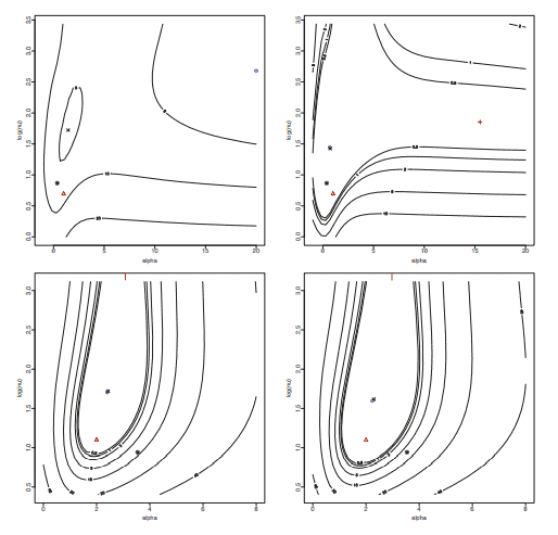
Several simulations runs have been performed to examine the performance of the proposed methodology. The computing environment was $\mathrm{R}$ version 3.6.0. The reference point for these evaluations is the methodology currently in use, as provided by the publicly available version of $R$ package $s n$ at the time of writing, namely version 1.5-4; see Azzalini (2019). This will be denoted ‘the current method’ in the following. Since the role of the proposed method is to initialize the numerical MLE search, not the initialization procedure per se, we compare the new and the current method with respect to final MLE outcome. However, since the numerical optimization method used after initialization is the same, any variations in the results originate from the different initialization procedures.

We stress again that in a vast number of cases the working of the current method is satisfactory and we are aiming at improvements when dealing with ‘awkward samples’. These commonly arise with ST distributions having low degrees of freedom, about $v=1$ or even less, but exceptions exist, such as the second sample in Fig. $2 .$

The primary aspect of interest is improvement in the quality of data fitting. This is typically expressed as an increase of the maximal achieved log-likelihood, in its penalized form. Another desirable effect is improvement in computing time.

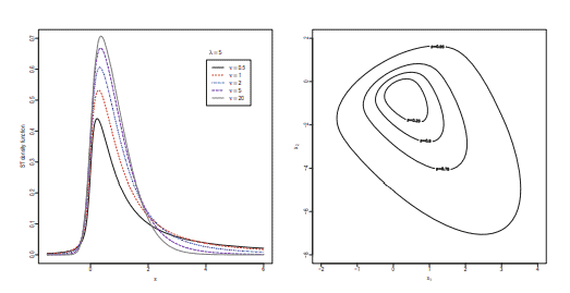
The basic set-up for such numerical experiments is represented by simple random samples, obtained as independent and identically distributed values drawn from a named ST $(\xi, \omega, \lambda, v)$. In all cases we set $\xi=0$ and $\omega=1$. For the other ingredients, we have selected the following values:
$\lambda: 0, \quad 2, \quad 8$,
$v: 1,3,8$,
$n: 50,100,250,500$
and, for each combination of these values, $N=2000$ samples have been drawn.
The smallest examined sample size, $n=50$, must be regarded as a sort of ‘sensible lower bound’ for realistic fitting of flexible distributions such as the ST. In this respect, recall the cautionary note of Azzalini and Capitanio (2014, p. 63) about the fitting of a SN distribution with small sample sizes. Since the ST involves an additional parameter, notably one having a strong effect on tail behaviour, that annotation holds a fortiori here.

For each of the $3 \times 3 \times 4 \times 2000=72,000$ samples so generated, estimation of the parameters $(\xi, \omega, \lambda, \nu)$ has been carried out using the following methods.

统计代写|生物统计代写biostatistics代考|MPH701

生物统计代考

统计代写|生物统计代写biostatistics代考|Extension to the Regression Case

我们想扩展 Sect 的方法论。3.2回归设置,其中位置参数随观测值变化,作为一组线性函数p,比如说,假设包括常数项的解释变量,因为它通常是这种情况。如果X一世是与一世主题,观察是一世现在假设从 ST 中提取(X一世,ω,λ,ν)在哪里

X一世=X一世⊤b,一世=1,…,n,
对于一些p维向量b未知参数;因此现在参数向量是θ=(b⊤,ω,λ,在)⊤. 保留独立绘制观察的假设。

中值的直接扩展作为位置的估计,在 Sect. 3.2,是一个估计b通过中值回归获得,这对应于采用最小绝对偏差拟合标准而不是更熟悉的最小二乘法。当分位数水平设置为1/2. 分位数回归的经典处理

是 Koenker (2005),相应的数值工作可以使用Rquantreg 包,请参阅 Koenker (2018) 等工具。

使用中值回归提供估计b~~米的b和一个残差向量,r一世=是一世−X一世⊤b~米为了一世=1,…,n. 忽略b估计误差,这些残差是从小号吨(−米0,ω2,λ,在), 在哪里米0是一个合适的值,很快就会检查,这使得分布的中位数为 0,因为这是中位数回归标准的目标。然后我们可以使用 Sect 的相同程序。3.2,与是一世取代了r一世的,估计ω,λ,在,给定的值米0在这个阶段是无关紧要的。

最后一步是对向量的修正b~米调整的事实是一世−X一世⊤b应该有中位数米0,即 ST 的中位数(0,ω,λ,在),而不是中位数 0 。这相当于将所有残差增加一个恒定值米0, 这一步是通过设置一个向量来完成的b~所有组件都等于 tōb~米除了截距项,b0说,估计是

b~0=b~0米−ω~q2小号吨
类似于(10)

统计代写|生物统计代写biostatistics代考|Extension to the Multivariate Case

现在考虑以下情况n来自多变量的独立观察是随密度 (6) 变化,因此是∼小号吨d(X,Ω,一个,在). 这种情况可以结合Sect的回归设置。3.3,因此d- 维位置参数根据每个观察值变化

X一世⊤=X一世⊤b,一世=1,…,n,
现在在哪里b=(b⋅1,…,b⋅d)是一个p×d参数矩阵。由于我们假设解释变量包括一个常数项,回归情况包含相同分布的情况,当p=1. 因此,我们直接处理回归情况,其中一世第一次观察是从是一世∼ 小号吨d(X一世,Ω,一个,在)和X一世由 (12) 给出,对于一世=1,…,n.

将观测值排列在一个n×d矩阵是=(是一世j). 应用程序中介绍的部分。3.2和3.3分别到每一列是提供估计d单变量模型。具体来说,从j第 列是, 我们得到估计θ~j和相应的“归一化”残差和~一世j :

θ~j=(b~⋅j⊤,ω~j,λ~j,在~j)⊤,和~一世j=ω~j−1(是一世j−X一世⊤b~⋅j)

必须记住,“归一化”操作使用位置和尺度参数,但这些参数与基础随机变量的均值和标准差不一致。

由于表达式 (12) 的含义是定义一组具有共同设计矩阵的单变量回归模式,因此向量b~−1,…,b~⋅d可以简单地排列成一个p×d矩阵b~这代表了一个估计b.

(13)中的一组单变量估计提供d估计为在,而只有一个这样的值进入多元 ST 分布的规范。我们采用了 $\tilde{v} {1}、\ldots、\tilde{v} {d}的中位数一个s吨H和s一世nGl和r和q在一世r和d和s吨一世米一个吨和,d和n○吨和d\波浪号 {v} $。

规模数量ω~1,…,ω~d估计对角线元素的平方根Ω,但非对角线元素需要单独的估计步骤。真正需要估计的是无标度矩阵Ω¯. 这是接下来要研究的问题。

如果ω是由的平方根形成的对角矩阵Ω11,…,Ω分类 , 所有变量ω−1(是一世−X一世)有分布小号吨d(0,Ω¯,一个,在), 为了一世=1,…,n. 表示为从=(从1,…,从d)⊤这组变量的通用成员。我们关心产品的分销从j从ķ,但为了符号的简单性,我们专注于特定的产品在=从1从2,因为所有其他产品都具有相似的性质。

然后我们必须检查分布在=从1从2什么时候(从1,从2)是一个二元 ST 变量。起初这看起来是一项艰巨的任务,但考虑到对称调制分布的扰动不变性特性,提供了一个主要的简化,ST 就是其中的一个例子。有关此属性的精确说明,请参见例如 Proposition1.4Azzalini 和 Capitanio (2014),但在目前的情况下,它说,因为在是一个偶函数(从1,从2), 它的分布不依赖于一个,并且与案例的分布相吻合一个=0,即通常的双变量学生的情况吨分布,具有依赖参数Ω¯12.

统计代写|生物统计代写biostatistics代考|Simulation Work to Compare Initialization Procedures

已经进行了几次模拟运行以检查所提出的方法的性能。计算环境是R版本 3.6.0。这些评估的参考点是当前使用的方法,由公开版本提供R包裹sn在撰写本文时,即版本 1.5-4;见阿扎里尼 (2019)。这将在下文中表示为“当前方法”。由于所提出方法的作用是初始化数值 MLE 搜索,而不是初始化过程本身,我们比较新方法和当前方法的最终 MLE 结果。但是,由于初始化后使用的数值优化方法是相同的,因此结果的任何变化都源于不同的初始化程序。

我们再次强调,在大量情况下,当前方法的工作是令人满意的,我们的目标是在处理“尴尬样本”时进行改进。这些通常出现在具有低自由度的 ST 分布中,大约在=1甚至更少,但也有例外,例如图 2 中的第二个示例。2.

感兴趣的主要方面是数据拟合质量的改进。这通常以惩罚形式表示为最大实现对数似然的增加。另一个理想的效果是计算时间的改进。

此类数值实验的基本设置由简单的随机样本表示,这些样本是从命名的 ST 中提取的独立且同分布的值(X,ω,λ,在). 在所有情况下,我们设置X=0和ω=1. 对于其他成分,我们选择了以下值:
λ:0,2,8,
在:1,3,8,
n:50,100,250,500
并且,对于这些值的每种组合,ñ=2000样本已抽取。
最小的检查样本量,n=50, 必须被视为一种“合理的下界”,用于实际拟合灵活分布(例如 ST)。在这方面,回想一下 Azzalini 和 Capitanio (2014, p. 63) 关于在小样本量下拟合 SN 分布的警告说明。由于 ST 涉及一个附加参数,尤其是对尾部行为有强烈影响的参数,因此该注释在这里更重要。

对于每一个3×3×4×2000=72,000这样生成的样本,参数的估计(X,ω,λ,ν)已使用以下方法进行。

统计代写|生物统计代写biostatistics代考 请认准statistics-lab™

统计代写请认准statistics-lab™. statistics-lab™为您的留学生涯保驾护航。

金融工程代写

金融工程是使用数学技术来解决金融问题。金融工程使用计算机科学、统计学、经济学和应用数学领域的工具和知识来解决当前的金融问题,以及设计新的和创新的金融产品。

非参数统计代写

非参数统计指的是一种统计方法,其中不假设数据来自于由少数参数决定的规定模型;这种模型的例子包括正态分布模型和线性回归模型。

广义线性模型代考

广义线性模型(GLM)归属统计学领域,是一种应用灵活的线性回归模型。该模型允许因变量的偏差分布有除了正态分布之外的其它分布。

术语 广义线性模型(GLM)通常是指给定连续和/或分类预测因素的连续响应变量的常规线性回归模型。它包括多元线性回归,以及方差分析和方差分析(仅含固定效应)。

有限元方法代写

有限元方法(FEM)是一种流行的方法,用于数值解决工程和数学建模中出现的微分方程。典型的问题领域包括结构分析、传热、流体流动、质量运输和电磁势等传统领域。

有限元是一种通用的数值方法,用于解决两个或三个空间变量的偏微分方程(即一些边界值问题)。为了解决一个问题,有限元将一个大系统细分为更小、更简单的部分,称为有限元。这是通过在空间维度上的特定空间离散化来实现的,它是通过构建对象的网格来实现的:用于求解的数值域,它有有限数量的点。边界值问题的有限元方法表述最终导致一个代数方程组。该方法在域上对未知函数进行逼近。[1] 然后将模拟这些有限元的简单方程组合成一个更大的方程系统,以模拟整个问题。然后,有限元通过变化微积分使相关的误差函数最小化来逼近一个解决方案。

tatistics-lab作为专业的留学生服务机构,多年来已为美国、英国、加拿大、澳洲等留学热门地的学生提供专业的学术服务,包括但不限于Essay代写,Assignment代写,Dissertation代写,Report代写,小组作业代写,Proposal代写,Paper代写,Presentation代写,计算机作业代写,论文修改和润色,网课代做,exam代考等等。写作范围涵盖高中,本科,研究生等海外留学全阶段,辐射金融,经济学,会计学,审计学,管理学等全球99%专业科目。写作团队既有专业英语母语作者,也有海外名校硕博留学生,每位写作老师都拥有过硬的语言能力,专业的学科背景和学术写作经验。我们承诺100%原创,100%专业,100%准时,100%满意。

随机分析代写


随机微积分是数学的一个分支,对随机过程进行操作。它允许为随机过程的积分定义一个关于随机过程的一致的积分理论。这个领域是由日本数学家伊藤清在第二次世界大战期间创建并开始的。

时间序列分析代写

随机过程,是依赖于参数的一组随机变量的全体,参数通常是时间。 随机变量是随机现象的数量表现,其时间序列是一组按照时间发生先后顺序进行排列的数据点序列。通常一组时间序列的时间间隔为一恒定值(如1秒,5分钟,12小时,7天,1年),因此时间序列可以作为离散时间数据进行分析处理。研究时间序列数据的意义在于现实中,往往需要研究某个事物其随时间发展变化的规律。这就需要通过研究该事物过去发展的历史记录,以得到其自身发展的规律。

回归分析代写

多元回归分析渐进(Multiple Regression Analysis Asymptotics)属于计量经济学领域,主要是一种数学上的统计分析方法,可以分析复杂情况下各影响因素的数学关系,在自然科学、社会和经济学等多个领域内应用广泛。

MATLAB代写

MATLAB 是一种用于技术计算的高性能语言。它将计算、可视化和编程集成在一个易于使用的环境中,其中问题和解决方案以熟悉的数学符号表示。典型用途包括:数学和计算算法开发建模、仿真和原型制作数据分析、探索和可视化科学和工程图形应用程序开发,包括图形用户界面构建MATLAB 是一个交互式系统,其基本数据元素是一个不需要维度的数组。这使您可以解决许多技术计算问题,尤其是那些具有矩阵和向量公式的问题,而只需用 C 或 Fortran 等标量非交互式语言编写程序所需的时间的一小部分。MATLAB 名称代表矩阵实验室。MATLAB 最初的编写目的是提供对由 LINPACK 和 EISPACK 项目开发的矩阵软件的轻松访问,这两个项目共同代表了矩阵计算软件的最新技术。MATLAB 经过多年的发展,得到了许多用户的投入。在大学环境中,它是数学、工程和科学入门和高级课程的标准教学工具。在工业领域,MATLAB 是高效研究、开发和分析的首选工具。MATLAB 具有一系列称为工具箱的特定于应用程序的解决方案。对于大多数 MATLAB 用户来说非常重要,工具箱允许您学习应用专业技术。工具箱是 MATLAB 函数(M 文件)的综合集合,可扩展 MATLAB 环境以解决特定类别的问题。可用工具箱的领域包括信号处理、控制系统、神经网络、模糊逻辑、小波、仿真等。

R语言代写问卷设计与分析代写
PYTHON代写回归分析与线性模型代写
MATLAB代写方差分析与试验设计代写
STATA代写机器学习/统计学习代写
SPSS代写计量经济学代写
EVIEWS代写时间序列分析代写
EXCEL代写深度学习代写
SQL代写各种数据建模与可视化代写

统计代写|生物统计代写biostatistics代考|STA 310

如果你也在 怎样代写生物统计biostatistics这个学科遇到相关的难题,请随时右上角联系我们的24/7代写客服。

生物统计学是将统计技术应用于健康相关领域的科学研究,包括医学、生物学和公共卫生,并开发新的工具来研究这些领域。

statistics-lab™ 为您的留学生涯保驾护航 在代写生物统计biostatistics方面已经树立了自己的口碑, 保证靠谱, 高质且原创的统计Statistics代写服务。我们的专家在代写生物统计biostatistics代写方面经验极为丰富,各种生物统计biostatistics相关的作业也就用不着说。

我们提供的生物统计biostatistics及其相关学科的代写,服务范围广, 其中包括但不限于:

  • Statistical Inference 统计推断
  • Statistical Computing 统计计算
  • Advanced Probability Theory 高等概率论
  • Advanced Mathematical Statistics 高等数理统计学
  • (Generalized) Linear Models 广义线性模型
  • Statistical Machine Learning 统计机器学习
  • Longitudinal Data Analysis 纵向数据分析
  • Foundations of Data Science 数据科学基础
统计代写|生物统计代写biostatistics代考|STA 310

统计代写|生物统计代写biostatistics代考|Numerical Aspects and Some Illustrations

Since, on the computational side, we shall base our work the R package sn, described by Azzalini (2019), it is appropriate to describe some key aspects of this package. There exists a comprehensive function for model fitting, called selm, but the actual numerical work in case of an ST model is performed by functions st. mple and mst. mple, in the univariate and the multivariate case, respectively. To numerical efficiency, we shall be using these functions directly, rather than via selm. As their names suggest, st. mple and mst. mple perform MPLE, but they can be used for classical MLE as well, just by omitting the penalty function. The rest of the description refers to st. mple, but mst. mple follows a similar scheme.
In the univariate case, denote by $\theta=(\xi, \omega, \alpha, \nu)^{\top}$ the parameters to be cstimatcd, or possibly $\theta=\left(\beta^{\top}, w, \alpha, v\right)^{\top}$ when a lincar regrcssion mudel is introduced for the location parameter, in which case $\beta$ is a vector of $p$ regression coefficients. Denote by $\log L(\theta)$ the log-likelihood function at point $\theta$. If no starting values are supplied, the first operation of st.mple is to fit a linear model to the available explanatory variables; this reduces to the constant covariate value 1 if $p=1$. For the residuals from this linear fit, sample cumulants of order up to four are computed, hence including the sample variance. An inversion from these

values to $\theta$ may or may not be possible, depending on whether the third and fourth sample cumulants fall in the feasible region for the ST family. If the inversion is successful, initial values of the parameters are so obtained; if not, the final two components of $\theta$ are set at $(\alpha, v)=(0,10)$, retaining the other components from the linear fit. Starting from this point, MLE or MPLE is searched for using a general numerical optimization procedure. The default procedure for performing this step is the $\mathrm{R}$ function nlminb, supplied with the score functions besides the log-likelihood function. We shall refer, comprehensively, to this currently standard procedure as ‘method M0’.

In all our numerical work, method M0 uses st. mple, and the involved function nlminb, with all tuning parameters kept at their default values. The only activated option is the one switching between MPLE and MLE, and even this only for the work of the present section. Later on, we shall always use MPLE, with penalty function Openalty which implements the method proposed in Azzalini and Arellano-Valle (2013).

We start our numerical work with some illustrations, essentially in graphical form, of the log-likelihood generated by some simulated datasets. The aim is to provide a direct perception, although inevitably limited, of the possible behaviour of the log-likelihood and the ensuing problems which it poses for MLE search and other inferential procedures. Given this aim, we focus on cases which are unusual, in some way or another, rather than on ‘plain cases’.

The type of graphical display which we adopt is based on the profile loglikelihood function of $(\alpha, v)$, denoted $\log L_{p}(\alpha, v)$. This is obtained, for any given $(\alpha, v)$, by maximizing $\log L(\theta)$ with respect to the remaining parameters. To simplify readability, we transform $\log L_{p}(\alpha, v)$ to the likelihood ratio test statistic, also called ‘deviance function’:
$$
D(\alpha, v)=2\left{\log L_{p}(\hat{\alpha}, \hat{v})-\log L_{p}(\alpha, v)\right}
$$
where $\log L_{p}(\hat{\alpha}, \hat{v})$ is the overall maximum value of the log-likelihood, equivalent to $\log L(\hat{\theta})$. The concept of deviance applies equally to the penalized log-likelihood.
The plots in Fig. 2 displays, in the form of contour level plots, the behaviour of $D(\alpha, v)$ for two artificially generated samples, with $v$ expressed on the logarithmic scale for more convenient readability. Specifically, the top plots refer to a sample of size $n=50$ drawn from the $\operatorname{ST}(0,1,1,2)$; the left plot, refers to the regular log-likelihood, while the right plot refers to the penalized log-likelihood. The plots include marks for points of special interest, as follows:
$\Delta$ the true parameter point;
o the point having maximal (penalized) log-likelihood on a $51 \times 51$ grid of points spanning the plotted area;

  • the MLE or MPLE point selected by method M0;
  • the preliminary estimate to be introduced in Sect. 3.2, later denoted M1;
    $\times$ the MLE or MPLE point selected by method M2 presented later in the text.

统计代写|生物统计代写biostatistics代考|Preliminary Remarks and the Basic Scheme

We have seen in Sect. 2 the ST log-likelihood function can be problematic; it is then advisable to select carefully the starting point for the MLE search. While contrasting the risk of landing on a local maximum, a connected aspect of interest is to reduce the overall computing time. Here are some preliminary considerations about the stated target.

Since these initial estimates will be refined by a subsequent step of log-likelihood maximization, there is no point in aiming at a very sophisticate method. In addition, we want to keep the involved computing header as light as possible. Therefore, we want a method which is simple and quick to compute; at the same time, it should be reasonably reliable, hopefully avoiding nonsensical outcomes.

Another consideration is that we cannot work with the methods of moments, or some variant of it, as this would impose a condition $v>4$, bearing in mind the constraints recalled in Sect. 1.2. Since some of the most interesting applications of ST-based models deal with very heavy tails, hence with low degrees of freedom, the condition $v>4$ would be unacceptable in many important applications. The implication is that we have to work with quantiles and derived quantities.

To ease exposition, we begin by presenting the logic in the basic case of independent observations from a common univariate distribution $\mathrm{ST}\left(\xi, \omega^{2}, \lambda, v\right)$. The first step is to select suitable quantile-based measures of location, scale,

asymmetry and tail-weight. The following list presents a set of reasonable choices; these measures can be equally referred to a probability distribution or to a sample, depending on the interpretation of the terms quantile, quartile and alike.

Location The median is the obvious choice here; denote it by $q_{2}$, since it coincides with the second quartile.

Scale A commonly used measure of scale is the semi-interquartile difference, also called quartile deviation, that is
$$
d_{q}=\frac{1}{2}\left(q_{3}-q_{1}\right)
$$
where $q_{j}$ denotes the $j$ th quartile; see for instance Kotz et al. (2006, vol. 10, p. 6743).

Asymmetry A classical non-parametric measure of asymmetry is the so-called Bowley’s measure
$$
G=\frac{\left(q_{3}-q_{2}\right)-\left(q_{2}-q_{1}\right)}{q_{3}-q_{1}}=\frac{q_{3}-2 q_{2}+q_{1}}{2 d_{q}}
$$
see Kotz et al. (2006, vol. 12, p. 7771-3). Since the same quantity, up to an inessential difference, had previously been used by Galton, some authors attribute to him its introduction. We shall refer to $G$ as the Galton-Bowley measure.

Kurtosis A relatively more recent proposal is the Moors measure of kurtosis, presented in Moors (1988),
$$
M=\frac{\left(e_{7}-e_{5}\right)+\left(e_{3}-e_{1}\right)}{e_{6}-e_{2}}
$$
where $e_{j}$ denotes the $j$ th octile, for $j=1, \ldots, 7$. Clearly, $e_{2 j}=q_{j}$ for $j=$ $1,2,3$

统计代写|生物统计代写biostatistics代考|Inversion of Quantile-Based Measures to ST Parameters

For the inversion of the parameter set $Q=\left(q_{2}, d_{q}, G, M\right)$ to $\theta=(\xi, \omega, \lambda, v)$, the first stage considers only the components $(G, M)$ which are to be mapped to $(\lambda, v)$, exploiting the invariance of $G$ and $M$ with respect to location and scale. Hence, at this stage, we can work assuming that $\xi=0$ and $\omega=1$.

Start by computing, for any given pair $(\lambda, v)$, the set of octiles $e_{1}, \ldots, e_{7}$ of $\mathrm{ST}(0,1, \lambda, v)$, and from here the corresponding $(G, M)$ values. Operationally, we have computed the ST quantiles using routine qst of package sn. Only nonnegative values of $\lambda$ need to be considered, because a reversal of the $\lambda$ sign simply reverses the sign of $G$, while $M$ is unaffected, thanks to the mirroring property of the ST quantiles when $\lambda$ is changed to $-\lambda$.

Initially, our numerical exploration of the inversion process examined the contour level plots of $G$ and $M$ as functions of $\lambda$ and $v$, as this appeared to be the more natural approach. Unfortunately, these plots turned out not to be useful, because of the lack of a sufficiently regular pattern of the contour curves. Therefore these plots are not even displayed here.

A more useful display is the one adopted in Fig. 3, where the coordinate axes are now $G$ and $M$. The shaded area, which is the same in both panels, represents the set of feasible $(G, M)$ points for the ST family. In the first plot, each of the black lines indicates the locus of points with constant values of $\delta$, defined by (4), when $v$ spans the positive half-line; the selected $\delta$ values are printed at the top of the shaded area, when feasible without clutter of the labels. The use of $\delta$ instead of $\lambda$ simply yields a better spread of the contour lines with different parameter values, but it is conceptually irrelevant. The second plot of Fig. 3 displays the same admissible region with superimposed a different type of loci, namely those corresponding to specified values of $v$, when $\delta$ spans the $[0,1]$ interval; the selected $v$ values are printed on the left side of the shaded area.

Details of the numerical calculations are as follows. The Galton-Bowley and the Moors measures have been evaluated over a $13 \times 25$ grid of points identified by the selected values
$$
\begin{aligned}
\delta^{}=&(0,0.1,0.2,0.3,0.4,0.5,0.6,0.7,0.8,0.9,0.95,0.99,1) \ v^{}=&(0.30,0.32,0.35,0.40,0.45,0.50,0.60,0.70,0.80,0.90,1,1.5,2\
&3,4,5,7,10,15,20,30,40,50,100, \infty)
\end{aligned}
$$

统计代写|生物统计代写biostatistics代考|STA 310

生物统计代考

统计代写|生物统计代写biostatistics代考|Numerical Aspects and Some Illustrations

由于在计算方面,我们的工作将基于 Azzalini (2019) 描述的 R 包 sn,因此描述该包的一些关键方面是合适的。存在一个用于模型拟合的综合函数,称为 selm,但在 ST 模型的情况下,实际数值工作由函数 st 执行。mple 和 mst。mple,分别在单变量和多变量情况下。为了数值效率,我们将直接使用这些函数,而不是通过 selm。正如他们的名字所暗示的那样,圣。mple 和 mst。mple 执行 MPLE,但它们也可以用于经典 MLE,只需省略惩罚函数。其余的描述指的是圣。mple,但mst。mple 遵循类似的方案。
在单变量情况下,表示为θ=(X,ω,一个,ν)⊤要 cstimatcd 的参数,或者可能θ=(b⊤,在,一个,在)⊤当为位置参数引入 lincar rercssion mudel 时,在这种情况下b是一个向量p回归系数。表示为日志⁡大号(θ)点的对数似然函数θ. 如果没有提供起始值,则 st.mple 的第一个操作是将线性模型拟合到可用的解释变量;这减少到常数协变量值 1 如果p=1. 对于这种线性拟合的残差,计算最多四阶的样本累积量,因此包括样本方差。从这些倒置

值到θ可能或不可能,取决于第三个和第四个样本累积量是否落在 ST 系列的可行区域内。如果反演成功,则得到参数的初始值;如果没有,最后两个组件θ设置在(一个,在)=(0,10),保留线性拟合中的其他分量。从这一点开始,使用一般数值优化程序搜索 MLE 或 MPLE。执行此步骤的默认程序是R函数 nlminb,除了对数似然函数外,还提供分数函数。我们将把这个目前的标准程序统称为“方法 M0”。

在我们所有的数值工作中,方法 M0 使用 st。mple 和涉及的函数 nlminb,所有调整参数都保持在默认值。唯一激活的选项是在 MPLE 和 MLE 之间切换,甚至这仅适用于本节的工作。稍后,我们将始终使用带有惩罚函数 Openalty 的 MPLE,它实现了 Azzalini 和 Arellano-Valle (2013) 中提出的方法。

我们从一些模拟数据集生成的对数似然的插图开始我们的数值工作,基本上以图形形式。目的是提供对数似然的可能行为以及它为 MLE 搜索和其他推理过程带来的后续问题的直接感知,尽管不可避免地受到限制。鉴于这一目标,我们专注于以某种方式不寻常的案件,而不是“普通案件”。

我们采用的图形显示类型是基于轮廓对数似然函数(一个,在), 表示日志⁡大号p(一个,在). 这是获得的,对于任何给定的(一个,在),通过最大化日志⁡大号(θ)关于其余参数。为了简化可读性,我们将日志⁡大号p(一个,在)似然比检验统计量,也称为“偏差函数”:

D(\alpha, v)=2\left{\log L_{p}(\hat{\alpha}, \hat{v})-\log L_{p}(\alpha, v)\right}D(\alpha, v)=2\left{\log L_{p}(\hat{\alpha}, \hat{v})-\log L_{p}(\alpha, v)\right}
在哪里日志⁡大号p(一个^,在^)是对数似然的整体最大值,相当于日志⁡大号(θ^). 偏差的概念同样适用于惩罚对数似然。
图 2 中的图以等高线水平图的形式显示了D(一个,在)对于两个人工生成的样本,在以对数刻度表示,以便于阅读。具体来说,上面的图是指一个大小的样本n=50取自英石⁡(0,1,1,2); 左图是指常规对数似然,而右图是指惩罚对数似然。这些图包括特殊兴趣点的标记,如下所示:
Δ真正的参数点;
o 在 a 上具有最大(惩罚)对数似然的点51×51跨越绘图区域的点网格;

  • 方法 M0 选择的 MLE 或 MPLE 点;
  • 将在 Sect 中介绍的初步估计。3.2,后面记为M1;
    ×文中稍后介绍的方法 M2 选择的 MLE 或 MPLE 点。

统计代写|生物统计代写biostatistics代考|Preliminary Remarks and the Basic Scheme

我们在教派中见过。2 ST 对数似然函数可能有问题;然后建议仔细选择 MLE 搜索的起点。在对比着陆到局部最大值的风险时,感兴趣的一个相关方面是减少整体计算时间。以下是关于既定目标的一些初步考虑。

由于这些初始估计将通过对数似然最大化的后续步骤进行细化,因此以非常复杂的方法为目标是没有意义的。此外,我们希望使所涉及的计算头尽可能轻。因此,我们需要一种简单快速计算的方法;同时,它应该是相当可靠的,希望能避免无意义的结果。

另一个考虑是,我们不能使用矩量方法或它的一些变体,因为这会强加一个条件在>4,牢记 Sect 中回忆的约束。1.2. 由于基于 ST 的模型的一些最有趣的应用处理非常重的尾部,因此具有低自由度,条件在>4在许多重要应用中是不可接受的。这意味着我们必须使用分位数和派生数量。

为了便于说明,我们首先介绍来自共同单变量分布的独立观察的基本情况下的逻辑小号吨(X,ω2,λ,在). 第一步是选择合适的基于分位数的位置、规模、

不对称和尾重。下面列出了一组合理的选择;根据对分位数、四分位数等术语的解释,这些度量可以同样称为概率分布或样本。

位置 中位数是这里的明显选择;表示为q2,因为它与第二个四分位数一致。

尺度 常用的尺度度量是半四分位差,也称为四分位差,即

dq=12(q3−q1)
在哪里qj表示j第四分位数;例如,参见 Kotz 等人。(2006 年,第 10 卷,第 6743 页)。

不对称 不对称的经典非参数度量是所谓的鲍利度量

G=(q3−q2)−(q2−q1)q3−q1=q3−2q2+q12dq
参见 Kotz 等人。(2006 年,第 12 卷,第 7771-3 页)。由于高尔顿之前使用了相同的数量,但存在无关紧要的差异,因此一些作者将其归因于他的介绍。我们将参考G作为 Galton-Bowley 度量。

峰度 一个相对较新的建议是 Moors 峰度测量,在 Moors (1988) 中提出,

米=(和7−和5)+(和3−和1)和6−和2
在哪里和j表示j八分位数,对于j=1,…,7. 清楚地,和2j=qj为了j= 1,2,3

统计代写|生物统计代写biostatistics代考|Inversion of Quantile-Based Measures to ST Parameters

对于参数集的反演问=(q2,dq,G,米)至θ=(X,ω,λ,在),第一阶段只考虑组件(G,米)要映射到的(λ,在),利用不变性G和米关于位置和规模。因此,在这个阶段,我们可以假设X=0和ω=1.

从计算开始,对于任何给定的对(λ,在), 八分位数的集合和1,…,和7的小号吨(0,1,λ,在),从这里对应的(G,米)价值观。在操作上,我们使用包 sn 的例程 qst 计算了 ST 分位数。只有非负值λ需要考虑,因为逆转λ符号只是反转符号G, 尽管米不受影响,这要归功于 ST 分位数的镜像属性,当λ改为−λ.

最初,我们对反演过程的数值探索检查了等值线水平图G和米作为函数λ和在,因为这似乎是更自然的方法。不幸的是,这些图没有用,因为轮廓曲线缺乏足够规则的图案。因此,这些图甚至没有在这里显示。

更有用的显示是图 3 中采用的显示,其中坐标轴现在是G和米. 两个面板中相同的阴影区域表示可行的集合(G,米)ST家族的积分。在第一个图中,每条黑线表示具有常数值的点的轨迹d,由 (4) 定义,当在跨越正半线;被选中的d值打印在阴影区域的顶部,如果可行,标签不会混乱。指某东西的用途d代替λ简单地产生具有不同参数值的等高线的更好分布,但它在概念上无关紧要。图 3 的第二个图显示了相同的允许区域,其中叠加了不同类型的基因座,即对应于指定值的基因座在, 什么时候d跨越[0,1]间隔; 被选中的在值打印在阴影区域的左侧。

数值计算的细节如下。Galton-Bowley 和 Moors 措施已经过评估13×25由所选值标识的点网格

统计代写|生物统计代写biostatistics代考 请认准statistics-lab™

统计代写请认准statistics-lab™. statistics-lab™为您的留学生涯保驾护航。

金融工程代写

金融工程是使用数学技术来解决金融问题。金融工程使用计算机科学、统计学、经济学和应用数学领域的工具和知识来解决当前的金融问题,以及设计新的和创新的金融产品。

非参数统计代写

非参数统计指的是一种统计方法,其中不假设数据来自于由少数参数决定的规定模型;这种模型的例子包括正态分布模型和线性回归模型。

广义线性模型代考

广义线性模型(GLM)归属统计学领域,是一种应用灵活的线性回归模型。该模型允许因变量的偏差分布有除了正态分布之外的其它分布。

术语 广义线性模型(GLM)通常是指给定连续和/或分类预测因素的连续响应变量的常规线性回归模型。它包括多元线性回归,以及方差分析和方差分析(仅含固定效应)。

有限元方法代写

有限元方法(FEM)是一种流行的方法,用于数值解决工程和数学建模中出现的微分方程。典型的问题领域包括结构分析、传热、流体流动、质量运输和电磁势等传统领域。

有限元是一种通用的数值方法,用于解决两个或三个空间变量的偏微分方程(即一些边界值问题)。为了解决一个问题,有限元将一个大系统细分为更小、更简单的部分,称为有限元。这是通过在空间维度上的特定空间离散化来实现的,它是通过构建对象的网格来实现的:用于求解的数值域,它有有限数量的点。边界值问题的有限元方法表述最终导致一个代数方程组。该方法在域上对未知函数进行逼近。[1] 然后将模拟这些有限元的简单方程组合成一个更大的方程系统,以模拟整个问题。然后,有限元通过变化微积分使相关的误差函数最小化来逼近一个解决方案。

tatistics-lab作为专业的留学生服务机构,多年来已为美国、英国、加拿大、澳洲等留学热门地的学生提供专业的学术服务,包括但不限于Essay代写,Assignment代写,Dissertation代写,Report代写,小组作业代写,Proposal代写,Paper代写,Presentation代写,计算机作业代写,论文修改和润色,网课代做,exam代考等等。写作范围涵盖高中,本科,研究生等海外留学全阶段,辐射金融,经济学,会计学,审计学,管理学等全球99%专业科目。写作团队既有专业英语母语作者,也有海外名校硕博留学生,每位写作老师都拥有过硬的语言能力,专业的学科背景和学术写作经验。我们承诺100%原创,100%专业,100%准时,100%满意。

随机分析代写


随机微积分是数学的一个分支,对随机过程进行操作。它允许为随机过程的积分定义一个关于随机过程的一致的积分理论。这个领域是由日本数学家伊藤清在第二次世界大战期间创建并开始的。

时间序列分析代写

随机过程,是依赖于参数的一组随机变量的全体,参数通常是时间。 随机变量是随机现象的数量表现,其时间序列是一组按照时间发生先后顺序进行排列的数据点序列。通常一组时间序列的时间间隔为一恒定值(如1秒,5分钟,12小时,7天,1年),因此时间序列可以作为离散时间数据进行分析处理。研究时间序列数据的意义在于现实中,往往需要研究某个事物其随时间发展变化的规律。这就需要通过研究该事物过去发展的历史记录,以得到其自身发展的规律。

回归分析代写

多元回归分析渐进(Multiple Regression Analysis Asymptotics)属于计量经济学领域,主要是一种数学上的统计分析方法,可以分析复杂情况下各影响因素的数学关系,在自然科学、社会和经济学等多个领域内应用广泛。

MATLAB代写

MATLAB 是一种用于技术计算的高性能语言。它将计算、可视化和编程集成在一个易于使用的环境中,其中问题和解决方案以熟悉的数学符号表示。典型用途包括:数学和计算算法开发建模、仿真和原型制作数据分析、探索和可视化科学和工程图形应用程序开发,包括图形用户界面构建MATLAB 是一个交互式系统,其基本数据元素是一个不需要维度的数组。这使您可以解决许多技术计算问题,尤其是那些具有矩阵和向量公式的问题,而只需用 C 或 Fortran 等标量非交互式语言编写程序所需的时间的一小部分。MATLAB 名称代表矩阵实验室。MATLAB 最初的编写目的是提供对由 LINPACK 和 EISPACK 项目开发的矩阵软件的轻松访问,这两个项目共同代表了矩阵计算软件的最新技术。MATLAB 经过多年的发展,得到了许多用户的投入。在大学环境中,它是数学、工程和科学入门和高级课程的标准教学工具。在工业领域,MATLAB 是高效研究、开发和分析的首选工具。MATLAB 具有一系列称为工具箱的特定于应用程序的解决方案。对于大多数 MATLAB 用户来说非常重要,工具箱允许您学习应用专业技术。工具箱是 MATLAB 函数(M 文件)的综合集合,可扩展 MATLAB 环境以解决特定类别的问题。可用工具箱的领域包括信号处理、控制系统、神经网络、模糊逻辑、小波、仿真等。

R语言代写问卷设计与分析代写
PYTHON代写回归分析与线性模型代写
MATLAB代写方差分析与试验设计代写
STATA代写机器学习/统计学习代写
SPSS代写计量经济学代写
EVIEWS代写时间序列分析代写
EXCEL代写深度学习代写
SQL代写各种数据建模与可视化代写

统计代写|生物统计代写biostatistics代考|BIOL 220

如果你也在 怎样代写生物统计biostatistics这个学科遇到相关的难题,请随时右上角联系我们的24/7代写客服。

生物统计学是将统计技术应用于健康相关领域的科学研究,包括医学、生物学和公共卫生,并开发新的工具来研究这些领域。

statistics-lab™ 为您的留学生涯保驾护航 在代写生物统计biostatistics方面已经树立了自己的口碑, 保证靠谱, 高质且原创的统计Statistics代写服务。我们的专家在代写生物统计biostatistics代写方面经验极为丰富,各种生物统计biostatistics相关的作业也就用不着说。

我们提供的生物统计biostatistics及其相关学科的代写,服务范围广, 其中包括但不限于:

  • Statistical Inference 统计推断
  • Statistical Computing 统计计算
  • Advanced Probability Theory 高等概率论
  • Advanced Mathematical Statistics 高等数理统计学
  • (Generalized) Linear Models 广义线性模型
  • Statistical Machine Learning 统计机器学习
  • Longitudinal Data Analysis 纵向数据分析
  • Foundations of Data Science 数据科学基础
统计代写|生物统计代写biostatistics代考|BIOL 220

统计代写|生物统计代写biostatistics代考|Flexible Distributions: The Skew-t Case

In the context of distribution theory, a central theme is the study of flexible parametric families of probability distributions, that is, families allowing substantial variation of their behaviour when the parameters span their admissible range.

For brevity, we shall refer to this domain with the phrase ‘flexible distributions’. The archetypal construction of this logic is represented by the Pearson system of curves for univariate continuous variables. In this formulation, the density function is regulated by four parameters, allowing wide variation of the measures of skewness and kurtosis, hence providing much more flexibility than in the basic case represented by the normal distribution, where only location and scale can be adjusted.

Since Pearson times, flexible distributions have remained a persistent theme of interest in the literature, with a particularly intense activity in recent years. A prominen feature of newer developments is the increased sonsideration for multivariate distributions, reflecting the current availability in applied work of larger datasets, both in sample size and in dimensionality. In the multivariate setting, the various formulations often feature four blocks of parameters to regulate location, scale, skewness and kurtosis.

While providing powerful tools for data fitting, flexible distributions also pose some challenges when we enter the concrete estimation stage. We shall be working with maximum likelihood estimation (MLE) or variants of it, but qualitatively similar issues exist for other criteria. Explicit expressions of the estimates are out of the question; some numerical optimization procedure is always involved and this process is not so trivial because of the larger number of parameters involved, as compared with fitting simpler parametric models, such as a Gamma or a Beta distribution. Furthermore, in some circumstances, the very flexibility of these parametric families can lead to difficulties: if the data pattern does not aim steadily towards a certain point of the parameter space, there could be two or more such points which constitute comparably valid candidates in terms of log-likelihood or some other estimation criterion. Clearly, these problems are more challenging with small sample size, later denoted $n$, since the log-likelihood function (possibly tuned by a prior distribution) is relatively more flat, but numerical experience has shown that they can persist even for fairly large $n$, in certain cases.

统计代写|生物统计代写biostatistics代考|The Skew-t Distribution: Basic Facts

Before entering our actual development, we recall some basic facts about the ST parametric family of continuous distributions. In its simplest description, it is obtained as a perturbation of the classical Student’s $t$ distribution. For a more specific description, start from the univariate setting, where the components of the family are identified by four parameters. Of these four parameters, the one denoted $\xi$ in the following regulates the location of the distribution; scale is regulated by the positive parameter $\omega$; shape (representing departure from symmetry) is regulated by $\lambda$; tail-weight is regulated by $v$ (with $v>0$ ), denoted ‘degrees of freedom’ like for a classical $t$ distribution.

It is convenient to introduce the distribution in the ‘standard case’, that is, with location $\xi=0$ and scale $\omega=1$. In this case, the density function is
$$
t(z ; \lambda, v)=2 t(z ; v) T\left(\lambda z \sqrt{\frac{v+1}{v+z^{2}}} ; v+1\right), \quad z \in \mathbb{R}
$$

where
$$
t(z ; v)=\frac{\Gamma\left(\frac{1}{2}(v+1)\right)}{\sqrt{\pi v} \Gamma\left(\frac{1}{2} v\right)}\left(1+\frac{z^{2}}{v}\right)^{-(v+1) / 2}, \quad z \in \mathbb{R}
$$
is the density function of the classical Student’s $t$ on $v$ degrees of freedom and $T(\cdot ; v)$ denotes its distribution function; note however that in (1) this is evaluated with $v+1$ degrees of freedom. Also, note that the symbol $t$ is used for both densities in (1) and (2), which are distinguished by the presence of either one or two parameters.

If $Z$ is a random variable with density function (1), the location and scale transform $Y=\xi+\omega Z$ has density function
$$
t_{Y}(x ; \theta)=\omega^{-1} t(z ; \lambda, v), \quad z=\omega^{-1}(x-\xi),
$$
where $\theta=(\xi, \omega, \lambda, v)$. In this case, we write $Y \sim \operatorname{ST}\left(\xi, \omega^{2}, \lambda, v\right)$, where $\omega$ is squared for similarity with the usual notation for normal distributions.

When $\lambda=0$, we recover the scale-and-location family generated by the $t$ distribution (2). When $v \rightarrow \infty$, we obtain the skew-normal (SN) distribution with parameters $(\xi, \omega, \lambda)$, which is described for instance by Azzalini and Capitanio (2014, Chap. 2). When $\lambda=0$ and $v \rightarrow \infty$, (3) converges to the $\mathrm{N}\left(\xi, \omega^{2}\right)$ distribution.

Some instances of density (1) are displayed in the left panel of Fig. 1. If $\lambda$ was replaced by $-\lambda$, the densities would be reflected on the opposite side of the vertical axis, since $-Y \sim \operatorname{ST}\left(-\xi, \omega^{2},-\lambda, \nu\right)$.

统计代写|生物统计代写biostatistics代考|Basic General Aspects

The high flexibility of the ST distribution makes it particularly appealing in a wide range of data fitting problems, more than its companion, the SN distribution. Reliable techniques for implementing connected MLE or other estimation methods are therefore crucial.

From the inference viewpoint, another advantage of the ST over the related SN distribution is the lack of a stationary point at $\lambda=0$ (or $\alpha=0$ in the multivariate case), and the implied singularity of the information matrix. This stationary point of the SN is systematic: it occurs for all samples, no matter what $n$ is. This peculiar aspect has been emphasized more than necessary in the literature, considering that it pertains to a single although important value of the parameter. Anyway, no such problem exists under the ST assumption. The lack of a stationary point at the origin was first observed empirically and welcomed as ‘a pleasant surprise’ by Azzalini and Capitanio (2003), but no theoretical explanation was given. Additional numerical evidence in this direction has been provided by Azzalini and Genton (2008). The theoretical explanation of why the SN and the ST likelihood functions behave differently was finally established by Hallin and Ley (2012).

Another peculiar aspect of the SN likelihood function is the possibility that the maximum of the likelihood function occurs at $\lambda=\pm \infty$, or at $|\alpha| \rightarrow \infty$ in the multivariate case. Note that this happens without divergence of the likelihood function, but only with divergence of the parameter achieving the maximum. In this respect the SN and the ST model are similar: both of them can lead to this pattern.
Differently from the stationarity point at the origin, the phenomenon of divergent estimates is transient: it occurs mostly with small $n$, and the probability of its occurrence decreases very rapidly when $n$ increases. However, when it occurs for the $n$ available data, we must handle it. There are different views among statisticians on whether such divergent values must be retained as valid estimates or they must be rejected as unacceptable. We embrace the latter view, for the reasons put forward by Azzalini and Arellano-Valle (2013), and adopt the maximum penalized likelihood estimate (MPLE) proposed there to prevent the problem. While the motivation for MPLE is primarily for small to moderate $n$, we use it throughout for consistency.
There is an additional peculiar feature of the ST log-likelihood function, which however we mention only for completeness, rather than for its real relevance. In cases when $v$ is allowed to span the whole positive half-line, poles of the likelihood function must exist near $v=0$, similarly to the case of a Student’s $t$ with unspecified degrees of freedom. This problem has been explored numerically by Azzalini and Capitanio (2003, pp. 384-385), and the indication was that these poles must exist at very small values of $v$, such as $\hat{v}=0.06$ in one specific instance.

This phenomenon is qualitatively similar to the problem of poles of the likelihood function for a finite mixture of continuous distributions. Even in the simple case of univariate normal components, there always exist $n$ poles on the boundary of the parameter space if the standard deviations of the components are unrestricted; see for instance Day (1969, Section 7). The problem is conceptually interesting, in both settings, but in practice it is easily dealt with in various ways. In the ST setting, the simplest solution is to impose a constraint $v>v_{0}>0$ where $v_{0}$ is some very small value, such as $v_{0}=0.1$ or $0.2$. Even if fitted to data, a $t$ or ST density with $v<0.1$ would be an object hard to use in practice.

统计代写|生物统计代写biostatistics代考|BIOL 220

生物统计代考

统计代写|生物统计代写biostatistics代考|Flexible Distributions: The Skew-t Case

在分布理论的背景下,一个中心主题是研究概率分布的灵活参数族,即当参数跨越其允许范围时,允许其行为发生实质性变化的族。

为简洁起见,我们将使用短语“灵活分布”来指代这个领域。该逻辑的原型构造由单变量连续变量的 Pearson 曲线系统表示。在这个公式中,密度函数由四个参数调节,允许偏度和峰度测量的广泛变化,因此提供比正态分布表示的基本情况更大的灵活性,其中只能调整位置和规模。

自 Pearson 时代以来,灵活分布一直是文献中持续关注的主题,近年来活动尤为激烈。新发展的一个显着特征是对多元分布的更多考虑,这反映了当前在更大数据集的应用工作中的可用性,无论是在样本大小还是维度上。在多变量设置中,各种公式通常具有四个参数块来调节位置、规模、偏度和峰度。

在为数据拟合提供强大工具的同时,当我们进入具体的估计阶段时,灵活的分布也带来了一些挑战。我们将使用最大似然估计 (MLE) 或其变体,但其他标准存在质量上类似的问题。估计的明确表达是不可能的;与拟合更简单的参数模型(例如 Gamma 或 Beta 分布)相比,总是涉及一些数值优化过程,并且由于涉及的参数数量较多,因此该过程并不是那么简单。此外,在某些情况下,这些参数族的灵活性可能会导致困难:如果数据模式没有稳定地指向参数空间的某个点,在对数似然或一些其他估计标准方面,可能有两个或更多这样的点构成相当有效的候选者。显然,这些问题在样本量较小的情况下更具挑战性,稍后表示n,因为对数似然函数(可能由先验分布调整)相对更平坦,但数值经验表明它们可以持续相当大n, 在某些情况下。

统计代写|生物统计代写biostatistics代考|The Skew-t Distribution: Basic Facts

在进入我们的实际开发之前,我们回顾一下关于连续分布的 ST 参数族的一些基本事实。在最简单的描述中,它是作为经典学生的扰动获得的吨分配。对于更具体的描述,从单变量设置开始,其中族的组件由四个参数标识。在这四个参数中,一个表示X在下文中规定了分配的位置;规模由正参数调节ω; 形状(代表背离对称)由λ; 尾重由在(和在>0),表示“自由度”,就像经典的吨分配。

在“标准情况”中引入分布很方便,即带有位置X=0和规模ω=1. 在这种情况下,密度函数是

吨(和;λ,在)=2吨(和;在)吨(λ和在+1在+和2;在+1),和∈R

在哪里

吨(和;在)=Γ(12(在+1))圆周率在Γ(12在)(1+和2在)−(在+1)/2,和∈R
是经典学生的密度函数吨上在自由度和吨(⋅;在)表示其分布函数;但是请注意,在(1)中,这是用在+1自由程度。另外,请注意符号吨用于 (1) 和 (2) 中的两个密度,它们的区别在于存在一个或两个参数。

如果从是具有密度函数 (1) 的随机变量,位置和尺度变换是=X+ω从有密度函数

吨是(X;θ)=ω−1吨(和;λ,在),和=ω−1(X−X),
在哪里θ=(X,ω,λ,在). 在这种情况下,我们写是∼英石⁡(X,ω2,λ,在), 在哪里ω为与正态分布的通常表示法相似的平方。

什么时候λ=0,我们恢复由吨分布 (2)。什么时候在→∞,我们得到带有参数的偏正态(SN)分布(X,ω,λ),例如由 Azzalini 和 Capitanio(2014 年,第 2 章)描述。什么时候λ=0和在→∞, (3) 收敛到ñ(X,ω2)分配。

密度 (1) 的一些实例显示在图 1 的左侧面板中。如果λ被替换为−λ,密度将反映在垂直轴的另一侧,因为−是∼英石⁡(−X,ω2,−λ,ν).

统计代写|生物统计代写biostatistics代考|Basic General Aspects

ST 分布的高度灵活性使其在广泛的数据拟合问题中特别有吸引力,超过了它的同伴 SN 分布。因此,实现互联 MLE 或其他估计方法的可靠技术至关重要。

从推理的角度来看,ST 相对于相关 SN 分布的另一个优势是在λ=0(或者一个=0在多变量情况下),以及信息矩阵的隐含奇异性。SN 的这个驻点是系统性的:它出现在所有样本中,无论如何n是。考虑到它与参数的单个但重要的值有关,在文献中已经过分强调了这一特殊方面。无论如何,在ST假设下不存在这样的问题。Azzalini 和 Capitanio(2003 年)首先凭经验观察到原点缺乏静止点,并称其为“惊喜”,但没有给出理论解释。Azzalini 和 Genton (2008) 提供了这方面的额外数字证据。Hallin 和 Ley (2012) 最终建立了关于 SN 和 ST 似然函数为何表现不同的理论解释。

SN 似然函数的另一个特殊方面是似然函数的最大值出现在λ=±∞, 或|一个|→∞在多变量情况下。请注意,这种情况在似然函数没有发散的情况下发生,但只有在参数的发散达到最大值的情况下才会发生。在这方面,SN 和 ST 模型是相似的:它们都可以导致这种模式。
与原点的平稳点不同,估计发散现象是短暂的:它主要发生在小n,并且它发生的概率在当n增加。然而,当它发生在n可用的数据,我们必须处理它。对于是否必须将这些不同的值保留为有效估计值还是必须将其视为不可接受的值而拒绝,统计学家之间存在不同的看法。由于 Azzalini 和 Arellano-Valle (2013) 提出的原因,我们接受后一种观点,并采用那里提出的最大惩罚似然估计 (MPLE) 来防止该问题。虽然 MPLE 的动机主要是针对中小型n,我们始终使用它以保持一致性。
ST 对数似然函数还有一个额外的特殊功能,但是我们仅出于完整性而不是其真正相关性而提及它。在某些情况下在允许跨越整个正半线,似然函数的极点必须存在于附近在=0,类似于学生的情况吨具有未指定的自由度。Azzalini 和 Capitanio (2003, pp. 384-385) 对这个问题进行了数值研究,表明这些极点必须以非常小的值存在在, 如在^=0.06在一个特定的情况下。

这种现象在性质上类似于连续分布的有限混合的似然函数极点问题。即使在单变量正态分量的简单情况下,也总是存在n如果分量的标准差不受限制,则参数空间边界上的极点;参见例如 Day (1969, Section 7)。在这两种情况下,这个问题在概念上都很有趣,但在实践中,它很容易以各种方式处理。在 ST 设置中,最简单的解决方案是施加约束在>在0>0在哪里在0是一些非常小的值,比如在0=0.1或者0.2. 即使适合数据,a吨或 ST 密度与在<0.1将是一个难以在实践中使用的对象。

统计代写|生物统计代写biostatistics代考 请认准statistics-lab™

统计代写请认准statistics-lab™. statistics-lab™为您的留学生涯保驾护航。

金融工程代写

金融工程是使用数学技术来解决金融问题。金融工程使用计算机科学、统计学、经济学和应用数学领域的工具和知识来解决当前的金融问题,以及设计新的和创新的金融产品。

非参数统计代写

非参数统计指的是一种统计方法,其中不假设数据来自于由少数参数决定的规定模型;这种模型的例子包括正态分布模型和线性回归模型。

广义线性模型代考

广义线性模型(GLM)归属统计学领域,是一种应用灵活的线性回归模型。该模型允许因变量的偏差分布有除了正态分布之外的其它分布。

术语 广义线性模型(GLM)通常是指给定连续和/或分类预测因素的连续响应变量的常规线性回归模型。它包括多元线性回归,以及方差分析和方差分析(仅含固定效应)。

有限元方法代写

有限元方法(FEM)是一种流行的方法,用于数值解决工程和数学建模中出现的微分方程。典型的问题领域包括结构分析、传热、流体流动、质量运输和电磁势等传统领域。

有限元是一种通用的数值方法,用于解决两个或三个空间变量的偏微分方程(即一些边界值问题)。为了解决一个问题,有限元将一个大系统细分为更小、更简单的部分,称为有限元。这是通过在空间维度上的特定空间离散化来实现的,它是通过构建对象的网格来实现的:用于求解的数值域,它有有限数量的点。边界值问题的有限元方法表述最终导致一个代数方程组。该方法在域上对未知函数进行逼近。[1] 然后将模拟这些有限元的简单方程组合成一个更大的方程系统,以模拟整个问题。然后,有限元通过变化微积分使相关的误差函数最小化来逼近一个解决方案。

tatistics-lab作为专业的留学生服务机构,多年来已为美国、英国、加拿大、澳洲等留学热门地的学生提供专业的学术服务,包括但不限于Essay代写,Assignment代写,Dissertation代写,Report代写,小组作业代写,Proposal代写,Paper代写,Presentation代写,计算机作业代写,论文修改和润色,网课代做,exam代考等等。写作范围涵盖高中,本科,研究生等海外留学全阶段,辐射金融,经济学,会计学,审计学,管理学等全球99%专业科目。写作团队既有专业英语母语作者,也有海外名校硕博留学生,每位写作老师都拥有过硬的语言能力,专业的学科背景和学术写作经验。我们承诺100%原创,100%专业,100%准时,100%满意。

随机分析代写


随机微积分是数学的一个分支,对随机过程进行操作。它允许为随机过程的积分定义一个关于随机过程的一致的积分理论。这个领域是由日本数学家伊藤清在第二次世界大战期间创建并开始的。

时间序列分析代写

随机过程,是依赖于参数的一组随机变量的全体,参数通常是时间。 随机变量是随机现象的数量表现,其时间序列是一组按照时间发生先后顺序进行排列的数据点序列。通常一组时间序列的时间间隔为一恒定值(如1秒,5分钟,12小时,7天,1年),因此时间序列可以作为离散时间数据进行分析处理。研究时间序列数据的意义在于现实中,往往需要研究某个事物其随时间发展变化的规律。这就需要通过研究该事物过去发展的历史记录,以得到其自身发展的规律。

回归分析代写

多元回归分析渐进(Multiple Regression Analysis Asymptotics)属于计量经济学领域,主要是一种数学上的统计分析方法,可以分析复杂情况下各影响因素的数学关系,在自然科学、社会和经济学等多个领域内应用广泛。

MATLAB代写

MATLAB 是一种用于技术计算的高性能语言。它将计算、可视化和编程集成在一个易于使用的环境中,其中问题和解决方案以熟悉的数学符号表示。典型用途包括:数学和计算算法开发建模、仿真和原型制作数据分析、探索和可视化科学和工程图形应用程序开发,包括图形用户界面构建MATLAB 是一个交互式系统,其基本数据元素是一个不需要维度的数组。这使您可以解决许多技术计算问题,尤其是那些具有矩阵和向量公式的问题,而只需用 C 或 Fortran 等标量非交互式语言编写程序所需的时间的一小部分。MATLAB 名称代表矩阵实验室。MATLAB 最初的编写目的是提供对由 LINPACK 和 EISPACK 项目开发的矩阵软件的轻松访问,这两个项目共同代表了矩阵计算软件的最新技术。MATLAB 经过多年的发展,得到了许多用户的投入。在大学环境中,它是数学、工程和科学入门和高级课程的标准教学工具。在工业领域,MATLAB 是高效研究、开发和分析的首选工具。MATLAB 具有一系列称为工具箱的特定于应用程序的解决方案。对于大多数 MATLAB 用户来说非常重要,工具箱允许您学习应用专业技术。工具箱是 MATLAB 函数(M 文件)的综合集合,可扩展 MATLAB 环境以解决特定类别的问题。可用工具箱的领域包括信号处理、控制系统、神经网络、模糊逻辑、小波、仿真等。

R语言代写问卷设计与分析代写
PYTHON代写回归分析与线性模型代写
MATLAB代写方差分析与试验设计代写
STATA代写机器学习/统计学习代写
SPSS代写计量经济学代写
EVIEWS代写时间序列分析代写
EXCEL代写深度学习代写
SQL代写各种数据建模与可视化代写

统计代写|统计推断代写Statistical inference代考|STATS 2107

如果你也在 怎样代写统计推断Statistical inference这个学科遇到相关的难题,请随时右上角联系我们的24/7代写客服。

统计推断是指从数据中得出关于种群或科学真理的结论的过程。进行推断的模式有很多,包括统计建模、面向数据的策略以及在分析中明确使用设计和随机化。

statistics-lab™ 为您的留学生涯保驾护航 在代写统计推断Statistical inference方面已经树立了自己的口碑, 保证靠谱, 高质且原创的统计Statistics代写服务。我们的专家在代写统计推断Statistical inference代写方面经验极为丰富,各种代写统计推断Statistical inference相关的作业也就用不着说。

我们提供的统计推断Statistical inference及其相关学科的代写,服务范围广, 其中包括但不限于:

  • Statistical Inference 统计推断
  • Statistical Computing 统计计算
  • Advanced Probability Theory 高等概率论
  • Advanced Mathematical Statistics 高等数理统计学
  • (Generalized) Linear Models 广义线性模型
  • Statistical Machine Learning 统计机器学习
  • Longitudinal Data Analysis 纵向数据分析
  • Foundations of Data Science 数据科学基础
统计代写|统计推断代写Statistical inference代考|STATS 2107

统计代写|统计推断代写Statistical inference代考|VERIFIABILITY AND TRACTABILITY ISSUES

The good news about $\ell_{1}$ recovery stated in Theorems $1.3,1.4$, and $1.5$ is “conditional”-we assume that we are smart enough to point out a pair $(H,|\cdot|)$ satisfying condition $\mathbf{Q}{1}(s, \varkappa)$ with $\varkappa<1 / 2$ (and condition $\mathbf{Q}{q}(s, \kappa)$ with a “moderate” $\varkappa{ }^{8}$ ). The related issues are twofold:

  1. First, we do not know in which range of $s, m$, and $n$ these conditions, or even the weaker than $\mathrm{Q}{1}(s, \varkappa), \varkappa<1 / 2$, nullspace property can be satisfied; and without the nullspace property, $\ell{1}$ minimization becomes useless, at least when we want to guarantee its validity whatever be the s-sparse signal we want to recover;
  2. Second, it is unclear how to verify whether a given sensing matrix $A$ satisfies the nullspace property for a given $s$, or a given pair $(H,|\cdot|)$ satisfies the condition $\mathbf{Q}_{q}(s, \kappa)$ with given parameters.
    What is known about these crucial issues can be outlined as follows.
  3. It is known that for given $m, n$ with $m \ll n$ (say, $m / n \leq 1 / 2$ ), there exist $m \times n$ sensing matrices which are $s$-good for the values of $s$ “nearly as large as $m, “$ specifically, for $s \leq O(1) \frac{m}{\ln (n / m)} \cdot{ }^{9}$ Moreover, there are natural families of matrices where this level of goodness “is a rule.” E.g., when drawing an $m \times n$ matrix at random from Gaussian or Rademacher distributions (i.e., when filling the matrix with independent realizations of a random variable which is either a standard (zero mean, unit variance) Gaussian one, or takes values $\pm 1$ with probabilities $0.5$ ), the result will be $s$-good, for the outlined value of $s$, with probability approaching 1 as $m$ and $n$ grow. All this remains true when instead of speaking about matrices $A$ satisfying “plain” nullspace properties, we are speaking about matrices $A$ for which it is easy to point out a pair $(H,|\cdot|)$ satisfying the condition $\mathrm{Q}_{2}(s, \varkappa)$ with, say, $\varkappa=1 / 4$.

The above results can be considered as a good news. A bad news is that we do not know how to check efficiently, given an $s$ and a sensing matrix $A$, that the matrix is s-good, just as we do not know how to check that $A$ admits good (i.e., satisfying $\mathbf{Q}_{1}(s, \psi)$ with $\left.\varkappa<1 / 2\right)$ pairs $(H,|\cdot|)$. Even worse: we do not know an efficient recipe allowing us to build, given $m$, an $m \times 2 m$ matrix $A^{m}$ which is provably s-good for $s$ larger than $O(1) \sqrt{m}$, which is a much smaller “level of goodness” than the one promised by theory for randomly generated matrices. 10 The “common life” analogy of this situation would be as follows: you know that $90 \%$ of bricks in your wall are made of gold, and at the same time, you do not know how to tell a golden brick from a usual one.

  1. There exist verifiable sufficient conditions for $s$-goodness of a sensing matrix, similarly to verifiable sufficient conditions for a pair $(H,|\cdot|)$ to satisfy condition $\mathbf{Q}_{q}(s, \kappa)$. The bad news is that when $m \ll n$, these verifiable sufficient conditions can be satisfied only when $s \leq O(1) \sqrt{m}$ – once again, in a much more narrow range of values of $s$ than when typical randomly selected sensing matrices are $s$-good. In fact, $s=O(\sqrt{m})$ is so far the best known sparsity level for which we know individual $s$-good $m \times n$ sensing matrices with $m \leq n / 2$.

统计代写|统计推断代写Statistical inference代考|Restricted Isometry Property and s-goodness of random matrices

There are several sufficient conditions for $s$-goodness, equally difficult to verify, but provably satisfied for typical random sensing matrices. The best known of them is the Restricted Isometry Property (RIP) defined as follows:

Definition 1.6. Let $k$ be an integer and $\delta \in(0,1)$. We say that an $m \times n$ sensing matrix A possesses the Restricted Isometry Property with parameters $\delta$ and $k$, $\operatorname{RIP}(\delta, k)$, if for every $k$-sparse $x \in \mathbf{R}^{n}$ one has
$$
(1-\delta)|x|_{2}^{2} \leq|A x|_{2}^{2} \leq(1+\delta)|x|_{2}^{2} .
$$
It turns out that for natural ensembles of random $m \times n$ matrices, a typical matrix from the ensemble satisfies $\operatorname{RIP}(\delta, k)$ with small $\delta$ and $k$ “nearly as large as $m, “$ and that $\operatorname{RIP}\left(\frac{1}{6}, 2 s\right)$ implies the nullspace condition, and more. The simplest versions of the corresponding results are as follows.

Proposition 1.7. Given $\delta \in\left(0, \frac{1}{5}\right]$, with properly selected positive $c=c(\delta), d=$ $d(\delta), f=f(\delta)$ for all $m \leq n$ and all positive integers $k$ such that
$$
k \leq \frac{m}{c \ln (n / m)+d}
$$
the probability for a random $m \times n$ matrix $A$ with independent $\mathcal{N}\left(0, \frac{1}{m}\right)$ entries to satisfy $\operatorname{RIP}(\delta, k)$ is at least $1-\exp {-f m}$.
For proof, see Section 1.5.3.
Proposition 1.8. Let $A \in \mathbf{R}^{m \times n}$ satisfy $\operatorname{RIP}(\delta, 2 s)$ for some $\delta<1 / 3$ and positive integer s. Then
(i) The pair $\left(H=\frac{s^{-1 / 2}}{\sqrt{1-\delta}} I_{m},|\cdot|_{2}\right)$ satisfies the condition $\mathbf{Q}{2}\left(s, \frac{\delta}{1-\delta}\right)$ associated with $A$; (ii) The pair $\left(H=\frac{1}{1-\delta} A,|\cdot|{\infty}\right)$ satisfies the condition $\mathbf{Q}_{2}\left(s, \frac{\delta}{1-\delta}\right)$ associated with $A$.
For proof, see Section 1.5.4.

统计代写|统计推断代写Statistical inference代考|Verifiable sufficient conditions for Qq

When speaking about verifiable sufficient conditions for a pair $(H,|\cdot|)$ to satisfy $\mathbf{Q}{q}(s, \kappa)$, it is convenient to restrict ourselves to the case where $H$, like $A$, is an $m \times n$ matrix, and $|\cdot|=|\cdot|{\infty}$

Proposition 1.9. Let $A$ be an $m \times n$ sensing matrix, and $s \leq n$ be a sparsity level.

Given an $m \times n$ matrix $H$ and $q \in[1, \infty]$, let us set
$$
\nu_{s, q}[H]=\max {j \leq n}\left|\operatorname{Col}{j}\left[I-H^{T} A\right]\right|_{s, q}
$$
where $\mathrm{Col}{j}[C]$ is $j$-th column of matrix $C$. Then $$ |w|{s, q} \leq s^{1 / q}\left|H^{T} A w\right|_{\infty}+\nu_{s, q}[H]|w|_{1} \forall w \in \mathbf{R}^{n}
$$
implying that the pair $\left(H,|\cdot|_{\infty}\right)$ satisfies the condition $\mathbf{Q}{q}\left(s, s^{1-\frac{1}{q}} \nu{s, q}[H]\right)$.
Proof is immediate. Setting $V=I-H^{T} A$, we have
$$
\begin{aligned}
&|w|_{s, q}=\left|\left[H^{T} A+V\right] w\right|_{s, q} \leq\left|H^{T} A w\right|_{s, q}+|V w|_{s, q} \
&\leq s^{1 / q}\left|H^{T} A w\right|_{\infty}+\sum_{j} \mid w_{j}\left|\operatorname{Col}{j}[V]\right|{s, q} \leq s^{1 / q}\left|H^{T} A\right|_{\infty}+\nu_{s, q}[H]|w|_{1}
\end{aligned}
$$
Observe that the function $\nu_{s, q}[H]$ is an efficiently computable convex function of $H$, so that the set
$$
\mathcal{H}{s, q}^{\kappa}=\left{H \in \mathbf{R}^{m \times n}: \nu{s, q}[H] \leq s^{\frac{1}{q}-1} \kappa\right}
$$
is a computationally tractable convex set. When this set is nonempty for some $\kappa<1 / 2$, every point $H$ in this set is a contrast matrix such that $\left(H,\left|^{-}\right|_{\infty}\right)$ satisfies the condition $\mathbf{Q}{q}(s, \kappa)$, that is, we can find contrast matrices making $\ell{1}$ minimization valid. Moreover, we can design contrast matrix, e.g., by minimizing over $\mathcal{H}{s, q}^{\kappa}$ the function $|H|{1,2}$, thus optimizing the sensitivity of the corresponding $\ell_{1}$ recoveries to Gaussian observation noise; see items $\mathbf{C}, \mathbf{D}$ in Section 1.2.5.

Explanation. The sufficient condition for s-goodness of $A$ stated in Proposition $1.9$ looks as if coming out of thin air; in fact it is a particular case of a simple and general construction as follows. Let $f(x)$ be a real-valued convex function on $\mathbf{R}^{n}$, and $X \subset \mathbf{R}^{n}$ be a nonempty bounded polytope represented as
$$
X=\left{x \in \operatorname{Conv}\left{g_{1}, \ldots, g_{N}\right}: A x=0\right},
$$
where $\operatorname{Conv}\left{g_{1}, \ldots, g_{N}\right}=\left{\sum_{i} \lambda_{i} g_{i}: \lambda \geq 0, \sum_{i} \lambda_{i}=1\right}$ is the convex hull of vectors $g_{1}, \ldots, g_{N}$. Our goal is to upper-bound the maximum Opt $=\max {x \in X} f(x)$; this is a meaningful problem, since precisely maximizing a convex function over a polyhedron typically is a computationally intractable task. Let us act as follows: clearly, for any matrix $H$ of the same size as $A$ we have $\max {x \in X} f(x)=$ $\max {x \in X} f\left(\left[I-H^{T} A\right] x\right)$, since on $X$ we have $\left[I-H^{T} A\right] x=x$. As a result, $$ \begin{aligned} \text { Opt } &:=\max {x \in X} f(x)=\max {x \in X} f\left(\left[I-H^{T} A\right] x\right) \ & \leq \max {x \in \operatorname{Conv}\left{g_{1}, \ldots, g_{N}\right}} f\left(\left[I-H^{T} A\right] x\right) \
&=\max {j \leq N} f\left(\left[I-H^{T} A\right] g{j}\right)
\end{aligned}
$$
We get a parametric – the parameter being $H$ – upper bound on Opt, namely, the bound $\max {j \leq N} f\left(\left[I-H^{T} A\right] g{j}\right)$. This parametric bound is convex in $H$, and thus is well suited for minimization over this parameter.

统计代写|统计推断代写Statistical inference代考|STATS 2107

统计推断代考

统计代写|统计推断代写Statistical inference代考|VERIFIABILITY AND TRACTABILITY ISSUES

关于的好消息ℓ1定理中所述的恢复1.3,1.4, 和1.5是“有条件的”——我们假设我们足够聪明,可以指出一对(H,|⋅|)满足条件问1(s,ε)和ε<1/2(和条件问q(s,ķ)带有“中度”ε8)。相关问题有两个:

  1. 首先,我们不知道在哪个范围内s,米, 和n这些条件,甚至弱于问1(s,ε),ε<1/2, 可以满足零空间性质;并且没有 nullspace 属性,ℓ1最小化变得无用,至少当我们想要保证它的有效性时,无论我们想要恢复的 s-sparse 信号是什么;
  2. 二、不清楚如何验证给定的传感矩阵是否一个满足给定的零空间属性s,或给定的一对(H,|⋅|)满足条件问q(s,ķ)给定参数。
    对这些关键问题的了解可以概括如下。
  3. 众所周知,对于给定米,n和米≪n(说,米/n≤1/2), 存在米×n传感矩阵是s- 有利于价值观s“差不多大米,“具体来说,对于s≤○(1)米ln⁡(n/米)⋅9此外,在某些自然矩阵族中,这种良好程度“是一种规则”。例如,当绘制一个米×n从高斯或 Rademacher 分布中随机生成矩阵(即,当用随机变量的独立实现填充矩阵时,该随机变量要么是标准(零均值,单位方差)高斯变量,要么取值±1有概率0.5),结果将是s-好,对于概述的价值s, 概率接近 1 为米和n生长。当不谈论矩阵时,所有这些都是正确的一个满足“普通”零空间属性,我们正在谈论矩阵一个很容易指出一对(H,|⋅|)满足条件问2(s,ε)与,说,ε=1/4.

上述结果可以认为是一个好消息。一个坏消息是我们不知道如何有效地检查,给定一个s和传感矩阵一个,矩阵是 s-good,就像我们不知道如何检查一个承认好(即满足问1(s,ψ)和ε<1/2)对(H,|⋅|). 更糟糕的是:我们不知道一个有效的配方允许我们构建,给定米, 一个米×2米矩阵一个米可以证明这对s比大○(1)米,这是一个比理论所承诺的随机生成矩阵小得多的“善良水平”。10 这种情况的“普通生活”类比如下:你知道90%你墙上的砖块是金做的,同时,你不知道如何区分金砖和普通砖。

  1. 存在可验证的充分条件s- 感知矩阵的优度,类似于一对可验证的充分条件(H,|⋅|)满足条件问q(s,ķ). 坏消息是,当米≪n, 这些可验证的充分条件只有在s≤○(1)米– 再一次,在一个更窄的值范围内s比当典型的随机选择的传感矩阵是s-好的。实际上,s=○(米)是迄今为止我们知道的最知名的稀疏度水平s-好的米×n传感矩阵米≤n/2.

统计代写|统计推断代写Statistical inference代考|Restricted Isometry Property and s-goodness of random matrices

有几个充分条件s-goodness,同样难以验证,但可证明对典型的​​随机传感矩阵感到满意。其中最著名的是受限等距属性 (RIP),其定义如下:

定义 1.6。让ķ是一个整数并且d∈(0,1). 我们说一个米×n传感矩阵 A 具有带参数的受限等距性质d和ķ, RIP⁡(d,ķ), 如果对于每个ķ-疏X∈Rn一个有

(1−d)|X|22≤|一个X|22≤(1+d)|X|22.
事实证明,对于随机的自然集合米×n矩阵,来自集成的典型矩阵满足RIP⁡(d,ķ)与小d和ķ“差不多大米,“然后RIP⁡(16,2s)意味着零空间条件等等。对应结果的最简单版本如下。

提案 1.7。给定d∈(0,15],正确选择正面C=C(d),d= d(d),F=F(d)对所有人米≤n和所有正整数ķ这样

ķ≤米Cln⁡(n/米)+d
随机的概率米×n矩阵一个与独立ñ(0,1米)满足的条目RIP⁡(d,ķ)至少是1−经验⁡−F米.
有关证明,请参见第 1.5.3 节。
提案 1.8。让一个∈R米×n满足RIP⁡(d,2s)对于一些d<1/3和正整数 s。然后
(i) 对(H=s−1/21−d我米,|⋅|2)满足条件问2(s,d1−d)有关联一个; (ii) 对(H=11−d一个,|⋅|∞)满足条件问2(s,d1−d)有关联一个.
有关证明,请参见第 1.5.4 节。

统计代写|统计推断代写Statistical inference代考|Verifiable sufficient conditions for Qq

当谈到一对可验证的充分条件时(H,|⋅|)为了满足问q(s,ķ), 将我们限制在以下情况是很方便的H, 喜欢一个, 是一个米×n矩阵,和|⋅|=|⋅|∞

提案 1.9。让一个豆米×n传感矩阵,和s≤n成为稀疏级别。

给定一个米×n矩阵H和q∈[1,∞], 让我们设置

νs,q[H]=最大限度j≤n|科尔⁡j[我−H吨一个]|s,q
在哪里C○lj[C]是j- 矩阵的第 列C. 然后

|在|s,q≤s1/q|H吨一个在|∞+νs,q[H]|在|1∀在∈Rn
暗示这对(H,|⋅|∞)满足条件问q(s,s1−1qνs,q[H]).
证明是立竿见影的。环境在=我−H吨一个, 我们有

|在 $|s, q=|\left[H\right.$ 吨一个+在] 在 $|s, q \leq| H$ 吨一个在 $|s, q+|$ 在在 $|s, q \leq s 1 / q| H$ 吨一个在 $\left|\infty+\sum j\right|$ 在j $\mid$ 科尔 $j$ [在] $|s, q \leq s 1 / q| H$ 吨 一个 $|\infty+\mathrm{VS}, \mathrm{q}[\mathrm{H}]|$ 在| 1
观察函数 $\mathrm{Vs}, \mathrm{q}[\mathrm{H}]$ 是一个有效可计算的凸函数 $\mathrm{H}$, 使得集合
$\backslash$ mathcal ${H}{\mathrm{s}, \mathrm{q}} \wedge{\backslash k a p p a}=\backslash \operatorname{left}\left{\mathrm{H} \backslash\right.$ in $\backslash$ mathbf ${\mathrm{R}} \wedge{\mathrm{m} \backslash$ Itimes $\mathrm{n}}: \backslash \operatorname{Inu}{\mathrm{s}, \mathrm{q}}[\mathrm{H}] \backslash$ leq $\mathrm{s}^{\wedge}{\backslash$ frac ${1}{\mathrm{q}}-1}$
$\backslash$ kappalright $}$ \mathcal ${H}{s, q} \wedge{\backslash k a p p a}=\backslash$ eft ${H \backslash$ in $\backslash$ mathbf ${R} \wedge{m \backslash t i m e s ~ n}:$ lkappatright
是一个计算上易处理的凸集。当这个集合对某些人来说是非空的 $k<1 / 2$ ,每个点 $\mathrm{H}$ 在这个集合中是一个对比矩阵,使得 $(H,|-| \infty)$ 满足条件问 $q(s, k)$ ,也就是说,我们可以找到对比矩阵 1 最小化有效。此外,我们可以设计对比度矩阵,例 如,通过最小化 $\mathrm{Hs}, \mathrm{qk}$ 功能 $|\mathrm{H}| 1,2$ ,从而优化相应的灵敏度 1 恢复到高斯观测噪声;查看项目C,D在第 $1.2 .5$ 节中。

解释。s-goodness 的充分条件一个提案中所述1.9看起来像是凭空而来;事实上,它是一个简单而通用的构造的特例,如下所示。让F(X)是一个实值凸函数Rn, 和X⊂Rn是一个非空有界多面体,表示为

X=\left{x \in \operatorname{Conv}\left{g_{1}, \ldots, g_{N}\right}: A x=0\right},X=\left{x \in \operatorname{Conv}\left{g_{1}, \ldots, g_{N}\right}: A x=0\right},
在哪里\operatorname{Conv}\left{g_{1}, \ldots, g_{N}\right}=\left{\sum_{i} \lambda_{i} g_{i}: \lambda \geq 0, \sum_ {i} \lambda_{i}=1\right}\operatorname{Conv}\left{g_{1}, \ldots, g_{N}\right}=\left{\sum_{i} \lambda_{i} g_{i}: \lambda \geq 0, \sum_ {i} \lambda_{i}=1\right}是向量的凸包G1,…,Gñ. 我们的目标是限制最大 Opt=最大限度X∈XF(X); 这是一个有意义的问题,因为在多面体上精确地最大化凸函数通常是一项计算上难以处理的任务。让我们采取如下行动:显然,对于任何矩阵H大小相同一个我们有最大限度X∈XF(X)= 最大限度X∈XF([我−H吨一个]X), 从X我们有[我−H吨一个]X=X. 因此,

\begin{aligned} \text { Opt } &:=\max {x \in X} f(x)=\max {x \in X} f\left(\left[IH^{T} A\right] x\right) \ & \leq \max {x \in \operatorname{Conv}\left{g_{1}, \ldots, g_{N}\right}} f\left(\left[IH^{T} A\right] x\right) \ &=\max {j \leq N} f\left(\left[IH^{T} A\right] g{j}\right) \end{aligned}\begin{aligned} \text { Opt } &:=\max {x \in X} f(x)=\max {x \in X} f\left(\left[IH^{T} A\right] x\right) \ & \leq \max {x \in \operatorname{Conv}\left{g_{1}, \ldots, g_{N}\right}} f\left(\left[IH^{T} A\right] x\right) \ &=\max {j \leq N} f\left(\left[IH^{T} A\right] g{j}\right) \end{aligned}
我们得到一个参数——参数是H– Opt 的上界,即上界最大限度j≤ñF([我−H吨一个]Gj). 这个参数界限是凸的H,因此非常适合最小化此参数。

统计代写|统计推断代写Statistical inference代考 请认准statistics-lab™

统计代写请认准statistics-lab™. statistics-lab™为您的留学生涯保驾护航。

金融工程代写

金融工程是使用数学技术来解决金融问题。金融工程使用计算机科学、统计学、经济学和应用数学领域的工具和知识来解决当前的金融问题,以及设计新的和创新的金融产品。

非参数统计代写

非参数统计指的是一种统计方法,其中不假设数据来自于由少数参数决定的规定模型;这种模型的例子包括正态分布模型和线性回归模型。

广义线性模型代考

广义线性模型(GLM)归属统计学领域,是一种应用灵活的线性回归模型。该模型允许因变量的偏差分布有除了正态分布之外的其它分布。

术语 广义线性模型(GLM)通常是指给定连续和/或分类预测因素的连续响应变量的常规线性回归模型。它包括多元线性回归,以及方差分析和方差分析(仅含固定效应)。

有限元方法代写

有限元方法(FEM)是一种流行的方法,用于数值解决工程和数学建模中出现的微分方程。典型的问题领域包括结构分析、传热、流体流动、质量运输和电磁势等传统领域。

有限元是一种通用的数值方法,用于解决两个或三个空间变量的偏微分方程(即一些边界值问题)。为了解决一个问题,有限元将一个大系统细分为更小、更简单的部分,称为有限元。这是通过在空间维度上的特定空间离散化来实现的,它是通过构建对象的网格来实现的:用于求解的数值域,它有有限数量的点。边界值问题的有限元方法表述最终导致一个代数方程组。该方法在域上对未知函数进行逼近。[1] 然后将模拟这些有限元的简单方程组合成一个更大的方程系统,以模拟整个问题。然后,有限元通过变化微积分使相关的误差函数最小化来逼近一个解决方案。

tatistics-lab作为专业的留学生服务机构,多年来已为美国、英国、加拿大、澳洲等留学热门地的学生提供专业的学术服务,包括但不限于Essay代写,Assignment代写,Dissertation代写,Report代写,小组作业代写,Proposal代写,Paper代写,Presentation代写,计算机作业代写,论文修改和润色,网课代做,exam代考等等。写作范围涵盖高中,本科,研究生等海外留学全阶段,辐射金融,经济学,会计学,审计学,管理学等全球99%专业科目。写作团队既有专业英语母语作者,也有海外名校硕博留学生,每位写作老师都拥有过硬的语言能力,专业的学科背景和学术写作经验。我们承诺100%原创,100%专业,100%准时,100%满意。

随机分析代写


随机微积分是数学的一个分支,对随机过程进行操作。它允许为随机过程的积分定义一个关于随机过程的一致的积分理论。这个领域是由日本数学家伊藤清在第二次世界大战期间创建并开始的。

时间序列分析代写

随机过程,是依赖于参数的一组随机变量的全体,参数通常是时间。 随机变量是随机现象的数量表现,其时间序列是一组按照时间发生先后顺序进行排列的数据点序列。通常一组时间序列的时间间隔为一恒定值(如1秒,5分钟,12小时,7天,1年),因此时间序列可以作为离散时间数据进行分析处理。研究时间序列数据的意义在于现实中,往往需要研究某个事物其随时间发展变化的规律。这就需要通过研究该事物过去发展的历史记录,以得到其自身发展的规律。

回归分析代写

多元回归分析渐进(Multiple Regression Analysis Asymptotics)属于计量经济学领域,主要是一种数学上的统计分析方法,可以分析复杂情况下各影响因素的数学关系,在自然科学、社会和经济学等多个领域内应用广泛。

MATLAB代写

MATLAB 是一种用于技术计算的高性能语言。它将计算、可视化和编程集成在一个易于使用的环境中,其中问题和解决方案以熟悉的数学符号表示。典型用途包括:数学和计算算法开发建模、仿真和原型制作数据分析、探索和可视化科学和工程图形应用程序开发,包括图形用户界面构建MATLAB 是一个交互式系统,其基本数据元素是一个不需要维度的数组。这使您可以解决许多技术计算问题,尤其是那些具有矩阵和向量公式的问题,而只需用 C 或 Fortran 等标量非交互式语言编写程序所需的时间的一小部分。MATLAB 名称代表矩阵实验室。MATLAB 最初的编写目的是提供对由 LINPACK 和 EISPACK 项目开发的矩阵软件的轻松访问,这两个项目共同代表了矩阵计算软件的最新技术。MATLAB 经过多年的发展,得到了许多用户的投入。在大学环境中,它是数学、工程和科学入门和高级课程的标准教学工具。在工业领域,MATLAB 是高效研究、开发和分析的首选工具。MATLAB 具有一系列称为工具箱的特定于应用程序的解决方案。对于大多数 MATLAB 用户来说非常重要,工具箱允许您学习应用专业技术。工具箱是 MATLAB 函数(M 文件)的综合集合,可扩展 MATLAB 环境以解决特定类别的问题。可用工具箱的领域包括信号处理、控制系统、神经网络、模糊逻辑、小波、仿真等。

R语言代写问卷设计与分析代写
PYTHON代写回归分析与线性模型代写
MATLAB代写方差分析与试验设计代写
STATA代写机器学习/统计学习代写
SPSS代写计量经济学代写
EVIEWS代写时间序列分析代写
EXCEL代写深度学习代写
SQL代写各种数据建模与可视化代写

统计代写|统计推断代写Statistical inference代考|MAST30020

如果你也在 怎样代写统计推断Statistical inference这个学科遇到相关的难题,请随时右上角联系我们的24/7代写客服。

统计推断是指从数据中得出关于种群或科学真理的结论的过程。进行推断的模式有很多,包括统计建模、面向数据的策略以及在分析中明确使用设计和随机化。

statistics-lab™ 为您的留学生涯保驾护航 在代写统计推断Statistical inference方面已经树立了自己的口碑, 保证靠谱, 高质且原创的统计Statistics代写服务。我们的专家在代写统计推断Statistical inference代写方面经验极为丰富,各种代写统计推断Statistical inference相关的作业也就用不着说。

我们提供的统计推断Statistical inference及其相关学科的代写,服务范围广, 其中包括但不限于:

  • Statistical Inference 统计推断
  • Statistical Computing 统计计算
  • Advanced Probability Theory 高等概率论
  • Advanced Mathematical Statistics 高等数理统计学
  • (Generalized) Linear Models 广义线性模型
  • Statistical Machine Learning 统计机器学习
  • Longitudinal Data Analysis 纵向数据分析
  • Foundations of Data Science 数据科学基础
统计代写|统计推断代写Statistical inference代考|MAST30020

统计代写|统计推断代写Statistical inference代考|Validity of ℓ1 minimization in the noiseless case

The minimal requirement on sensing matrix $A$ which makes $\ell_{1}$ minimization valid is to guarantee the correct recovery of exactly s-sparse signals in the noiseless case, and we start with investigating this property.
1.2.1.1 Notational convention
From now on, for a vector $x \in \mathbf{R}^{n}$

  • $I_{x}=\left{j: x_{j} \neq 0\right}$ stands for the support of $x$; we also set
    $$
    I_{x}^{+}=\left{j: x_{j}>0\right}, I_{x}^{-}=\left{j: x_{j}<0\right} \quad\left[\Rightarrow I_{x}=I_{x}^{+} \cup I_{x}^{-}\right]
    $$
  • for a subset $I$ of the index set ${1, \ldots, n}, x_{I}$ stands for the vector obtained from $x$ by zeroing out entries with indices not in $I$, and $I^{o}$ for the complement of $I$ :
    $$
    I^{o}={i \in{1, \ldots, n}: i \notin I}
    $$
  • for $s \leq n, x^{s}$ stands for the vector obtained from $x$ by zeroing out all but the $s$
  • entries largest in magnitude. ${ }^{5}$ Note that $x^{s}$ is the best $s$-sparse approximation of $x$ in all $\ell_{p}$ norms, $1 \leq p \leq \infty$;
  • for $s \leq n$ and $p \in[1, \infty]$, we set
    $$
    |x|_{s, p}=\left|x^{s}\right|_{p}
    $$
    note that $|\cdot|_{s, p}$ is a norm.
    $1.2 .1 .2 \mathrm{~s}$-Goodness
    Definition of $s$-goodness. Let us say that an $m \times n$ sensing matrix $A$ is $s$-good if whenever the true signal $x$ underlying noiseless observations is $s$-sparse, this signal will be recovered exactly by $\ell_{1}$ minimization. In other words, $A$ is $s$-good if whenever $y$ in (1.4) is of the form $y=A x$ with s-sparse $x, x$ is the unique optimal solution to (1.4).

Nullspace property. There is a simply-looking necessary and sufficient condition for a sensing matrix $A$ to be $s$-good-the nullspace property originating from $[70]$. After this property is guessed, it is easy to see that it indeed is necessary and sufficient for $s$-goodness; we, however, prefer to derive this condition from the “first principles,” which can be easily done via Convex Optimization. Thus, in the case in question, as in many other cases, there is no necessity to be smart to arrive at the truth via a “lucky guess”; it suffices to be knowledgeable and use the standard tools.

统计代写|统计推断代写Statistical inference代考|Imperfect ℓ1 minimization

We have found a necessary and sufficient condition for $\ell_{1}$ minimization to recover exactly s-sparse signals in the noiseless case. More often than not, both these assumptions are violated: instead of $s$-sparse signals, we should speak about “nearly $s$-sparse” ones, quantifying the deviation from sparsity by the distance from the signal $x$ underlying the observations to its best $s$-sparse approximation $x^{s}$. Similarly, we should allow for nonzero observation noise. With noisy observations and/or imperfect sparsity, we cannot hope to recover the signal exactly. All we may hope for, is to recover it with some error depending on the level of observation noise and “deviation from s-sparsity,” and tending to zero as the level and deviation tend to 0 . We are about to quantify the nullspace property to allow for instructive “error analysis.”

By itself, the nullspace property says something about the signals from the kernel of the sensing matrix. We can reformulate it equivalently to say something important about all signals. Namely, observe that given sparsity $s$ and $\kappa \in(0,1 / 2)$, the nullspace property
$$
|w|_{s, 1} \leq \kappa|w|_{1} \forall w \in \operatorname{Ker} A
$$
is satisfied if and only if for a properly selected constant $C$ one has ${ }^{6}$
$$
|w|_{s, 1} \leq C|A w|_{2}+\kappa|w|_{1} \forall w .
$$
Indeed, (1.10) clearly implies (1.9); to get the inverse implication, note that for every $h$ orthogonal to Ker $A$ it holds
$$
|A h|_{2} \geq \sigma|h|_{2},
$$
where $\sigma>0$ is the minimal positive singular value of $A$. Now, given $w \in \mathbf{R}^{n}$, we can decompose $w$ into the sum of $\tilde{w} \in \operatorname{Ker} A$ and $h \in(\operatorname{Ker} A)^{\perp}$, so that
$$
\begin{aligned}
&|w|_{s, 1} \leq|\bar{w}|_{s, 1}+|h|_{s, 1} \leq \kappa|\bar{w}|_{1}+\sqrt{s}|h|_{s, 2} \leq \kappa\left[|w|_{1}+|h|_{1}\right]+\sqrt{s}|h|_{2} \
&\leq \kappa|w|_{1}+[\kappa \sqrt{n}+\sqrt{s}]|h|_{2} \leq \underbrace{\sigma^{-1}[\kappa \sqrt{n}+\sqrt{s}]}{C} \underbrace{|A h|{2}}{-|A w|{2}}+\kappa|w|_{1},
\end{aligned}
$$
as required in (1.10).

统计代写|统计推断代写Statistical inference代考|Regular ℓ1 recovery

Given the observation scheme (1.1) with an $m \times n$ sensing matrix $A$, we define the regular $\ell_{1}$ recovery of $x$ via observation $y$ as
$$
\widehat{x}{\text {reg }}(y) \in \underset{u}{\operatorname{Argmin}}\left{|u|{1}:\left|H^{T}(A u-y)\right| \leq \rho\right},
$$
where the contrast matrix $H \in \mathbf{R}^{m \times N}$, the norm $|\cdot|$ on $\mathbf{R}^{N}$ and $\rho>0$ are parameters of the construction.
The role of $\mathbf{Q}$-conditions we have introduced is clear from the following
Theorem 1.3. Let $s$ be a positive integer, $q \in[1, \infty]$ and $\kappa \in(0,1 / 2)$. Assume that a pair $(H,|\cdot|)$ satisfies the condition $\mathbf{Q}{q}(s, \kappa)$ associated with $A$, and let $$ \Xi{\rho}=\left{\eta:\left|H^{T} \eta\right| \leq \rho\right} .
$$
Then for all $x \in \mathbf{R}^{n}$ and $\eta \in \Xi_{\rho}$ one has
$$
\left|\widehat{x}{\text {reg }}(A x+\eta)-x\right|{p} \leq \frac{4(2 s)^{\frac{1}{p}}}{1-2 \kappa}\left[\rho+\frac{\left|x-x^{s}\right|_{1}}{2 s}\right], 1 \leq p \leq q .
$$
The above result can be slightly strengthened by replacing the assumption that $(H,|\cdot|)$ satisfies $\mathbf{Q}{q}(s, \kappa)$ with some $\kappa<1 / 2$, with a weaker-by observation $\mathbf{A}$ from Section 1.2.2.1 – assumption that $(H,|\cdot|)$ satisfies $\mathbf{Q}{1}(s, \varkappa)$ with $\varkappa<1 / 2$ and satisfies $\mathbf{Q}_{q}(s, \kappa)$ with some (perhaps large) $\kappa$ :

Theorem 1.4. Given $A$, integer $s>0$, and $q \in[1, \infty]$, assume that $(H,|\cdot|)$ satisfies the condition $\mathbf{Q}{1}(s, \varkappa)$ with $\varkappa<1 / 2$ and the condition $\mathbf{Q}{q}(s, \kappa)$ with some $\kappa \geq \varkappa$, and let $\Xi_{\rho}$ be given by (1.14). Then for all $x \in \mathbf{R}^{n}$ and $\eta \in \Xi_{\rho}$ it holds:
$$
\left|\widehat{x}{\text {reg }}(A x+\eta)-x\right|{p} \leq \frac{4(2 s)^{\frac{1}{p}}[1+\kappa-x]^{\frac{q(p-1)}{p(q-1)}}}{1-2 \varkappa}\left[\rho+\frac{\left|x-x^{s}\right|_{1}}{2 s}\right], 1 \leq p \leq q
$$
For proofs of Theorems $1.3$ and 1.4, see Section 1.5.1.
Before commenting on the above results, let us present their alternative versions.

统计代写|统计推断代写Statistical inference代考|MAST30020

统计推断代考

统计代写|统计推断代写Statistical inference代考|Validity of ℓ1 minimization in the noiseless case

对传感矩阵的最低要求一个这使得ℓ1最小化有效是为了保证在无噪声情况下正确恢复精确的 s-sparse 信号,我们从研究这个属性开始。
1.2.1.1 符号约定
从现在开始,对于向量X∈Rn

  • I_{x}=\left{j: x_{j} \neq 0\right}I_{x}=\left{j: x_{j} \neq 0\right}代表支持X; 我们还设置
    I_{x}^{+}=\left{j: x_{j}>0\right}, I_{x}^{-}=\left{j: x_{j}<0\right} \quad\左[\Rightarrow I_{x}=I_{x}^{+} \cup I_{x}^{-}\right]I_{x}^{+}=\left{j: x_{j}>0\right}, I_{x}^{-}=\left{j: x_{j}<0\right} \quad\左[\Rightarrow I_{x}=I_{x}^{+} \cup I_{x}^{-}\right]
  • 对于一个子集我索引集的1,…,n,X我代表从获得的向量X通过将索引不在的条目清零我, 和我○为补我 :
    我○=一世∈1,…,n:一世∉我
  • 为了s≤n,Xs代表从获得的向量X通过清零除s
  • 数量级最大的条目。5注意Xs是最好的s-稀疏近似X在所有ℓp规范,1≤p≤∞;
  • 为了s≤n和p∈[1,∞], 我们设置
    |X|s,p=|Xs|p
    注意|⋅|s,p是一种规范。
    1.2.1.2 s-善良
    的定义s-善良。让我们说一个米×n传感矩阵一个是s-只要有真实信号就好了X基本的无噪声观察是s-sparse,这个信号将完全恢复ℓ1最小化。换句话说,一个是s- 好,如果任何时候是(1.4) 中的形式为是=一个Xs-稀疏的X,X是 (1.4) 的唯一最优解。

零空间属性。传感矩阵有一个简单的充要条件一个成为s-good- 源自的 nullspace 属性[70]. 猜到这个性质后,不难看出它确实是必要且充分的s-善良;然而,我们更喜欢从“第一原理”中推导出这个条件,这可以通过凸优化轻松完成。因此,在所讨论的案例中,就像在许多其他案例中一样,没有必要聪明地通过“幸运的猜测”得出真相;知识渊博并使用标准工具就足够了。

统计代写|统计推断代写Statistical inference代考|Imperfect ℓ1 minimization

我们找到了一个充要条件ℓ1最小化以在无噪声情况下准确恢复 s 稀疏信号。很多时候,这两个假设都被违反了:而不是s-稀疏信号,我们应该谈论“几乎s-sparse”,通过与信号的距离来量化与稀疏度的偏差X将观察结果置于最佳状态s-稀疏近似Xs. 同样,我们应该允许非零观测噪声。对于嘈杂的观察和/或不完美的稀疏性,我们不能希望准确地恢复信号。我们所希望的只是根据观察噪声的水平和“偏离 s 稀疏性”的一些错误来恢复它,并且随着水平和偏差趋于 0 而趋于零。我们即将量化零空间属性,以进行指导性的“错误分析”。

就其本身而言,零空间属性说明了来自传感矩阵内核的信号。我们可以等效地重新表述它,以说明所有信号的重要内容。即,观察给定的稀疏性s和ķ∈(0,1/2), 零空间属性

|在|s,1≤ķ|在|1∀在∈克尔⁡一个
当且仅当对于正确选择的常数时才满足C一个有6

|在|s,1≤C|一个在|2+ķ|在|1∀在.
事实上,(1.10)清楚地暗示了(1.9);要获得反推,请注意,对于每个H正交于 Ker一个它拥有

|一个H|2≥σ|H|2,
在哪里σ>0是的最小正奇异值一个. 现在,给定在∈Rn,我们可以分解在成总和在~∈克尔⁡一个和H∈(克尔⁡一个)⊥, 以便

|在|s,1≤|在¯|s,1+|H|s,1≤ķ|在¯|1+s|H|s,2≤ķ[|在|1+|H|1]+s|H|2 ≤ķ|在|1+[ķn+s]|H|2≤σ−1[ķn+s]⏟C|一个H|2⏟−|一个在|2+ķ|在|1,
根据(1.10)中的要求。

统计代写|统计推断代写Statistical inference代考|Regular ℓ1 recovery

给定观察方案(1.1)米×n传感矩阵一个,我们定义正则ℓ1恢复X通过观察是作为

\widehat{x}{\text {reg }}(y) \in \underset{u}{\operatorname{Argmin}}\left{|u|{1}:\left|H^{T}(A uy )\对| \leq \rho\right},\widehat{x}{\text {reg }}(y) \in \underset{u}{\operatorname{Argmin}}\left{|u|{1}:\left|H^{T}(A uy )\对| \leq \rho\right},
其中对比矩阵H∈R米×ñ, 规范|⋅|上Rñ和ρ>0是构造参数。
的作用问-我们引入的条件从下面的
定理 1.3 中可以清楚地看出。让s为正整数,q∈[1,∞]和ķ∈(0,1/2). 假设一对(H,|⋅|)满足条件问q(s,ķ)有关联一个, 然后让

\Xi{\rho}=\left{\eta:\left|H^{T} \eta\right| \leq \rho\right} 。\Xi{\rho}=\left{\eta:\left|H^{T} \eta\right| \leq \rho\right} 。
那么对于所有人X∈Rn和这∈Xρ一个有

|X^注册 (一个X+这)−X|p≤4(2s)1p1−2ķ[ρ+|X−Xs|12s],1≤p≤q.
通过替换假设可以稍微加强上述结果(H,|⋅|)满足问q(s,ķ)和一些ķ<1/2, 通过较弱的观察一个来自第 1.2.2.1 节——假设(H,|⋅|)满足问1(s,ε)和ε<1/2并满足问q(s,ķ)有一些(可能很大)ķ :

定理 1.4。给定一个, 整数s>0, 和q∈[1,∞], 假使,假设(H,|⋅|)满足条件问1(s,ε)和ε<1/2和条件问q(s,ķ)和一些ķ≥ε, 然后让Xρ由 (1.14) 给出。那么对于所有人X∈Rn和这∈Xρ它拥有:

|X^注册 (一个X+这)−X|p≤4(2s)1p[1+ķ−X]q(p−1)p(q−1)1−2ε[ρ+|X−Xs|12s],1≤p≤q
定理证明1.3和 1.4,见第 1.5.1 节。
在评论上述结果之前,让我们介绍他们的替代版本。

统计代写|统计推断代写Statistical inference代考 请认准statistics-lab™

统计代写请认准statistics-lab™. statistics-lab™为您的留学生涯保驾护航。

金融工程代写

金融工程是使用数学技术来解决金融问题。金融工程使用计算机科学、统计学、经济学和应用数学领域的工具和知识来解决当前的金融问题,以及设计新的和创新的金融产品。

非参数统计代写

非参数统计指的是一种统计方法,其中不假设数据来自于由少数参数决定的规定模型;这种模型的例子包括正态分布模型和线性回归模型。

广义线性模型代考

广义线性模型(GLM)归属统计学领域,是一种应用灵活的线性回归模型。该模型允许因变量的偏差分布有除了正态分布之外的其它分布。

术语 广义线性模型(GLM)通常是指给定连续和/或分类预测因素的连续响应变量的常规线性回归模型。它包括多元线性回归,以及方差分析和方差分析(仅含固定效应)。

有限元方法代写

有限元方法(FEM)是一种流行的方法,用于数值解决工程和数学建模中出现的微分方程。典型的问题领域包括结构分析、传热、流体流动、质量运输和电磁势等传统领域。

有限元是一种通用的数值方法,用于解决两个或三个空间变量的偏微分方程(即一些边界值问题)。为了解决一个问题,有限元将一个大系统细分为更小、更简单的部分,称为有限元。这是通过在空间维度上的特定空间离散化来实现的,它是通过构建对象的网格来实现的:用于求解的数值域,它有有限数量的点。边界值问题的有限元方法表述最终导致一个代数方程组。该方法在域上对未知函数进行逼近。[1] 然后将模拟这些有限元的简单方程组合成一个更大的方程系统,以模拟整个问题。然后,有限元通过变化微积分使相关的误差函数最小化来逼近一个解决方案。

tatistics-lab作为专业的留学生服务机构,多年来已为美国、英国、加拿大、澳洲等留学热门地的学生提供专业的学术服务,包括但不限于Essay代写,Assignment代写,Dissertation代写,Report代写,小组作业代写,Proposal代写,Paper代写,Presentation代写,计算机作业代写,论文修改和润色,网课代做,exam代考等等。写作范围涵盖高中,本科,研究生等海外留学全阶段,辐射金融,经济学,会计学,审计学,管理学等全球99%专业科目。写作团队既有专业英语母语作者,也有海外名校硕博留学生,每位写作老师都拥有过硬的语言能力,专业的学科背景和学术写作经验。我们承诺100%原创,100%专业,100%准时,100%满意。

随机分析代写


随机微积分是数学的一个分支,对随机过程进行操作。它允许为随机过程的积分定义一个关于随机过程的一致的积分理论。这个领域是由日本数学家伊藤清在第二次世界大战期间创建并开始的。

时间序列分析代写

随机过程,是依赖于参数的一组随机变量的全体,参数通常是时间。 随机变量是随机现象的数量表现,其时间序列是一组按照时间发生先后顺序进行排列的数据点序列。通常一组时间序列的时间间隔为一恒定值(如1秒,5分钟,12小时,7天,1年),因此时间序列可以作为离散时间数据进行分析处理。研究时间序列数据的意义在于现实中,往往需要研究某个事物其随时间发展变化的规律。这就需要通过研究该事物过去发展的历史记录,以得到其自身发展的规律。

回归分析代写

多元回归分析渐进(Multiple Regression Analysis Asymptotics)属于计量经济学领域,主要是一种数学上的统计分析方法,可以分析复杂情况下各影响因素的数学关系,在自然科学、社会和经济学等多个领域内应用广泛。

MATLAB代写

MATLAB 是一种用于技术计算的高性能语言。它将计算、可视化和编程集成在一个易于使用的环境中,其中问题和解决方案以熟悉的数学符号表示。典型用途包括:数学和计算算法开发建模、仿真和原型制作数据分析、探索和可视化科学和工程图形应用程序开发,包括图形用户界面构建MATLAB 是一个交互式系统,其基本数据元素是一个不需要维度的数组。这使您可以解决许多技术计算问题,尤其是那些具有矩阵和向量公式的问题,而只需用 C 或 Fortran 等标量非交互式语言编写程序所需的时间的一小部分。MATLAB 名称代表矩阵实验室。MATLAB 最初的编写目的是提供对由 LINPACK 和 EISPACK 项目开发的矩阵软件的轻松访问,这两个项目共同代表了矩阵计算软件的最新技术。MATLAB 经过多年的发展,得到了许多用户的投入。在大学环境中,它是数学、工程和科学入门和高级课程的标准教学工具。在工业领域,MATLAB 是高效研究、开发和分析的首选工具。MATLAB 具有一系列称为工具箱的特定于应用程序的解决方案。对于大多数 MATLAB 用户来说非常重要,工具箱允许您学习应用专业技术。工具箱是 MATLAB 函数(M 文件)的综合集合,可扩展 MATLAB 环境以解决特定类别的问题。可用工具箱的领域包括信号处理、控制系统、神经网络、模糊逻辑、小波、仿真等。

R语言代写问卷设计与分析代写
PYTHON代写回归分析与线性模型代写
MATLAB代写方差分析与试验设计代写
STATA代写机器学习/统计学习代写
SPSS代写计量经济学代写
EVIEWS代写时间序列分析代写
EXCEL代写深度学习代写
SQL代写各种数据建模与可视化代写

统计代写|统计推断代写Statistical inference代考|MAST90100

如果你也在 怎样代写统计推断Statistical inference这个学科遇到相关的难题,请随时右上角联系我们的24/7代写客服。

统计推断是指从数据中得出关于种群或科学真理的结论的过程。进行推断的模式有很多,包括统计建模、面向数据的策略以及在分析中明确使用设计和随机化。

statistics-lab™ 为您的留学生涯保驾护航 在代写统计推断Statistical inference方面已经树立了自己的口碑, 保证靠谱, 高质且原创的统计Statistics代写服务。我们的专家在代写统计推断Statistical inference代写方面经验极为丰富,各种代写统计推断Statistical inference相关的作业也就用不着说。

我们提供的统计推断Statistical inference及其相关学科的代写,服务范围广, 其中包括但不限于:

  • Statistical Inference 统计推断
  • Statistical Computing 统计计算
  • Advanced Probability Theory 高等概率论
  • Advanced Mathematical Statistics 高等数理统计学
  • (Generalized) Linear Models 广义线性模型
  • Statistical Machine Learning 统计机器学习
  • Longitudinal Data Analysis 纵向数据分析
  • Foundations of Data Science 数据科学基础
统计代写|统计推断代写Statistical inference代考|MAST90100

统计代写|统计推断代写Statistical inference代考|Signal Recovery Problem

One of the basic problems in Signal Processing is the problem of recovering a signal $x \in \mathbf{R}^{n}$ from noisy observations
$$
y=A x+\eta
$$
of a linear image of the signal under a given sensing mapping $x \mapsto A x: \mathbf{R}^{n} \rightarrow \mathbf{R}^{m}$; in (1.1), $\eta$ is the observation error. Matrix $A$ in (1.1) is called sensing matrix.
Recovery problems of the outlined types arise in many applications, including, but by far not reducing to,

  • communications, where $x$ is the signal sent by the transmitter, $y$ is the signal recorded by the receiver, and $A$ represents the communication channel (reflecting, e.g., dependencies of decays in the signals’ amplitude on the transmitter-receiver distances); $\eta$ here typically is modeled as the standard (zero mean, unit covariance matrix) $m$-dimensional Gaussian noise; ${ }^{1}$
  • image reconstruction, where the signal $x$ is an image – a $2 \mathrm{D}$ array in the usual photography, or a 3D array in tomography-and $y$ is data acquired by the imaging device. Here $\eta$ in many cases (although not always) can again be modeled as the standard Gaussian noise;
  • linear regression, arising in a wide range of applications. In linear regression, one is given $m$ pairs “input $a^{i} \in \mathbf{R}^{n \text { ” }}$ to a “black box,” with output $y_{i} \in \mathbf{R}$. Sometimes we have reason to believe that the output is a corrupted by noise version of the “existing in nature,” but unobservable, “ideal output” $y_{i}^{*}=x^{T} a^{i}$ which is just a linear function of the input (this is called “linear regression model,” with inputs $a^{i}$ called “regressors”). Our goal is to convert actual observations $\left(a^{i}, y_{i}\right), 1 \leq i \leq m$, into estimates of the unknown “true” vector of parameters $x$. Denoting by $A$ the matrix with the rows $\left[a^{i}\right]^{T}$ and assembling individual observations $y_{i}$ into a single observation $y=\left[y_{1} ; \ldots ; y_{m}\right] \in \mathbf{R}^{m}$, we arrive at the problem of recovering vector $x$ from noisy observations of $A x$. Here again the most popular model for $\eta$ is the standard Gaussian noise.

统计代写|统计推断代写Statistical inference代考|Parametric and nonparametric cases

Recovering signal $x$ from observation $y$ would be easy if there were no observation noise $(\eta=0)$ and the rank of matrix $A$ were equal to the dimension $n$ of the signals. In this case, which arises only when $m \geq n$ (“more observations than unknown parameters”), and is typical in this range of $m$ and $n$, the desired $x$ would be the unique solution to the system of linear equations, and to find $x$ would be a simple problem of Linear Algebra. Aside from this trivial “enough observations, no noise” case, people over the years have looked at the following two versions of the recovery problem:

Parametric case: $m \gg n, \eta$ is nontrivial noise with zero mean, say, standard Gaussian. This is the classical statistical setup with the emphasis on how to use numerous available observations in order to suppress in the recovery, to the extent possible, the influence of observation noise.

Nonparametric case: $m \ll n .^{2}$ If addressed literally, this case seems to be senseless: when the number of observations is less that the number of unknown parameters, even in the noiseless case we arrive at the necessity to solve an undetermined (fewer equations than unknowns) system of linear equations. Linear Algebra says that if solvable, the system has infinitely many solutions. Moreover, the solution set (an affine subspace of positive dimension) is unbounded, meaning that the solutions are in no sense close to each other. A typical way to make the case of $m \ll n$ meaningful is to add to the observations (1.1) some a priori information about the signal. In traditional Nonparametric Statistics, this additional information is summarized in a bounded convex set $X \subset \mathbf{R}^{n}$, given to us in advance, known to contain the true signal $x$. This set usually is such that every signal $x \in X$ can be approximated by a linear combination of $s=1,2, \ldots, n$ vectors from a properly selected basis known to us in advance (“dictionary” in the slang of signal processing) within accuracy $\delta(s)$, where $\delta(s)$ is a function, known in advance, approaching 0 as $s \rightarrow \infty$. In this situation, with appropriate $A$ (e.g., just the unit matrix, as in the denoising problem), we can select some $s \leqslant m$ and try to recover $x$ as if it were a vector from the linear span $E_{s}$ of the first $s$ vectors of the outlined basis $[54,86,124,112,208]$. In the “ideal case,” $x \in E_{s}$, recovering $x$ in fact reduces to the case where the dimension of the signal is $s \ll m$ rather than $n \gg m$, and we arrive at the well-studied situation of recovering a signal of low (compared to the number of observations) dimension. In the “realistic case” of $x \delta(s)$-close to $E_{s}$, deviation of $x$ from $E_{s}$ results in an additional component in the recovery error (“bias”); a typical result of traditional Nonparametric Statistics quantifies the resulting error and minimizes it in $s[86,124,178,222,223,230,239]$. Of course, this outline of the traditional approach to “nonparametric” (with $n \gg m$ ) recovery problems is extremely sketchy, but it captures the most important fact in our context: with the traditional approach to nonparametric signal recovery, one assumes that after representing the signals by vectors of their coefficients in properly selected base, the $n$-dimensional signal to be recovered can be well approximated by an $s$-sparse (at most $s$ nonzero entries) signal, with $s \ll n$, and this sparse approximation can be obtained by zeroing out all but the first $s$ entries in the signal vector. The assumption just formulated indeed takes place for signals obtained by discretization of smooth uni- and multivariate functions, and this class of signals for several decades was the main, if not the only, focus of Nonparametric Statistics.

统计代写|统计推断代写Statistical inference代考|Compressed Sensing via ℓ1 minimization: Motivation

In principle there is nothing surprising in the fact that under reasonable assumption on the $m \times n$ sensing matrix $A$ we may hope to recover from noisy observations of $A x$ an $s$-sparse signal $x$, with $s \ll m$. Indeed, assume for the sake of simplicity that there are no observation errors, and let $\operatorname{Col}{j}[A]$ be $j$-th column in $A$. If we knew the locations $j{1}<j_{2}<\ldots<j_{s}$ of the nonzero entries in $x$, identifying $x$ could be reduced to solving the system of linear equations $\sum_{\ell=1}^{s} x_{i_{\ell}} \operatorname{Col}_{j \ell}[A]=y$ with $m$ equations and $s \ll m$ unknowns; assuming every $s$ columns in $A$ to be linearly independent (a quite unrestrictive assumption on a matrix with $m \geq s$ rows), the solution to the above system is unique, and is exactly the signal we are looking for. Of course, the assumption that we know the locations of nonzeros in $x$ makes the recovery problem completely trivial. However, it suggests the following course of action: given noiseless observation $y=A x$ of an s-sparse signal $x$, let us solve the combinatorial optimization problem
$$
\min {z}\left{|z|{0}: A z=y\right},
$$
where $|z|_{0}$ is the number of nonzero entries in $z$. Clearly, the problem has a solution with the value of the objective at most $s$. Moreover, it is immediately seen that if every $2 s$ columns in $A$ are linearly independent (which again is a very unrestrictive assumption on the matrix $A$ provided that $m \geq 2 s$ ), then the true signal $x$ is the unique optimal solution to $(1.2)$.
What was said so far can be extended to the case of noisy observations and “nearly $s$-sparse” signals $x$. For example, assuming that the observation error is “uncertainbut-bounded,” specifically some known norm $|\cdot|$ of this error does not exceed a given $\epsilon>0$, and that the true signal is s-sparse, we could solve the combinatorial optimization problem
$$
\min {z}\left{|z|{0}:|A z-y| \leq \epsilon\right} .
$$
Assuming that every $m \times 2 \mathrm{~s}$ submatrix $\bar{A}$ of $A$ is not just with linearly independent columns (i.e., with trivial kernel), but is reasonably well conditioned,
$$
|\bar{A} w| \geq C^{-1}|w|_{2}
$$
for all ( $2 s)$-dimensional vectors $w$, with some constant $C$, it is immediately seen that the true signal $x$ underlying the observation and the optimal solution $\widehat{x}$ of (1.3) are close to each other within accuracy of order of $\epsilon:|x-\widehat{x}|_{2} \leq 2 C \epsilon$. It is easily seen that the resulting error bound is basically as good as it could be.

统计代写|统计推断代写Statistical inference代考|MAST90100

统计推断代考

统计代写|统计推断代写Statistical inference代考|Signal Recovery Problem

信号处理的基本问题之一是恢复信号的问题X∈Rn从嘈杂的观察中

是=一个X+这
给定传感映射下信号的线性图像X↦一个X:Rn→R米; 在(1.1)中,这是观察误差。矩阵一个(1.1)中的称为传感矩阵。
概述类型的恢复问题出现在许多应用程序中,包括但到目前为止不归结为:

  • 通讯,在哪里X是发射机发送的信号,是是接收器记录的信号,并且一个表示通信信道(反映,例如,信号幅度衰减对发射机-接收机距离的依赖性);这这里通常被建模为标准(零均值,单位协方差矩阵)米-维高斯噪声;1
  • 图像重建,其中信号X是一个图像——一个2D通常摄影中的阵列,或断层扫描中的 3D 阵列 – 和是是成像设备获取的数据。这里这在许多情况下(尽管并非总是如此)可以再次建模为标准高斯噪声;
  • 线性回归,在广泛的应用中出现。在线性回归中,给出一个米对“输入一个一世∈Rn ” 到一个“黑匣子”,输出是一世∈R. 有时我们有理由相信输出是“存在于自然界”但不可观察的“理想输出”的噪声版本是一世∗=X吨一个一世这只是输入的线性函数(这称为“线性回归模型”,输入一个一世称为“回归器”)。我们的目标是转换实际观察结果(一个一世,是一世),1≤一世≤米, 估计未知的“真实”参数向量X. 表示一个具有行的矩阵[一个一世]吨并收集个人观察结果是一世一次观察是=[是1;…;是米]∈R米,我们得到了恢复向量的问题X从嘈杂的观察一个X. 这里又是最受欢迎的模型这是标准高斯噪声。

统计代写|统计推断代写Statistical inference代考|Parametric and nonparametric cases

恢复信号X从观察是如果没有观察噪音会很容易(这=0)和矩阵的秩一个等于维度n的信号。在这种情况下,只有当米≥n(“比未知参数更多的观察”),并且在这个范围内是典型的米和n, 所需X将是线性方程组的唯一解,并且找到X将是一个简单的线性代数问题。除了这个琐碎的“足够的观察,没有噪音”的案例之外,多年来人们已经研究了以下两个版本的恢复问题:

参数案例:米≫n,这是具有零均值的非平凡噪声,例如标准高斯噪声。这是经典的统计设置,重点是如何使用大量可用的观察结果,以便在恢复过程中尽可能抑制观察噪声的影响。

非参数案例:米≪n.2如果从字面上讲,这种情况似乎是毫无意义的:当观察的数量少于未知参数的数量时,即使在无噪声的情况下,我们也需要求解一个未确定的(方程少于未知数)线性方程组。线性代数说,如果可解,则系统有无限多的解。此外,解集(正维的仿射子空间)是无界的,这意味着解在任何意义上都不会彼此靠近。一个典型的方式来制作案例米≪n有意义的是将一些关于信号的先验信息添加到观察(1.1)中。在传统的非参数统计中,这些附加信息被汇总在一个有界凸集中X⊂Rn,提前给我们,已知包含真实信号X. 这组通常是这样的,每个信号X∈X可以通过以下的线性组合来近似s=1,2,…,n向量来自我们预先知道的正确选择的基础(信号处理的俚语中的“字典”)在精度范围内d(s), 在哪里d(s)是一个函数,预先知道,接近 0 为s→∞. 在这种情况下,适当的一个(例如,只是单位矩阵,就像在去噪问题中一样),我们可以选择一些s⩽米并尝试恢复X好像它是来自线性跨度的向量和s第一个s概述基的向量[54,86,124,112,208]. 在“理想情况”下,X∈和s, 恢复X实际上简化为信号的维数为s≪米而不是n≫米,我们达到了恢复低(与观察次数相比)维度的信号的充分研究的情况。在“现实案例”中Xd(s)-相近和s, 偏差X从和s导致恢复错误中的附加组件(“偏差”);传统非参数统计的典型结果量化了产生的误差并将其最小化s[86,124,178,222,223,230,239]. 当然,这个对“非参数”的传统方法的概述(与n≫米)恢复问题非常粗略,但它捕获了我们上下文中最重要的事实:使用传统的非参数信号恢复的方法,人们假设在正确选择的基础中代表其系数的向量表示信号后n要恢复的维信号可以很好地近似为s-稀疏(最多s非零条目)信号,与s≪n,并且可以通过将除第一个以外的所有内容归零来获得此稀疏近似s信号向量中的条目。刚刚提出的假设确实适用于通过平滑单变量和多变量函数离散化获得的信号,并且几十年来这类信号是非参数统计的主要焦点,如果不是唯一的焦点。

统计代写|统计推断代写Statistical inference代考|Compressed Sensing via ℓ1 minimization: Motivation

原则上,在合理的假设下,这一事实并不令人惊讶。米×n传感矩阵一个我们可能希望从嘈杂的观察中恢复过来一个X一个s-稀疏信号X, 和s≪米. 事实上,为了简单起见,假设没有观察错误,并让科尔⁡j[一个]是j- 第列一个. 如果我们知道地点j1<j2<…<js中的非零条目X, 识别X可以简化为求解线性方程组∑ℓ=1sX一世ℓ科尔jℓ⁡[一个]=是和米方程和s≪米未知数;假设每个s中的列一个是线性独立的(对矩阵的一个非常无限制的假设米≥s行),上述系统的解决方案是独一无二的,正是我们正在寻找的信号。当然,假设我们知道非零点的位置X使恢复问题变得微不足道。但是,它建议采取以下行动:给定无噪音观察是=一个Xs-稀疏信号的X,让我们解决组合优化问题

\min {z}\left{|z|{0}: A z=y\right},\min {z}\left{|z|{0}: A z=y\right},
在哪里|和|0是非零条目的数量和. 显然,问题最多有一个目标值的解决方案s. 此外,立即可以看出,如果每个2s中的列一个是线性独立的(这又是对矩阵的一个非常无限制的假设一个前提是米≥2s),那么真实信号X是唯一的最优解(1.2).
到目前为止所说的可以扩展到嘈杂观察的情况,并且“几乎s-稀疏”信号X. 例如,假设观察误差是“不确定但有界的”,特别是一些已知的范数|⋅|这个错误不超过给定的ε>0,并且真实信号是s稀疏的,我们可以解决组合优化问题

\min {z}\left{|z|{0}:|A zy| \leq \epsilon\right} 。\min {z}\left{|z|{0}:|A zy| \leq \epsilon\right} 。
假设每个米×2 s子矩阵一个¯的一个不仅具有线性独立的列(即具有平凡的内核),而且具有相当好的条件,

|一个¯在|≥C−1|在|2
对所有人 (2s)维向量在, 有一些常数C,立即可以看出真实信号X观察和最优解的基础X^(1.3)的顺序精度内彼此接近ε:|X−X^|2≤2Cε. 很容易看出,由此产生的误差界限基本上是尽可能好的。

统计代写|统计推断代写Statistical inference代考 请认准statistics-lab™

统计代写请认准statistics-lab™. statistics-lab™为您的留学生涯保驾护航。

金融工程代写

金融工程是使用数学技术来解决金融问题。金融工程使用计算机科学、统计学、经济学和应用数学领域的工具和知识来解决当前的金融问题,以及设计新的和创新的金融产品。

非参数统计代写

非参数统计指的是一种统计方法,其中不假设数据来自于由少数参数决定的规定模型;这种模型的例子包括正态分布模型和线性回归模型。

广义线性模型代考

广义线性模型(GLM)归属统计学领域,是一种应用灵活的线性回归模型。该模型允许因变量的偏差分布有除了正态分布之外的其它分布。

术语 广义线性模型(GLM)通常是指给定连续和/或分类预测因素的连续响应变量的常规线性回归模型。它包括多元线性回归,以及方差分析和方差分析(仅含固定效应)。

有限元方法代写

有限元方法(FEM)是一种流行的方法,用于数值解决工程和数学建模中出现的微分方程。典型的问题领域包括结构分析、传热、流体流动、质量运输和电磁势等传统领域。

有限元是一种通用的数值方法,用于解决两个或三个空间变量的偏微分方程(即一些边界值问题)。为了解决一个问题,有限元将一个大系统细分为更小、更简单的部分,称为有限元。这是通过在空间维度上的特定空间离散化来实现的,它是通过构建对象的网格来实现的:用于求解的数值域,它有有限数量的点。边界值问题的有限元方法表述最终导致一个代数方程组。该方法在域上对未知函数进行逼近。[1] 然后将模拟这些有限元的简单方程组合成一个更大的方程系统,以模拟整个问题。然后,有限元通过变化微积分使相关的误差函数最小化来逼近一个解决方案。

tatistics-lab作为专业的留学生服务机构,多年来已为美国、英国、加拿大、澳洲等留学热门地的学生提供专业的学术服务,包括但不限于Essay代写,Assignment代写,Dissertation代写,Report代写,小组作业代写,Proposal代写,Paper代写,Presentation代写,计算机作业代写,论文修改和润色,网课代做,exam代考等等。写作范围涵盖高中,本科,研究生等海外留学全阶段,辐射金融,经济学,会计学,审计学,管理学等全球99%专业科目。写作团队既有专业英语母语作者,也有海外名校硕博留学生,每位写作老师都拥有过硬的语言能力,专业的学科背景和学术写作经验。我们承诺100%原创,100%专业,100%准时,100%满意。

随机分析代写


随机微积分是数学的一个分支,对随机过程进行操作。它允许为随机过程的积分定义一个关于随机过程的一致的积分理论。这个领域是由日本数学家伊藤清在第二次世界大战期间创建并开始的。

时间序列分析代写

随机过程,是依赖于参数的一组随机变量的全体,参数通常是时间。 随机变量是随机现象的数量表现,其时间序列是一组按照时间发生先后顺序进行排列的数据点序列。通常一组时间序列的时间间隔为一恒定值(如1秒,5分钟,12小时,7天,1年),因此时间序列可以作为离散时间数据进行分析处理。研究时间序列数据的意义在于现实中,往往需要研究某个事物其随时间发展变化的规律。这就需要通过研究该事物过去发展的历史记录,以得到其自身发展的规律。

回归分析代写

多元回归分析渐进(Multiple Regression Analysis Asymptotics)属于计量经济学领域,主要是一种数学上的统计分析方法,可以分析复杂情况下各影响因素的数学关系,在自然科学、社会和经济学等多个领域内应用广泛。

MATLAB代写

MATLAB 是一种用于技术计算的高性能语言。它将计算、可视化和编程集成在一个易于使用的环境中,其中问题和解决方案以熟悉的数学符号表示。典型用途包括:数学和计算算法开发建模、仿真和原型制作数据分析、探索和可视化科学和工程图形应用程序开发,包括图形用户界面构建MATLAB 是一个交互式系统,其基本数据元素是一个不需要维度的数组。这使您可以解决许多技术计算问题,尤其是那些具有矩阵和向量公式的问题,而只需用 C 或 Fortran 等标量非交互式语言编写程序所需的时间的一小部分。MATLAB 名称代表矩阵实验室。MATLAB 最初的编写目的是提供对由 LINPACK 和 EISPACK 项目开发的矩阵软件的轻松访问,这两个项目共同代表了矩阵计算软件的最新技术。MATLAB 经过多年的发展,得到了许多用户的投入。在大学环境中,它是数学、工程和科学入门和高级课程的标准教学工具。在工业领域,MATLAB 是高效研究、开发和分析的首选工具。MATLAB 具有一系列称为工具箱的特定于应用程序的解决方案。对于大多数 MATLAB 用户来说非常重要,工具箱允许您学习应用专业技术。工具箱是 MATLAB 函数(M 文件)的综合集合,可扩展 MATLAB 环境以解决特定类别的问题。可用工具箱的领域包括信号处理、控制系统、神经网络、模糊逻辑、小波、仿真等。

R语言代写问卷设计与分析代写
PYTHON代写回归分析与线性模型代写
MATLAB代写方差分析与试验设计代写
STATA代写机器学习/统计学习代写
SPSS代写计量经济学代写
EVIEWS代写时间序列分析代写
EXCEL代写深度学习代写
SQL代写各种数据建模与可视化代写

数学代写|黎曼几何代写Riemannian geometry代考|МАТН6205

如果你也在 怎样代写黎曼几何Riemannian geometry这个学科遇到相关的难题,请随时右上角联系我们的24/7代写客服。

黎曼几何是研究黎曼流形的微分几何学分支,黎曼流形是具有黎曼公制的光滑流形,即在每一点的切线空间上有一个内积,从一点到另一点平滑变化。

statistics-lab™ 为您的留学生涯保驾护航 在代写黎曼几何Riemannian geometry方面已经树立了自己的口碑, 保证靠谱, 高质且原创的统计Statistics代写服务。我们的专家在代写黎曼几何Riemannian geometry代写方面经验极为丰富,各种代写黎曼几何Riemannian geometry相关的作业也就用不着说。

我们提供的黎曼几何Riemannian geometry及其相关学科的代写,服务范围广, 其中包括但不限于:

  • Statistical Inference 统计推断
  • Statistical Computing 统计计算
  • Advanced Probability Theory 高等概率论
  • Advanced Mathematical Statistics 高等数理统计学
  • (Generalized) Linear Models 广义线性模型
  • Statistical Machine Learning 统计机器学习
  • Longitudinal Data Analysis 纵向数据分析
  • Foundations of Data Science 数据科学基础
数学代写|黎曼几何代写Riemannian geometry代考|МАТН6205

数学代写|黎曼几何代写Riemannian geometry代考|The First Dirichlet Eigenvalue Comparison Theorem

Following standard notations and setting (see, e.g., [Cha1] or in this context the seminal survey by Grigoryan in [Gri1]), for any precompact open set $\Omega$ in a Riemannian manifold $M$ we denote by $\lambda(\Omega)$ the smallest number $\lambda$ for which the following Dirichlet eigenvalue problem has a non-zero solution
$$
\left{\begin{aligned}
\Delta u+\lambda u &=0 \text { at all points } x \text { in } \Omega \
u(x) &=0 \text { at all points } x \text { in } \partial \Omega
\end{aligned}\right.
$$
We shall need the following beautiful observation due to Barta:

Theorem $7.1$ ([B], [Cha1]). Consider any smooth function $f$ on a domain $\Omega$ which satisfies $f_{\left.\right|{\Omega}}>0$ and $f{\mid \text {an }}=0$, and let $\lambda(\Omega)$ denote the first eigenvalue of the Dirichlet problem for $\Omega$. Then
$$
\inf {\Omega}\left(\frac{\Delta f}{f}\right) \leq-\lambda(\Omega) \leq \sup {\Omega}\left(\frac{\Delta f}{f}\right)
$$
If equality occurs in one of the inequalities, then they are both equalities, and $f$ is an eigenfunction for $\Omega$ corresponding to the eigenvalue $\lambda(\Omega)$.
Proof. Let $\phi$ be an eigenfunction for $\Omega$ corresponding to $\lambda(\Omega)$.
Then $\phi_{\Omega}>0$ and $\phi_{\left.\right|{\Omega}}=0$. If we let $h$ denote the difference $h=\phi-f$, then $$ \begin{aligned} -\lambda(\Omega)=\frac{\Delta \phi}{\phi} &=\frac{\Delta f}{f}+\frac{f \Delta h-h \Delta f}{f(f+h)} \ &=\inf {\Omega}\left(\frac{\Delta f}{f}\right)+\sup {\Omega}\left(\frac{f \Delta h-h \Delta f}{f(f+h)}\right) \ &=\sup {\Omega}\left(\frac{\Delta f}{f}\right)+\inf {\Omega}\left(\frac{f \Delta h-h \Delta f}{f(f+h)}\right) \end{aligned} $$ Here the supremum, $\sup {\Omega}\left(\frac{f \Delta h-h \Delta f}{f(f+h)}\right)$ is necessarily positive since
$$
\left.f(f+h)\right|{\Omega}>0 $$ and since by Green’s second formula $(6.8)$ in Theorem $6.4$ we have $$ \int{\Omega}(f \Delta h-h \Delta f) d V=0 \text {. }
$$
For the same reason, the infimum, $\inf _{\Omega}\left(\frac{f \Delta h-h \Delta f}{f(f+h)}\right)$ is necessarily negative. This gives the first part of the theorem. If equality occurs, then $(f \Delta h-h \Delta f)$ must vanish identically on $\Omega$, so that $-\lambda(\Omega)=\frac{\Delta f}{f}$, which gives the last part of the statement.

As already alluded to in the introduction, the key heuristic message of this report is that the Laplacian is a particularly ‘swift actor’ on minimal submanifolds (i.e., minimal extrinsic regular $R$-balls $D_{R}$ ) in ambient spaces with an upper bound $b$ on its sectional curvatures. This is to be understood in comparison with the ‘action’ of the Laplacian on totally geodesic $R$-balls $B_{R}^{b, m}$ in spaces of constant curvature b. In this section we will use Barta’s theorem to show that this phenomenon can indeed be ‘heard’ by ‘listening’ to the bass note of the Dirichlet spectrum of any given $D_{R}$.

数学代写|黎曼几何代写Riemannian geometry代考|Isoperimetric Relations

In this and the following two sections we survey some comparison results concerning inequalities of isoperimetric type, mean exit times and capacities, respectively, for extrinsic minimal balls in ambient spaces with an upper bound on sectional curvature. This has been developed in a series of papers, see [Pa] and [MaP1][MaP4].

We will still assume a standard situation as in the previous section, i.e., $D_{R}$ denotes an extrinsic minimal ball of a minimal submanifold $P$ in an ambient space $N$ with the upper bound $b$ on the sectional curvatures.

Proposition 8.1. We define the following function of $t \in \mathbb{R}{+} \cup{0}$ for every $b \in \mathbb{R}$, for every $q \in \mathbb{R}$, and for every dimension $m \geq 2$ : $$ L{q}^{b, m}(t)=q\left(\frac{\operatorname{Vol}\left(S_{t}^{b, m-1}\right)}{m h_{b}(t)}-\operatorname{Vol}\left(B_{t}^{b, m}\right)\right)
$$
Then
$$
L_{q}^{b, m}(0)=0 \text { for all } b, q, \text { and } m
$$
and
$$
\operatorname{sign}\left(\frac{d}{d t} L_{q}^{b, m}(t)\right)=\operatorname{sign}(b q) \text { for all } b, q, m, \text { and } t>0 \text {. }
$$
Proof. This follows from a direct computation using the definition of $h_{b}(t)$ from equation (3.5) together with the volume formulae (cf. [Gr])
$$
\begin{aligned}
\operatorname{Vol}\left(B_{t}^{b, m}\right) &=\operatorname{Vol}\left(S_{1}^{0, m-1}\right) \cdot \int_{0}^{t}\left(Q_{b}(u)\right)^{m-1} d u \
\operatorname{Vol}\left(S_{t}^{b, m-1}\right) &=\operatorname{Vol}\left(S_{1}^{0, m-1}\right) \cdot\left(Q_{b}(t)\right)^{m-1}
\end{aligned}
$$

数学代写|黎曼几何代写Riemannian geometry代考|A Consequence of the Co-area Formula

The co-area equation (6.4) applied to our setting gives the following
Proposition 9.1. Let $D_{R}(p)$ denote a regular extrinsic minimal ball of $P$ with center $p$ in $N$. Then
$$
\frac{d}{d u} \operatorname{Vol}\left(D_{u}\right) \geq \operatorname{Vol}\left(\partial D_{u}\right) \text { for all } u \leq R
$$

Proof. We let $f: \bar{D}{R} \rightarrow \mathbb{R}$ denote the function $f(x)=R-r(x)$, which clearly vanishes on the boundary of $D{R}$ and is smooth except at $p$. Following the notation of the co-area formula we further let
$$
\begin{aligned}
\Omega(t) &=D_{(R-t)} \
V(t) &=\operatorname{Vol}\left(D_{(R-t)}\right) \text { and } \
\Sigma(t) &=\partial D_{(R-t)}
\end{aligned}
$$
Then
$$
\begin{aligned}
\operatorname{Vol}\left(D_{u}\right) &=V(R-u) \text { so that } \
\frac{d}{d u} \operatorname{Vol}\left(D_{u}\right) &=-V^{\prime}(t){\left.\right|{i=n-u}} .
\end{aligned}
$$
The co-area equation (6.4) now gives
$$
\begin{aligned}
-V^{\prime}(t) &=\int_{\partial D_{(R-t)}}\left|\nabla^{P} r\right|^{-1} d A \
& \geq \operatorname{Vol}\left(\partial D_{(R-t)}\right) \
&=\operatorname{Vol}\left(\partial D_{u}\right)
\end{aligned}
$$
and this proves the statement.
Exercise 9.2. Explain why the non-smoothness of the function $f$ at $p$ does not create problems for the application of equation (6.4) in this proof although smoothness is one of the assumptions in Theorem 6.1.

数学代写|黎曼几何代写Riemannian geometry代考|МАТН6205

黎曼几何代考

数学代写黎曼几何代写Riemannian geometry代 考|lsoperimetric Relations


在本节和接下来的两节中,我们分别调查了一些关于等周型不等式、平均退出时间和容量的比较结果,用于在截面曲率 上有上限的环境空间中的外在最小球。这已经在一系列论文中得到发展,参见 [Pa] 和 [MaP1] [MaP4]。
我们仍将假设与上一节一样的标准情况,即 $D_{R}$ 表示最小子流形的外在最小球 $P$ 在环境空间中 $N$ 与上限 $b$ 在截面曲率上。
提案 8.1。我们定义如下函数 $t \in \mathbb{R}+\cup 0$ 对于每个 $b \in \mathbb{R}$ ,对于每个 $q \in \mathbb{R}$ ,并且对于每个维度 $m \geq 2$ :
$$
L q^{b, m}(t)=q\left(\frac{\operatorname{Vol}\left(S_{t}^{b, m-1}\right)}{m h_{b}(t)}-\operatorname{Vol}\left(B_{t}^{b, m}\right)\right)
$$
然后
$$
L_{q}^{b, m}(0)=0 \text { for all } b, q, \text { and } m
$$

$$
\operatorname{sign}\left(\frac{d}{d t} L_{q}^{b, m}(t)\right)=\operatorname{sign}(b q) \text { for all } b, q, m, \text { and } t>0
$$
证明。这是从使用定义的直接计算得出的 $h_{b}(t)$ 从方程 (3.5) 连同体积公式 (cf. [Gr])
$$
\operatorname{Vol}\left(B_{t}^{b, m}\right)=\operatorname{Vol}\left(S_{1}^{0, m-1}\right) \cdot \int_{0}^{t}\left(Q_{b}(u)\right)^{m-1} d u \operatorname{Vol}\left(S_{t}^{b, m-1}\right)=\operatorname{Vol}\left(S_{1}^{0, m-1}\right) \cdot\left(Q_{b}(t)\right)^{m-1}
$$


数学代写黎曼几何代写Riemannian geometry代考|A Consequence of the Co-area Formula


应用于我们的设置的共面积方程 $(6.4)$ 给出了以下命题 9.1。让 $D_{R}(p)$ 表示一个规则的外在最小球 $P$ 带中心 $p$ 在 $N$. 然后
$$
\frac{d}{d u} \operatorname{Vol}\left(D_{u}\right) \geq \operatorname{Vol}\left(\partial D_{u}\right) \text { for all } u \leq R
$$
证明。我们让 $f: \bar{D} R \rightarrow \mathbb{R}$ 表示函数 $f(x)=R-r(x)$ ,它显然在边界上消失了 $D R$ 并且是光滑的,除了在 $p$. 根据共 面积公式的符号,我们进一步让
$$
\Omega(t)=D_{(R-t)} V(t)=\operatorname{Vol}\left(D_{(R-t)}\right) \text { and } \Sigma(t)=\partial D_{(R-t)}
$$
然后
$$
\operatorname{Vol}\left(D_{u}\right)=V(R-u) \text { so that } \frac{d}{d u} \operatorname{Vol}\left(D_{u}\right) \quad=-V^{\prime}(t) \mid i=n-u
$$
共面积方程 (6.4) 现在给出
$$
-V^{\prime}(t)=\int_{\partial D_{(R-t)}}\left|\nabla^{P} r\right|^{-1} d A \geq \operatorname{Vol}\left(\partial D_{(R-t)}\right)=\operatorname{Vol}\left(\partial D_{u}\right)
$$
这证明了这个说法。

数学代写|黎曼几何代写Riemannian geometry代考 请认准statistics-lab™

统计代写请认准statistics-lab™. statistics-lab™为您的留学生涯保驾护航。

金融工程代写

金融工程是使用数学技术来解决金融问题。金融工程使用计算机科学、统计学、经济学和应用数学领域的工具和知识来解决当前的金融问题,以及设计新的和创新的金融产品。

非参数统计代写

非参数统计指的是一种统计方法,其中不假设数据来自于由少数参数决定的规定模型;这种模型的例子包括正态分布模型和线性回归模型。

广义线性模型代考

广义线性模型(GLM)归属统计学领域,是一种应用灵活的线性回归模型。该模型允许因变量的偏差分布有除了正态分布之外的其它分布。

术语 广义线性模型(GLM)通常是指给定连续和/或分类预测因素的连续响应变量的常规线性回归模型。它包括多元线性回归,以及方差分析和方差分析(仅含固定效应)。

有限元方法代写

有限元方法(FEM)是一种流行的方法,用于数值解决工程和数学建模中出现的微分方程。典型的问题领域包括结构分析、传热、流体流动、质量运输和电磁势等传统领域。

有限元是一种通用的数值方法,用于解决两个或三个空间变量的偏微分方程(即一些边界值问题)。为了解决一个问题,有限元将一个大系统细分为更小、更简单的部分,称为有限元。这是通过在空间维度上的特定空间离散化来实现的,它是通过构建对象的网格来实现的:用于求解的数值域,它有有限数量的点。边界值问题的有限元方法表述最终导致一个代数方程组。该方法在域上对未知函数进行逼近。[1] 然后将模拟这些有限元的简单方程组合成一个更大的方程系统,以模拟整个问题。然后,有限元通过变化微积分使相关的误差函数最小化来逼近一个解决方案。

tatistics-lab作为专业的留学生服务机构,多年来已为美国、英国、加拿大、澳洲等留学热门地的学生提供专业的学术服务,包括但不限于Essay代写,Assignment代写,Dissertation代写,Report代写,小组作业代写,Proposal代写,Paper代写,Presentation代写,计算机作业代写,论文修改和润色,网课代做,exam代考等等。写作范围涵盖高中,本科,研究生等海外留学全阶段,辐射金融,经济学,会计学,审计学,管理学等全球99%专业科目。写作团队既有专业英语母语作者,也有海外名校硕博留学生,每位写作老师都拥有过硬的语言能力,专业的学科背景和学术写作经验。我们承诺100%原创,100%专业,100%准时,100%满意。

随机分析代写


随机微积分是数学的一个分支,对随机过程进行操作。它允许为随机过程的积分定义一个关于随机过程的一致的积分理论。这个领域是由日本数学家伊藤清在第二次世界大战期间创建并开始的。

时间序列分析代写

随机过程,是依赖于参数的一组随机变量的全体,参数通常是时间。 随机变量是随机现象的数量表现,其时间序列是一组按照时间发生先后顺序进行排列的数据点序列。通常一组时间序列的时间间隔为一恒定值(如1秒,5分钟,12小时,7天,1年),因此时间序列可以作为离散时间数据进行分析处理。研究时间序列数据的意义在于现实中,往往需要研究某个事物其随时间发展变化的规律。这就需要通过研究该事物过去发展的历史记录,以得到其自身发展的规律。

回归分析代写

多元回归分析渐进(Multiple Regression Analysis Asymptotics)属于计量经济学领域,主要是一种数学上的统计分析方法,可以分析复杂情况下各影响因素的数学关系,在自然科学、社会和经济学等多个领域内应用广泛。

MATLAB代写

MATLAB 是一种用于技术计算的高性能语言。它将计算、可视化和编程集成在一个易于使用的环境中,其中问题和解决方案以熟悉的数学符号表示。典型用途包括:数学和计算算法开发建模、仿真和原型制作数据分析、探索和可视化科学和工程图形应用程序开发,包括图形用户界面构建MATLAB 是一个交互式系统,其基本数据元素是一个不需要维度的数组。这使您可以解决许多技术计算问题,尤其是那些具有矩阵和向量公式的问题,而只需用 C 或 Fortran 等标量非交互式语言编写程序所需的时间的一小部分。MATLAB 名称代表矩阵实验室。MATLAB 最初的编写目的是提供对由 LINPACK 和 EISPACK 项目开发的矩阵软件的轻松访问,这两个项目共同代表了矩阵计算软件的最新技术。MATLAB 经过多年的发展,得到了许多用户的投入。在大学环境中,它是数学、工程和科学入门和高级课程的标准教学工具。在工业领域,MATLAB 是高效研究、开发和分析的首选工具。MATLAB 具有一系列称为工具箱的特定于应用程序的解决方案。对于大多数 MATLAB 用户来说非常重要,工具箱允许您学习应用专业技术。工具箱是 MATLAB 函数(M 文件)的综合集合,可扩展 MATLAB 环境以解决特定类别的问题。可用工具箱的领域包括信号处理、控制系统、神经网络、模糊逻辑、小波、仿真等。

R语言代写问卷设计与分析代写
PYTHON代写回归分析与线性模型代写
MATLAB代写方差分析与试验设计代写
STATA代写机器学习/统计学习代写
SPSS代写计量经济学代写
EVIEWS代写时间序列分析代写
EXCEL代写深度学习代写
SQL代写各种数据建模与可视化代写

数学代写|黎曼几何代写Riemannian geometry代考|MATH3342

如果你也在 怎样代写黎曼几何Riemannian geometry这个学科遇到相关的难题,请随时右上角联系我们的24/7代写客服。

黎曼几何是研究黎曼流形的微分几何学分支,黎曼流形是具有黎曼公制的光滑流形,即在每一点的切线空间上有一个内积,从一点到另一点平滑变化。

statistics-lab™ 为您的留学生涯保驾护航 在代写黎曼几何Riemannian geometry方面已经树立了自己的口碑, 保证靠谱, 高质且原创的统计Statistics代写服务。我们的专家在代写黎曼几何Riemannian geometry代写方面经验极为丰富,各种代写黎曼几何Riemannian geometry相关的作业也就用不着说。

我们提供的黎曼几何Riemannian geometry及其相关学科的代写,服务范围广, 其中包括但不限于:

  • Statistical Inference 统计推断
  • Statistical Computing 统计计算
  • Advanced Probability Theory 高等概率论
  • Advanced Mathematical Statistics 高等数理统计学
  • (Generalized) Linear Models 广义线性模型
  • Statistical Machine Learning 统计机器学习
  • Longitudinal Data Analysis 纵向数据分析
  • Foundations of Data Science 数据科学基础
数学代写|黎曼几何代写Riemannian geometry代考|MATH3342

数学代写|黎曼几何代写Riemannian geometry代考|Analysis of Lorentzian Distance Functions

For comparison, and before going further into the Riemannian setting, we briefly present the corresponding Hessian analysis of the distance function from a point in a Lorentzian manifold and its restriction to a spacelike hypersurface. The results can be found in [AHP], where the corresponding Hessian analysis was also carried out, i.e., the analysis of the Lorentzian distance from an achronal spacelike hypersurface in the style of Proposition 3.9. Recall that in Section 3 we also considered

the analysis of the distance from a totally geodesic hypersurface $P$ in the ambient Riemannian manifold $N$.

Let $\left(N^{n+1}, g\right)$ denote an $(n+1)$-dimensional spacetime, that is, a timeoriented Lorentzian manifold of dimension $n+1 \geq 2$. The metric tensor $g$ has index 1 in this case, and, as we did in the Riemannian context, we shall denote it alternatively as $g=\langle,$,$rangle (see, e.g., [O’N] as a standard reference for this section).$
Given $p, q$ two points in $N$, one says that $q$ is in the chronological future of $p$, written $p \ll q$, if there exists a future-directed timelike curve from $p$ to $q$. Similarly, $q$ is in the causal future of $p$, written $p<q$, if there exists a future-directed causal (i.e., nonspacelike) curve from $p$ to $q$.
Then the chronological future $I^{+}(p)$ of a point $p \in N$ is defined as
$$
I^{+}(p)={q \in N: p \ll q} .
$$
The Lorentzian distance function $d: N \times N \rightarrow[0,+\infty]$ for an arbitrary spacetime may fail to be continuous in general, and may also fail to be finite-valued. But there are geometric restrictions that guarantee a good behavior of $d$. For example, globally hyperbolic spacetimes turn out to be the natural class of spacetimes for which the Lorentzian distance function is finite-valued and continuous.

Given a point $p \in N$, one can define the Lorentzian distance function $d_{p}$ :
$M \rightarrow[0,+\infty]$ with respect to $p$ by
$$
d_{p}(q)=d(p, q) .
$$
In order to guarantee the smoothness of $d_{p}$, we need to restrict this function on certain special subsets of $N$. Let $\left.T_{-1} N\right|{p}$ be the following set $$ \left.T{-1} N\right|{p}=\left{v \in T{p} N: v \text { is a future-directed timelike unit vector }\right} .
$$
Define the function $s_{p}:\left.T_{-1} N\right|{p} \rightarrow[0,+\infty]$ by $$ s{p}(v)=\sup \left{t \geq 0: d_{p}\left(\gamma_{v}(t)\right)=t\right},
$$
where $\gamma_{v}:[0, a) \rightarrow N$ is the future inextendible geodesic starting at $p$ with initial velocity $v$. Then we define
$$
\tilde{\mathcal{I}}^{+}(p)=\left{t v: \text { for all }\left.v \in T_{-1} N\right|{p} \text { and } 0{p}(v)\right}
$$
and consider the subset $\mathcal{I}^{+}(p) \subset N$ given by
$$
\mathcal{I}^{+}(p)=\exp {p}\left(\operatorname{int}\left(\tilde{\mathcal{I}}^{+}(p)\right)\right) \subset I^{+}(p) . $$ Observe that the exponential map $$ \exp {p}: \operatorname{int}\left(\tilde{\mathcal{I}}^{+}(p)\right) \rightarrow \mathcal{I}^{+}(p)
$$
is a diffeomorphism and $\mathcal{I}^{+}(p)$ is an open subset (possible empty).
Remark 4.1. When $b \geq 0$, the Lorentzian space form of constant sectional curvature $b$, which we denote as $N_{b}^{n+1}$, is globally hyperbolic and geodesically complete, and every future directed timelike unit geodesic $\gamma_{b}$ in $N_{b}^{n+1}$ realizes the Lorentzian distance between its points. In particular, if $b \geq 0$ then $\mathcal{I}^{+}(p)=I^{+}(p)$ for every point $p \in N_{b}^{n+1}$ (see [EGK, Remark 3.2]).

数学代写|黎曼几何代写Riemannian geometry代考|Concerning the Riemannian Setting and Notation

Returning now to the Riemannian case: Although we indeed do have the possibility of considering 4 basically different settings determined by the choice of $p$ or $V$ as the ‘base’ of our normal domain and the choice of $K_{N} \leq b$ or $K_{N} \geq b$ as the curvature assumption for the ambient space $N$, we will, however, mainly consider the ‘first’ of these. Specifically we will (unless otherwise explicitly stated) apply the following assumptions and denotations:
Definition 5.1. A standard situation encompasses the following:
(1) $P^{m}$ denotes an $m$-dimensional complete minimally immersed submanifold of the Riemannian manifold $N^{n}$. We always assume that $P$ has dimension $m \geq 2 .$
(2) The sectional curvatures of $N$ are assumed to satisfy $K_{N} \leq b, b \in \mathbb{R}$, cf. Proposition $3.10$, equation (3.13).
(3) The intersection of $P$ with a regular ball $B_{R}(p)$ centered at $p \in P$ (cf. Definition 3.4) is denoted by
$$
D_{R}=D_{R}(p)=P^{m} \cap B_{R}(p)
$$
and this is called a minimal extrinsic $R$-ball of $P$ in $N$, see the Figures 3-7 of extrinsic balls, which are cut out from some of the well-known minimal surfaces in $\mathbb{R}^{3}$.
(4) The totally geodesic $m$-dimensional regular $R$-ball centered at $\tilde{p}$ in $\mathbb{K}^{n}(b)$ is denoted by
$$
B_{R}^{b, m}=B_{R}^{b, m}(\tilde{p})
$$
whose boundary is the $(m-1)$-dimensional sphere
$$
\partial B_{R}^{b, m}=S_{R}^{b, m-1}
$$
(5) For any given smooth function $F$ of one real variable we denote
$$
W_{F}(r)=F^{\prime \prime}(r)-F^{\prime}(r) h_{b}(r) \text { for } 0 \leq r \leq R
$$
We may now collect the basic inequalities from our previous analysis as follows.

数学代写|黎曼几何代写Riemannian geometry代考|Green’s Formulae and the Co-area Formula

Now we recall the coarea formula. We follow the lines of [Sa] Chapter II, Section 5. Let $(M, g)$ denote a Riemannian manifold and $\Omega$ a precompact domain in $M$. Let $\psi: \Omega \rightarrow \mathbb{R}$ be a smooth function such that $\psi(\Omega)=[a, b]$ with $a<b$. Denote by $\Omega_{0}$ the set of critical points of $\psi$. By Sard’s theorem, the set of critical values $S_{\psi}=\psi\left(\Omega_{0}\right)$ has null measure, and the set of regular values $R_{\psi}=[a, b]-S_{\psi}$ is open. In particular, for any $t \in R_{\psi}=[a, b]-S_{\psi}$, the set $\Gamma(t):=\psi^{-1}(t)$ is a smooth embedded hypersurface in $\Omega$ with $\partial \Gamma(t)=\emptyset$. Since $\Gamma(t) \subseteq \Omega-\Omega_{0}$ then $\nabla \psi$ does not vanish along $\Gamma(t)$; indeed, a unit normal along $\Gamma(t)$ is given by $\nabla \psi /|\nabla \psi|$.
Now we let
$$
\begin{aligned}
&A(t)=\operatorname{Vol}(\Gamma(t)) \
&\Omega(t)={x \in \bar{\Omega} \mid \psi(x)<t} \
&V(t)=\operatorname{Vol}(\Omega(t))
\end{aligned}
$$
Theorem 6.1.
i) For every integrable function $u$ on $\bar{\Omega}$ :
$$
\int_{\Omega} u \cdot|\nabla \psi| d V=\int_{a}^{b}\left(\int_{\Gamma(t)} u d A_{t}\right) d t,
$$
where $d A_{t}$ is the Riemannian volume element defined from the induced metric $g_{t}$ on $\Gamma(t)$ from $g$.
ii) The function $V(t)$ is a smooth function on the regular values of $\psi$ given by:
$$
V(t)=\operatorname{Vol}\left(\Omega_{0} \cap \Omega(t)\right)+\int_{a}^{t}\left(\int_{\Gamma(t)}|\nabla \psi|^{-1} d A_{t}\right)
$$
and its derivative is
$$
\frac{d}{d t} V(t)=\int_{\Gamma(t)}|\nabla \psi|^{-1} d A_{t}
$$

数学代写|黎曼几何代写Riemannian geometry代考|MATH3342

黎曼几何代考

数学代写|黎曼几何代写Riemannian geometry代考|Analysis of Lorentzian Distance Functions

为了比较,在进一步研究黎曼设置之前,我们简要介绍了洛伦兹流形中一点的距离函数的相应 Hessian 分析及其对类空间超曲面的限制。结果可以在[AHP] 中找到,其中也进行了相应的Hessian 分析,即以命题3.9 的风格分析洛伦兹距离与非时间类空间超曲面的距离。回想一下,在第 3 节中,我们还考虑了

与完全测地线超曲面的距离分析磷在环境黎曼流形中ñ.

让(ñn+1,G)表示一个(n+1)维时空,即维的时间导向洛伦兹流形n+1≥2. 度量张量G在这种情况下具有索引 1,并且正如我们在黎曼上下文中所做的那样,我们将其表示为G=⟨,,r一个nGl和(s和和,和.G.,[○′ñ]一个s一个s吨一个nd一个rdr和F和r和nC和F○r吨H一世ss和C吨一世○n).
给定p,q两点在ñ,有人说q是在时间顺序的未来p, 写p≪q, 如果存在一条未来导向的类时曲线p至q. 相似地,q是在因果未来p, 写p<q,如果存在一个未来导向的因果(即非空间)曲线p至q.
然后按时间顺序的未来我+(p)一点的p∈ñ定义为

我+(p)=q∈ñ:p≪q.
洛伦兹距离函数d:ñ×ñ→[0,+∞]因为一个任意的时空通常可能不是连续的,也可能不是有限值的。但是有几何限制可以保证良好的行为d. 例如,全局双曲时空被证明是洛伦兹距离函数是有限值且连续的自然类时空。

给定一个点p∈ñ,可以定义洛伦兹距离函数dp :
米→[0,+∞]关于p经过

dp(q)=d(p,q).
为了保证流畅度dp,我们需要将此函数限制在某些特殊子集上ñ. 让吨−1ñ|p是以下集合

\left.T{-1} N\right|{p}=\left{v \in T{p} N: v \text { 是一个面向未来的类时单位向量 }\right} 。\left.T{-1} N\right|{p}=\left{v \in T{p} N: v \text { 是一个面向未来的类时单位向量 }\right} 。
定义函数sp:吨−1ñ|p→[0,+∞]经过

s{p}(v)=\sup \left{t \geq 0: d_{p}\left(\gamma_{v}(t)\right)=t\right},s{p}(v)=\sup \left{t \geq 0: d_{p}\left(\gamma_{v}(t)\right)=t\right},
在哪里C在:[0,一个)→ñ是未来不可扩展的测地线,开始于p以初速度在. 然后我们定义

\tilde{\mathcal{I}}^{+}(p)=\left{t v: \text { for all }\left.v \in T_{-1} N\right|{p} \text { 和} 0{p}(v)\right}\tilde{\mathcal{I}}^{+}(p)=\left{t v: \text { for all }\left.v \in T_{-1} N\right|{p} \text { 和} 0{p}(v)\right}
并考虑子集我+(p)⊂ñ由

我+(p)=经验⁡p(整数⁡(我~+(p)))⊂我+(p).观察指数图

经验⁡p:整数⁡(我~+(p))→我+(p)
是微分同胚和我+(p)是一个开放子集(可能为空)。
备注 4.1。什么时候b≥0, 等截面曲率的洛伦兹空间形式b, 我们记为ñbn+1, 是全局双曲线和测地线完备的,并且每一个未来有向类时单位测地线Cb在ñbn+1实现其点之间的洛伦兹距离。特别是,如果b≥0然后我+(p)=我+(p)对于每一点p∈ñbn+1(参见 [EGK,备注 3.2])。

数学代写|黎曼几何代写Riemannian geometry代考|Concerning the Riemannian Setting and Notation

现在回到黎曼案例:虽然我们确实有可能考虑 4 个基本不同的设置,这些设置由p或者在作为我们正常域的“基础”和选择ķñ≤b或者ķñ≥b作为环境空间的曲率假设ñ,但是,我们将主要考虑其中的“第一个”。具体而言,我们将(除非另有明确说明)应用以下假设和表示:
定义 5.1。标准情况包括以下内容:
(1)磷米表示一个米黎曼流形的一维完全最小浸没子流形ñn. 我们总是假设磷有维度米≥2.
(2) 截面曲率ñ假设满足ķñ≤b,b∈R,参见。主张3.10,等式(3.13)。
(3) 交集磷用普通球乙R(p)以p∈磷(参见定义 3.4)表示为

DR=DR(p)=磷米∩乙R(p)
这被称为最小外在R- 球磷在ñ,请参见外部球的图 3-7,它们是从R3.
(4) 完全测地线米维规则R- 球为中心p~在ķn(b)表示为

乙Rb,米=乙Rb,米(p~)
其边界是(米−1)维球

∂乙Rb,米=小号Rb,米−1
(5) 对于任何给定的平滑函数F我们表示的一个实变量

在F(r)=F′′(r)−F′(r)Hb(r) 为了 0≤r≤R
我们现在可以从之前的分析中收集如下的基本不等式。

数学代写|黎曼几何代写Riemannian geometry代考|Green’s Formulae and the Co-area Formula

现在我们回忆一下 coarea 公式。我们遵循 [Sa] 第二章第 5 节的思路。让(米,G)表示黎曼流形和Ω预压缩域米. 让ψ:Ω→R是一个光滑的函数,使得ψ(Ω)=[一个,b]和一个<b. 表示为Ω0的一组临界点ψ. 根据 Sard 定理,临界值的集合小号ψ=ψ(Ω0)具有空度量,以及一组常规值Rψ=[一个,b]−小号ψ开了。特别是,对于任何吨∈Rψ=[一个,b]−小号ψ, 集合Γ(吨):=ψ−1(吨)是一个光滑的嵌入超曲面Ω和∂Γ(吨)=∅. 自从Γ(吨)⊆Ω−Ω0然后∇ψ不会消失Γ(吨); 确实,一个单位正常Γ(吨)是(谁)给的∇ψ/|∇ψ|.
现在我们让

一个(吨)=卷⁡(Γ(吨)) Ω(吨)=X∈Ω¯∣ψ(X)<吨 在(吨)=卷⁡(Ω(吨))
定理 6.1。
i) 对于每个可积函数在上Ω¯ :

∫Ω在⋅|∇ψ|d在=∫一个b(∫Γ(吨)在d一个吨)d吨,
在哪里d一个吨是从诱导度量定义的黎曼体积元素G吨上Γ(吨)从G.
ii) 功能在(吨)是一个关于正则值的平滑函数ψ给出:

在(吨)=卷⁡(Ω0∩Ω(吨))+∫一个吨(∫Γ(吨)|∇ψ|−1d一个吨)
它的导数是

dd吨在(吨)=∫Γ(吨)|∇ψ|−1d一个吨

数学代写|黎曼几何代写Riemannian geometry代考 请认准statistics-lab™

统计代写请认准statistics-lab™. statistics-lab™为您的留学生涯保驾护航。

金融工程代写

金融工程是使用数学技术来解决金融问题。金融工程使用计算机科学、统计学、经济学和应用数学领域的工具和知识来解决当前的金融问题,以及设计新的和创新的金融产品。

非参数统计代写

非参数统计指的是一种统计方法,其中不假设数据来自于由少数参数决定的规定模型;这种模型的例子包括正态分布模型和线性回归模型。

广义线性模型代考

广义线性模型(GLM)归属统计学领域,是一种应用灵活的线性回归模型。该模型允许因变量的偏差分布有除了正态分布之外的其它分布。

术语 广义线性模型(GLM)通常是指给定连续和/或分类预测因素的连续响应变量的常规线性回归模型。它包括多元线性回归,以及方差分析和方差分析(仅含固定效应)。

有限元方法代写

有限元方法(FEM)是一种流行的方法,用于数值解决工程和数学建模中出现的微分方程。典型的问题领域包括结构分析、传热、流体流动、质量运输和电磁势等传统领域。

有限元是一种通用的数值方法,用于解决两个或三个空间变量的偏微分方程(即一些边界值问题)。为了解决一个问题,有限元将一个大系统细分为更小、更简单的部分,称为有限元。这是通过在空间维度上的特定空间离散化来实现的,它是通过构建对象的网格来实现的:用于求解的数值域,它有有限数量的点。边界值问题的有限元方法表述最终导致一个代数方程组。该方法在域上对未知函数进行逼近。[1] 然后将模拟这些有限元的简单方程组合成一个更大的方程系统,以模拟整个问题。然后,有限元通过变化微积分使相关的误差函数最小化来逼近一个解决方案。

tatistics-lab作为专业的留学生服务机构,多年来已为美国、英国、加拿大、澳洲等留学热门地的学生提供专业的学术服务,包括但不限于Essay代写,Assignment代写,Dissertation代写,Report代写,小组作业代写,Proposal代写,Paper代写,Presentation代写,计算机作业代写,论文修改和润色,网课代做,exam代考等等。写作范围涵盖高中,本科,研究生等海外留学全阶段,辐射金融,经济学,会计学,审计学,管理学等全球99%专业科目。写作团队既有专业英语母语作者,也有海外名校硕博留学生,每位写作老师都拥有过硬的语言能力,专业的学科背景和学术写作经验。我们承诺100%原创,100%专业,100%准时,100%满意。

随机分析代写


随机微积分是数学的一个分支,对随机过程进行操作。它允许为随机过程的积分定义一个关于随机过程的一致的积分理论。这个领域是由日本数学家伊藤清在第二次世界大战期间创建并开始的。

时间序列分析代写

随机过程,是依赖于参数的一组随机变量的全体,参数通常是时间。 随机变量是随机现象的数量表现,其时间序列是一组按照时间发生先后顺序进行排列的数据点序列。通常一组时间序列的时间间隔为一恒定值(如1秒,5分钟,12小时,7天,1年),因此时间序列可以作为离散时间数据进行分析处理。研究时间序列数据的意义在于现实中,往往需要研究某个事物其随时间发展变化的规律。这就需要通过研究该事物过去发展的历史记录,以得到其自身发展的规律。

回归分析代写

多元回归分析渐进(Multiple Regression Analysis Asymptotics)属于计量经济学领域,主要是一种数学上的统计分析方法,可以分析复杂情况下各影响因素的数学关系,在自然科学、社会和经济学等多个领域内应用广泛。

MATLAB代写

MATLAB 是一种用于技术计算的高性能语言。它将计算、可视化和编程集成在一个易于使用的环境中,其中问题和解决方案以熟悉的数学符号表示。典型用途包括:数学和计算算法开发建模、仿真和原型制作数据分析、探索和可视化科学和工程图形应用程序开发,包括图形用户界面构建MATLAB 是一个交互式系统,其基本数据元素是一个不需要维度的数组。这使您可以解决许多技术计算问题,尤其是那些具有矩阵和向量公式的问题,而只需用 C 或 Fortran 等标量非交互式语言编写程序所需的时间的一小部分。MATLAB 名称代表矩阵实验室。MATLAB 最初的编写目的是提供对由 LINPACK 和 EISPACK 项目开发的矩阵软件的轻松访问,这两个项目共同代表了矩阵计算软件的最新技术。MATLAB 经过多年的发展,得到了许多用户的投入。在大学环境中,它是数学、工程和科学入门和高级课程的标准教学工具。在工业领域,MATLAB 是高效研究、开发和分析的首选工具。MATLAB 具有一系列称为工具箱的特定于应用程序的解决方案。对于大多数 MATLAB 用户来说非常重要,工具箱允许您学习应用专业技术。工具箱是 MATLAB 函数(M 文件)的综合集合,可扩展 MATLAB 环境以解决特定类别的问题。可用工具箱的领域包括信号处理、控制系统、神经网络、模糊逻辑、小波、仿真等。

R语言代写问卷设计与分析代写
PYTHON代写回归分析与线性模型代写
MATLAB代写方差分析与试验设计代写
STATA代写机器学习/统计学习代写
SPSS代写计量经济学代写
EVIEWS代写时间序列分析代写
EXCEL代写深度学习代写
SQL代写各种数据建模与可视化代写

数学代写|黎曼几何代写Riemannian geometry代考|MATH3405

如果你也在 怎样代写黎曼几何Riemannian geometry这个学科遇到相关的难题,请随时右上角联系我们的24/7代写客服。

黎曼几何是研究黎曼流形的微分几何学分支,黎曼流形是具有黎曼公制的光滑流形,即在每一点的切线空间上有一个内积,从一点到另一点平滑变化。

statistics-lab™ 为您的留学生涯保驾护航 在代写黎曼几何Riemannian geometry方面已经树立了自己的口碑, 保证靠谱, 高质且原创的统计Statistics代写服务。我们的专家在代写黎曼几何Riemannian geometry代写方面经验极为丰富,各种代写黎曼几何Riemannian geometry相关的作业也就用不着说。

我们提供的黎曼几何Riemannian geometry及其相关学科的代写,服务范围广, 其中包括但不限于:

  • Statistical Inference 统计推断
  • Statistical Computing 统计计算
  • Advanced Probability Theory 高等概率论
  • Advanced Mathematical Statistics 高等数理统计学
  • (Generalized) Linear Models 广义线性模型
  • Statistical Machine Learning 统计机器学习
  • Longitudinal Data Analysis 纵向数据分析
  • Foundations of Data Science 数据科学基础
数学代写|黎曼几何代写Riemannian geometry代考|MATH3405

数学代写|黎曼几何代写Riemannian geometry代考|Appetizer and Introduction

It is a natural and indeed a classical question to ask: “What is the effective resistance of, say, a hyperboloid or a helicoid if the surface is made of a homogeneous conducting material?”.

In these notes we will study the precise meaning of this and several other related questions and analyze how the answers depend on the curvature and topology of the given surfaces and manifolds. We will focus mainly on minimal submanifolds in ambient spaces which are assumed to have a well-defined upper (or lower) bound on their sectional curvatures.

One key ingredient is the comparison theory for distance functions in such spaces. In particular we establish and use a comparison result for the Laplacian of geometrically restricted distance functions. It is in this setting that we obtain information about such diverse phenomena as diffusion processes, isoperimetric inequalities, Dirichlet eigenvalues, transience, recurrence, and effective resistance of the spaces in question. In this second edition of the present notes we extend those previous findings in four ways: Firstly, we include comparison results for the exit time moment spectrum for compact domains in Riemannian manifolds; Secondly, and most substantially, we report on very recent results obtained by the first and third author together with C. Rosales concerning comparison results for the capacities and the type problem (transient versus recurrent) in weighted Riemannian manifolds; Thirdly we survey how some of the purely Riemannian results on transience and recurrence can be lifted to the setting of spacelike submanifolds in Lorentzian manifolds; Fourthly, the comparison spaces that we employ for some of the new results are typically so-called model spaces, i.e., warped products (gen= eralized surfaces of revolution) where ‘all the geometry’ in each case is determined by a given radial warping function and a given weight function.In a sense, all the different phenomena that we consider are ‘driven’ by the Laplace operator which in turn depends on the background curvatures and the weight function. One key message of this report is that the Laplacian is a particularly ‘swift’ operator – for example on minimal submanifolds in ambient spaces with small sectional curvatures – but depending on the weight functions. Specifically, we observe and report new findings about this behaviour in the contexts of both Riemannian, Lorentzian, and weighted geometries, see Sections 12 and $20-27$. Similar results generally hold true within the intrinsic geometry of the manifolds themselves – often even with Ricci curvature lower bounds (see, e.g., the survey [Zhu]) as a substitute for the specific assumption of a lower bound on sectional curvatures.

数学代写|黎曼几何代写Riemannian geometry代考|The Comparison Setting and Preliminaries

We consider a complete immersed submanifold $P^{m}$ in a Riemannian manifold $N^{n}$, and denote by $\mathrm{D}^{P}$ and $\mathrm{D}^{N}$ the Riemannian connections of $P$ and $N$, respectively. We refer to the excellent general monographs on Riemannian geometry – e.g., [Sa], [CheeE], and [Cha2] – for the basic notions, that will be applied in these notes. In particular we shall be concerned with the second-order behavior of certain functions on $P$ which are obtained by restriction from the ambient space $N$ as displayed in Proposition $3.1$ below. The second-order derivatives are defined in terms of the Hessian operators Hess ${ }^{N}$, Hess ${ }^{P}$ and their traces $\Delta^{N}$ and $\Delta^{P}$, respectively (see, e.g., [Sa] p. 31). The difference between these operators quite naturally involves geometric second-order information about how $P^{m}$ actually sits inside $N^{n}$. This information is provided by the second fundamental form $\alpha$ (resp. the mean curvature $H$ ) of $P$ in $N$ (see [Sa] p. 47). If the functions under consideration are essentially distance functions in $N$ – or suitably modified distance functions then their second-order behavior is strongly influenced by the curvatures of $N$, as is directly expressed by the second variation formula for geodesics ([Sa] p. 90).

As is well known, the ensuing and by now classical comparison theorems for Jacobi fields give rise to the celebrated Toponogov theorems for geodesic triangles and to powerful results concerning the global structure of Riemannian spaces ([Sa], Chapters IV-V). In these notes, however, we shall mainly apply the Jacobi field comparison theory only off the cut loci of the ambient space $N$, or more precisely, within the regular balls of $N$ as defined in Definition $3.4$ below. On the other hand, from the point of view of a given (minimal) submanifold $P$ in $N$, our results for $P$ are semi-global in the sense that they apply to domains which are not necessarily distance-regular within $P$.

数学代写|黎曼几何代写Riemannian geometry代考|Analysis of Riemannian Distance Functions

Let $\mu: N \mapsto \mathbb{R}$ denote a smooth function on $N$. Then the restriction $\tilde{\mu}=\mu_{\left.\right|{P}}$ is a smooth function on $P$ and the respective Hessians $\operatorname{Hess}^{N}(\mu)$ and $\operatorname{Hess}^{P}(\tilde{\mu})$ are related as follows: Proposition $3.1([\mathrm{JK}]$ p. 713$)$. $$ \begin{aligned} \operatorname{Hess}^{P}(\tilde{\mu})(X, Y)=& \operatorname{Hess}^{N}(\mu)(X, Y) \ &+\left\langle\nabla^{N}(\mu), \alpha(X, Y)\right\rangle \end{aligned} $$ for all tangent vectors $X, Y \in T P \subseteq T N$, where $\alpha$ is the second fundamental form of $P$ in $N$. Proof. $$ \begin{aligned} \operatorname{Hess}^{P}(\tilde{\mu})(X, Y) &=\left\langle\mathrm{D}{X}^{P} \nabla^{P} \tilde{\mu}, Y\right\rangle \
&=\left\langle\mathrm{D}{X}^{N} \nabla^{P} \tilde{\mu}-\alpha\left(X, \nabla^{P} \tilde{\mu}\right), Y\right\rangle \ &=\left\langle\mathrm{D}{X}^{N} \nabla^{P} \tilde{\mu}, Y\right\rangle \
&=X\left(\left\langle\nabla^{P} \tilde{\mu}, Y\right\rangle\right)-\left\langle\nabla^{P} \tilde{\mu}, \mathrm{D}{X}^{N} Y\right\rangle \ &=\left\langle\mathrm{D}{X}^{N} \nabla^{N} \mu, Y\right\rangle+\left\langle\left(\nabla^{N} \mu\right)^{\perp}, \mathrm{D}_{X}^{N} Y\right\rangle \
&=\operatorname{Hess}^{N}(\mu)(X, Y)+\left\langle\left(\nabla^{N} \mu\right)^{\perp}, \alpha(X, Y)\right\rangle \
&=\operatorname{Hess}^{N}(\mu)(X, Y)+\left\langle\nabla^{N} \mu, \alpha(X, Y)\right\rangle
\end{aligned}
$$
If we modify $\mu$ to $F \circ \mu$ by a smooth function $F: \mathbb{R} \mapsto \mathbb{R}$, then we get
Lemma 3.2.
$$
\begin{aligned}
\operatorname{Hess}^{N}(F \circ \mu)(X, X)=& F^{\prime \prime}(\mu) \cdot\left\langle\nabla^{N}(\mu), X\right\rangle^{2} \
&+F^{\prime}(\mu) \cdot \operatorname{Hess}^{N}(\mu)(X, X)
\end{aligned}
$$
for all $X \in T N^{n}$

In the following we write $\mu=\tilde{\mu}$. Combining (3.1) and (3.3) then gives
Corollary 3.3.
$$
\begin{aligned}
\operatorname{Hess}^{P}(F \circ \mu)(X, X)=& F^{\prime \prime}(\mu) \cdot\left\langle\nabla^{N}(\mu), X\right\rangle^{2} \
&+F^{\prime}(\mu) \cdot \operatorname{Hess}^{N}(\mu)(X, X) \
&+\left\langle\nabla^{N}(\mu), \alpha(X, X)\right\rangle
\end{aligned}
$$
for all $X \in T P^{m}$.
In what follows the function $\mu$ will always be a distance function in $N$-either from a point $p$ in which case we set $\mu(x)=\operatorname{dist}{N}(p, x)=r(x)$, or from a totally geodesic hypersurface $V^{n-1}$ in $N$ in which case we let $\mu(x)=$ dist ${N}(V, x)=$ $\eta(x)$. The function $F$ will always be chosen, so that $F \circ \mu$ is smooth inside the respective regular balls around $p$ and inside the regular tubes around $V$, which we now define. The sectional curvatures of the two-planes $\Omega$ in the tangent bundle of the ambient space $N$ are denoted by $K_{N}(\Omega)$, see, e.g., [Sa], Section II.3. Concerning the notation: In the following both Hess $^{N}$ and Hess will be used invariantly for both the Hessian in the ambient manifold $N$, as well as in a purely intrinsic context where only $N$ and not any of its submanifolds is under consideration.

数学代写|黎曼几何代写Riemannian geometry代考|MATH3405

黎曼几何代考

数学代写|黎曼几何代写Riemannian geometry代考|Appetizer and Introduction

这是一个自然且确实是经典的问题:“如果表面由均质导电材料制成,例如双曲面或螺旋面的有效电阻是多少?”。

在这些笔记中,我们将研究这个问题和其他几个相关问题的确切含义,并分析答案如何取决于给定曲面和流形的曲率和拓扑结构。我们将主要关注环境空间中的最小子流形,这些子流形假定其截面曲率具有明确定义的上限(或下限)。

一个关键因素是此类空间中距离函数的比较理论。特别是,我们建立并使用了几何限制距离函数的拉普拉斯算子的比较结果。正是在这种情况下,我们获得了有关扩散过程、等周不等式、狄利克雷特征值、瞬变、递归和所讨论空间的有效阻力等多种现象的信息。在本笔记的第二版中,我们以四种方式扩展了这些先前的发现:首先,我们包括黎曼流形中紧域的退出时间矩谱的比较结果;其次,也是最重要的,我们报告了第一作者和第三作者与 C. Rosales 关于加权黎曼流形中容量和类型问题(瞬态与循环)的比较结果;第三,我们调查了一些关于瞬态和递归的纯黎曼结果如何可以提升到洛伦兹流形中的类空间子流形的设置;第四,我们为一些新结果使用的比较空间通常是所谓的模型空间,即翘曲产品(一般化的旋转表面),其中“所有几何形状”在每种情况下都由给定的径向翘曲确定函数和给定的权重函数。在某种意义上,我们考虑的所有不同现象都是由拉普拉斯算子“驱动”的,而拉普拉斯算子又取决于背景曲率和权重函数。本报告的一个关键信息是,拉普拉斯算子是一种特别“快速”的算子——例如在具有小截面曲率的环境空间中的最小子流形上——但取决于权重函数。具体来说,我们在黎曼、洛伦兹和加权几何的背景下观察并报告了关于这种行为的新发现,见第 12 节和20−27. 类似的结果通常在流形本身的内在几何中成立——通常甚至使用 Ricci 曲率下界(参见,例如,调查 [Zhu])来替代截面曲率下界的特定假设。

数学代写|黎曼几何代写Riemannian geometry代考|The Comparison Setting and Preliminaries

我们考虑一个完全浸入式子流形磷米在黎曼流形中ñn,并表示为D磷和Dñ的黎曼联系磷和ñ, 分别。对于将在这些笔记中应用的基本概念,我们参考了关于黎曼几何的优秀一般专着——例如,[Sa]、[CheeE] 和 [Cha2]。特别是我们将关注某些函数的二阶行为磷通过环境空间的限制获得ñ如提案中所示3.1以下。二阶导数根据 Hessian 算子 Hess 定义ñ, 赫斯磷和他们的踪迹Δñ和Δ磷,分别(参见,例如,[Sa] p. 31)。这些运算符之间的差异很自然地涉及有关如何磷米实际上坐在里面ñn. 此信息由第二个基本形式提供一个(分别是平均曲率H) 的磷在ñ(参见 [Sa] 第 47 页)。如果所考虑的函数本质上是距离函数ñ– 或适当修改的距离函数,则它们的二阶行为受到曲率的强烈影响ñ,正如测地线的第二个变化公式直接表示的那样 ([Sa] p. 90)。

众所周知,Jacobi 场的经典比较定理产生了著名的测地线三角形 Toponogov 定理和关于黎曼空间的全局结构的强大结果([Sa],第 IV-V 章)。然而,在这些笔记中,我们将主要应用雅可比场比较理论,仅适用于环境空间的切割轨迹ñ,或者更准确地说,在ñ如定义中所定义3.4以下。另一方面,从给定(最小)子流形的角度来看磷在ñ, 我们的结果为磷是半全局的,因为它们适用于不一定是距离规则的域磷.

数学代写|黎曼几何代写Riemannian geometry代考|Analysis of Riemannian Distance Functions

让μ:ñ↦R表示一个平滑函数ñ. 然后是限制μ~=μ|磷是一个平滑函数磷和各自的黑森州赫斯ñ⁡(μ)和赫斯磷⁡(μ~)相关如下: 命题3.1([Ĵķ]页。713).

赫斯磷⁡(μ~)(X,是)=赫斯ñ⁡(μ)(X,是) +⟨∇ñ(μ),一个(X,是)⟩对于所有切向量X,是∈吨磷⊆吨ñ, 在哪里一个是第二种基本形式磷在ñ. 证明。

赫斯磷⁡(μ~)(X,是)=⟨DX磷∇磷μ~,是⟩ =⟨DXñ∇磷μ~−一个(X,∇磷μ~),是⟩ =⟨DXñ∇磷μ~,是⟩ =X(⟨∇磷μ~,是⟩)−⟨∇磷μ~,DXñ是⟩ =⟨DXñ∇ñμ,是⟩+⟨(∇ñμ)⊥,DXñ是⟩ =赫斯ñ⁡(μ)(X,是)+⟨(∇ñμ)⊥,一个(X,是)⟩ =赫斯ñ⁡(μ)(X,是)+⟨∇ñμ,一个(X,是)⟩
如果我们修改μ至F∘μ通过平滑函数F:R↦R,然后我们得到
引理 3.2。

赫斯ñ⁡(F∘μ)(X,X)=F′′(μ)⋅⟨∇ñ(μ),X⟩2 +F′(μ)⋅赫斯ñ⁡(μ)(X,X)
对所有人X∈吨ñn

下面我们写μ=μ~. 结合 (3.1) 和 (3.3) 得出
推论 3.3。

赫斯磷⁡(F∘μ)(X,X)=F′′(μ)⋅⟨∇ñ(μ),X⟩2 +F′(μ)⋅赫斯ñ⁡(μ)(X,X) +⟨∇ñ(μ),一个(X,X)⟩
对所有人X∈吨磷米.
在下面的函数μ永远是一个距离函数ñ——无论从哪一点p在这种情况下,我们设置μ(X)=距离⁡ñ(p,X)=r(X),或从完全测地线超曲面在n−1在ñ在这种情况下,我们让μ(X)=距离ñ(在,X)= 这(X). 功能F将始终被选中,因此F∘μ在周围的各个常规球内是光滑的p在周围的常规管内在,我们现在定义。两平面的截面曲率Ω在环境空间的切丛中ñ表示为ķñ(Ω),参见,例如,[Sa],第 II.3 节。关于符号:在以下两个赫斯ñ并且 Hess 将不变地用于环境流形中的 Hessianñ,以及在纯粹的内在上下文中,只有ñ并且没有考虑其任何子流形。

数学代写|黎曼几何代写Riemannian geometry代考 请认准statistics-lab™

统计代写请认准statistics-lab™. statistics-lab™为您的留学生涯保驾护航。

金融工程代写

金融工程是使用数学技术来解决金融问题。金融工程使用计算机科学、统计学、经济学和应用数学领域的工具和知识来解决当前的金融问题,以及设计新的和创新的金融产品。

非参数统计代写

非参数统计指的是一种统计方法,其中不假设数据来自于由少数参数决定的规定模型;这种模型的例子包括正态分布模型和线性回归模型。

广义线性模型代考

广义线性模型(GLM)归属统计学领域,是一种应用灵活的线性回归模型。该模型允许因变量的偏差分布有除了正态分布之外的其它分布。

术语 广义线性模型(GLM)通常是指给定连续和/或分类预测因素的连续响应变量的常规线性回归模型。它包括多元线性回归,以及方差分析和方差分析(仅含固定效应)。

有限元方法代写

有限元方法(FEM)是一种流行的方法,用于数值解决工程和数学建模中出现的微分方程。典型的问题领域包括结构分析、传热、流体流动、质量运输和电磁势等传统领域。

有限元是一种通用的数值方法,用于解决两个或三个空间变量的偏微分方程(即一些边界值问题)。为了解决一个问题,有限元将一个大系统细分为更小、更简单的部分,称为有限元。这是通过在空间维度上的特定空间离散化来实现的,它是通过构建对象的网格来实现的:用于求解的数值域,它有有限数量的点。边界值问题的有限元方法表述最终导致一个代数方程组。该方法在域上对未知函数进行逼近。[1] 然后将模拟这些有限元的简单方程组合成一个更大的方程系统,以模拟整个问题。然后,有限元通过变化微积分使相关的误差函数最小化来逼近一个解决方案。

tatistics-lab作为专业的留学生服务机构,多年来已为美国、英国、加拿大、澳洲等留学热门地的学生提供专业的学术服务,包括但不限于Essay代写,Assignment代写,Dissertation代写,Report代写,小组作业代写,Proposal代写,Paper代写,Presentation代写,计算机作业代写,论文修改和润色,网课代做,exam代考等等。写作范围涵盖高中,本科,研究生等海外留学全阶段,辐射金融,经济学,会计学,审计学,管理学等全球99%专业科目。写作团队既有专业英语母语作者,也有海外名校硕博留学生,每位写作老师都拥有过硬的语言能力,专业的学科背景和学术写作经验。我们承诺100%原创,100%专业,100%准时,100%满意。

随机分析代写


随机微积分是数学的一个分支,对随机过程进行操作。它允许为随机过程的积分定义一个关于随机过程的一致的积分理论。这个领域是由日本数学家伊藤清在第二次世界大战期间创建并开始的。

时间序列分析代写

随机过程,是依赖于参数的一组随机变量的全体,参数通常是时间。 随机变量是随机现象的数量表现,其时间序列是一组按照时间发生先后顺序进行排列的数据点序列。通常一组时间序列的时间间隔为一恒定值(如1秒,5分钟,12小时,7天,1年),因此时间序列可以作为离散时间数据进行分析处理。研究时间序列数据的意义在于现实中,往往需要研究某个事物其随时间发展变化的规律。这就需要通过研究该事物过去发展的历史记录,以得到其自身发展的规律。

回归分析代写

多元回归分析渐进(Multiple Regression Analysis Asymptotics)属于计量经济学领域,主要是一种数学上的统计分析方法,可以分析复杂情况下各影响因素的数学关系,在自然科学、社会和经济学等多个领域内应用广泛。

MATLAB代写

MATLAB 是一种用于技术计算的高性能语言。它将计算、可视化和编程集成在一个易于使用的环境中,其中问题和解决方案以熟悉的数学符号表示。典型用途包括:数学和计算算法开发建模、仿真和原型制作数据分析、探索和可视化科学和工程图形应用程序开发,包括图形用户界面构建MATLAB 是一个交互式系统,其基本数据元素是一个不需要维度的数组。这使您可以解决许多技术计算问题,尤其是那些具有矩阵和向量公式的问题,而只需用 C 或 Fortran 等标量非交互式语言编写程序所需的时间的一小部分。MATLAB 名称代表矩阵实验室。MATLAB 最初的编写目的是提供对由 LINPACK 和 EISPACK 项目开发的矩阵软件的轻松访问,这两个项目共同代表了矩阵计算软件的最新技术。MATLAB 经过多年的发展,得到了许多用户的投入。在大学环境中,它是数学、工程和科学入门和高级课程的标准教学工具。在工业领域,MATLAB 是高效研究、开发和分析的首选工具。MATLAB 具有一系列称为工具箱的特定于应用程序的解决方案。对于大多数 MATLAB 用户来说非常重要,工具箱允许您学习应用专业技术。工具箱是 MATLAB 函数(M 文件)的综合集合,可扩展 MATLAB 环境以解决特定类别的问题。可用工具箱的领域包括信号处理、控制系统、神经网络、模糊逻辑、小波、仿真等。

R语言代写问卷设计与分析代写
PYTHON代写回归分析与线性模型代写
MATLAB代写方差分析与试验设计代写
STATA代写机器学习/统计学习代写
SPSS代写计量经济学代写
EVIEWS代写时间序列分析代写
EXCEL代写深度学习代写
SQL代写各种数据建模与可视化代写

物理代写|量子场论代写Quantum field theory代考|PHYS8302

如果你也在 怎样代写量子场论Quantum field theory这个学科遇到相关的难题,请随时右上角联系我们的24/7代写客服。

在理论物理学中,量子场论(QFT)是一个理论框架,它结合了经典场论、狭义相对论和量子力学。QFT在粒子物理学中被用来构建亚原子粒子的物理模型,在凝聚态物理学中被用来构建类粒子的模型。

statistics-lab™ 为您的留学生涯保驾护航 在代写量子场论Quantum field theory方面已经树立了自己的口碑, 保证靠谱, 高质且原创的统计Statistics代写服务。我们的专家在代写量子场论Quantum field theory代写方面经验极为丰富,各种代写量子场论Quantum field theory相关的作业也就用不着说。

我们提供的量子场论Quantum field theory及其相关学科的代写,服务范围广, 其中包括但不限于:

  • Statistical Inference 统计推断
  • Statistical Computing 统计计算
  • Advanced Probability Theory 高等概率论
  • Advanced Mathematical Statistics 高等数理统计学
  • (Generalized) Linear Models 广义线性模型
  • Statistical Machine Learning 统计机器学习
  • Longitudinal Data Analysis 纵向数据分析
  • Foundations of Data Science 数据科学基础
物理代写|量子场论代写Quantum field theory代考|PHYS8302

物理代写|量子场论代写Quantum field theory代考|Thermal Correlation Functions

The energies of excited states are encoded in the thermal correlation functions. These functions are expectation values of products of the position operator
$$
\hat{q}{\mathrm{E}}(\tau)=\mathrm{e}^{\tau \hat{H} / \hbar} \hat{q} \mathrm{e}^{-\tau \hat{H} / \hbar}, \quad \hat{q}{\mathrm{E}}(0)=\hat{q}(0),
$$
at different imaginary times in the canonical ensemble,
$$
\left\langle\hat{q}{\mathrm{E}}\left(\tau{1}\right) \cdots \hat{q}{\mathrm{E}}\left(\tau{n}\right)\right\rangle_{\beta} \equiv \frac{1}{Z(\beta)} \operatorname{tr}\left(\mathrm{e}^{-\beta \hat{H}} \hat{q}{\mathrm{E}}\left(\tau{1}\right) \cdots \hat{q}{\mathrm{E}}\left(\tau{n}\right)\right)
$$
The normalizing function $Z(\beta)$ is the partition function (2.56). From the thermal two-point function
$$
\begin{aligned}
\left\langle\hat{q}{\mathrm{E}}\left(\tau{1}\right) \hat{q}{\mathrm{E}}\left(\tau{2}\right)\right\rangle_{\beta} &=\frac{1}{Z(\beta)} \operatorname{tr}\left(\mathrm{e}^{-\beta \hat{H}} \hat{q}{\mathrm{E}}\left(\tau{1}\right) \hat{q}{\mathrm{E}}\left(\tau{2}\right)\right) \
&=\frac{1}{Z(\beta)} \operatorname{tr}\left(\mathrm{e}^{-\left(\beta-\tau_{1}\right) \hat{H}} \hat{q} \mathrm{e}^{-\left(\tau_{1}-\tau_{2}\right) \hat{H}} \hat{q} \mathrm{e}^{-\tau_{2} \hat{H}}\right)
\end{aligned}
$$
we can extract the energy gap between the ground state and the first excited state. For this purpose we use orthonormal energy eigenstates $|n\rangle$ to calculate the trace and in addition insert the resolution of the identity operator $\mathbb{1}=\sum|m\rangle\langle m|$. This yields
$$
\langle\ldots\rangle_{\beta}=\frac{1}{Z(\beta)} \sum_{n, m} \mathrm{e}^{-\left(\beta-\tau_{1}+\tau_{2}\right) E_{n}} \mathrm{e}^{-\left(\tau_{1}-\tau_{2}\right) E_{\mathrm{m}}}\langle n|\hat{q}| m\rangle\langle m|\hat{q}| n\rangle
$$
Note that in the sum over $n$ the contributions from the excited states are exponentially suppressed at low temperatures $\beta \rightarrow \infty$, implying that the thermal two-point function converges to the Schwinger function in this limit:
$$
\left\langle\hat{q}{\mathrm{E}}\left(\tau{1}\right) \hat{q}{\mathrm{E}}\left(\tau{2}\right)\right\rangle_{\beta} \stackrel{\beta \rightarrow \infty}{\longrightarrow} \sum_{m>0} \mathrm{e}^{-\left(\tau_{1}-\tau_{2}\right)\left(E_{m}-E_{0}\right)}|\langle 0|\hat{q}| m\rangle|^{2}=\left\langle 0\left|\hat{q}{\mathrm{E}}\left(\tau{1}\right) \hat{q}{\mathrm{E}}\left(\tau{2}\right)\right| 0\right\rangle
$$

物理代写|量子场论代写Quantum field theory代考|The Harmonic Oscillator

We wish to study the path integral for the Euclidean oscillator with discretized time. The oscillator is one of the few systems for which the path integral can be calculated explicitly. For more such system, the reader may consult the text [19]. But the results for the oscillator are particularly instructive with regard to lattice field theories considered later in this book. So let us discretize the Euclidean time interval $[0, \tau]$ with $n$ sampling points separated by a lattice constant $\varepsilon=\tau / n$. For the Lagrangian
$$
L=\frac{m}{2} \dot{q}^{2}+\mu q^{2}
$$
the discretized path integral over periodic paths reads
$$
\begin{aligned}
Z &=\int \mathrm{d} q_{1} \cdots \mathrm{d} q_{n}\left(\frac{m}{2 \pi \varepsilon}\right)^{n / 2} \exp \left{-\varepsilon \sum_{j=0}^{n-1}\left(\frac{m}{2}\left(\frac{q_{j+1}-q_{j}}{\varepsilon}\right)^{2}+\mu q_{j}^{2}\right)\right} \
&=\left(\frac{m}{2 \pi \varepsilon}\right)^{n / 2} \int \mathrm{d} q_{1} \cdots \mathrm{d} q_{n} \exp \left(-\frac{1}{2}(\boldsymbol{q}, \mathrm{A} q)\right)
\end{aligned}
$$
where we assumed $q_{0}=q_{n}$ and introduced the symmetric matrix
$$
\mathrm{A}=\frac{m}{\varepsilon}\left(\begin{array}{cccccc}
\alpha & -1 & 0 & \cdots & 0 & -1 \
-1 & \alpha & -1 & \cdots & 0 & 0 \
& & \ddots & & & \
& & & \ddots & & \
0 & 0 & \cdots & -1 & \alpha & -1 \
-1 & 0 & \cdots & 0 & -1 & \alpha
\end{array}\right), \quad \alpha=2\left(1+\frac{\mu}{m} \varepsilon^{2}\right)
$$
This is a Toeplitz matrix in which each descending diagonal from left to right is constant. This property results from the invariance of the action under lattice translations. For the explicit calculation of $Z$, we consider the generating function
$$
\begin{aligned}
Z[j] &=\left(\frac{m}{2 \pi \varepsilon}\right)^{n / 2} \int \mathrm{d}^{n} q \exp \left{-\frac{1}{2}(\boldsymbol{q}, \mathrm{A} q)+(\boldsymbol{j}, \boldsymbol{q})\right} \
&=\frac{(m / \varepsilon)^{n / 2}}{\sqrt{\operatorname{det} \mathrm{A}}} \exp \left{\frac{1}{2}\left(j, \mathrm{~A}^{-1} \boldsymbol{j}\right)\right}
\end{aligned}
$$

物理代写|量子场论代写Quantum field theory代考|Problems

2.1 (Gaussian Integral) Show that
$$
\int \mathrm{d} z_{1} \mathrm{~d} \bar{z}{1} \ldots \mathrm{d} z{n} \mathrm{~d} \bar{z}{n} \exp \left(-\sum{i j} \bar{z}{i} A{i j} z_{j}\right)=\pi^{n}(\operatorname{det} \mathrm{A})^{-1}
$$
with A being a positive Hermitian $n \times n$ matrix and $z_{i}$ complex integration variables.
2.2 (Harmonic Oscillator) In (2.43) we quoted the result for the kernel $K_{\omega}\left(\tau, q^{\prime}, q\right)$ of the $d$-dimensional harmonic oscillator with Hamiltonian
$$
\hat{H}=\frac{1}{2 m} \hat{p}^{2}+\frac{m \omega^{2}}{2} \hat{q}^{2}
$$
at imaginary time $\tau$. Derive this formula.
Hint: Express the kernel in terms of the eigenfunctions of $\hat{H}$, which for $\hbar=m=$ $\omega=1$ are given by
$$
\exp \left(-\xi^{2}-\eta^{2}\right) \sum_{n=0}^{\infty} \frac{\alpha^{n}}{2^{n} n !} H_{n}(\xi) H_{n}(\eta)=\frac{1}{\sqrt{1-\alpha^{2}}} \exp \left(\frac{-\left(\xi^{2}+\eta^{2}-2 \xi \eta \alpha\right)}{1-\alpha^{2}}\right)
$$
The functions $H_{n}$ denote the Hermite polynomials.
Comment: This result also follows from the direct evaluation of the path integral.
2.3 (Free Particle on a Circle) A free particle moves on an interval and obeys periodic boundary conditions. Compute the time evolution kernel $K\left(t_{b}-t_{a}, q_{b}, q_{a}\right)=$ $\left\langle q_{b}, t_{b} \mid q_{a}, t_{a}\right\rangle$. Use the familiar formula for the kernel of the free particle (2.26) and enforce the periodic boundary conditions by a suitable sum over the evolution kernel for the particle on $\mathbb{R}$.

物理代写|量子场论代写Quantum field theory代考|PHYS8302

量子场论代考

物理代写|量子场论代写Quantum field theory代考|Thermal Correlation Functions

激发态的能量编码在热相关函数中。这些函数是位置算子乘积的期望值

q^和(τ)=和τH^/ℏq^和−τH^/ℏ,q^和(0)=q^(0),
在规范合奏中的不同想象时间,

⟨q^和(τ1)⋯q^和(τn)⟩b≡1从(b)tr⁡(和−bH^q^和(τ1)⋯q^和(τn))
归一化函数从(b)是配分函数 (2.56)。从热两点函数

⟨q^和(τ1)q^和(τ2)⟩b=1从(b)tr⁡(和−bH^q^和(τ1)q^和(τ2)) =1从(b)tr⁡(和−(b−τ1)H^q^和−(τ1−τ2)H^q^和−τ2H^)
我们可以提取基态和第一个激发态之间的能隙。为此,我们使用正交能量本征态|n⟩计算迹线,另外插入恒等运算符的分辨率1=∑|米⟩⟨米|. 这产生

⟨…⟩b=1从(b)∑n,米和−(b−τ1+τ2)和n和−(τ1−τ2)和米⟨n|q^|米⟩⟨米|q^|n⟩
请注意,在总和超过n激发态的贡献在低温下呈指数抑制b→∞,这意味着热两点函数在此极限内收敛到 Schwinger 函数:

⟨q^和(τ1)q^和(τ2)⟩b⟶b→∞∑米>0和−(τ1−τ2)(和米−和0)|⟨0|q^|米⟩|2=⟨0|q^和(τ1)q^和(τ2)|0⟩

物理代写|量子场论代写Quantum field theory代考|The Harmonic Oscillator

我们希望研究离散时间欧几里得振子的路径积分。振荡器是少数几个可以明确计算路径积分的系统之一。对于更多这样的系统,读者可以查阅文本[19]。但是振子的结果对于本书后面讨论的晶格场理论特别有指导意义。所以让我们离散欧几里得时间间隔[0,τ]和n由晶格常数分隔的采样点e=τ/n. 对于拉格朗日

大号=米2q˙2+μq2
周期性路径上的离散路径积分读取

\begin{aligned} Z &=\int \mathrm{d} q_{1} \cdots \mathrm{d} q_{n}\left(\frac{m}{2 \pi \varepsilon}\right)^{ n / 2} \exp \left{-\varepsilon \sum_{j=0}^{n-1}\left(\frac{m}{2}\left(\frac{q_{j+1}-q_ {j}}{\varepsilon}\right)^{2}+\mu q_{j}^{2}\right)\right} \ &=\left(\frac{m}{2 \pi \varepsilon} \right)^{n / 2} \int \mathrm{d} q_{1} \cdots \mathrm{d} q_{n} \exp \left(-\frac{1}{2}(\boldsymbol{q }, \mathrm{A} q)\right) \end{对齐}\begin{aligned} Z &=\int \mathrm{d} q_{1} \cdots \mathrm{d} q_{n}\left(\frac{m}{2 \pi \varepsilon}\right)^{ n / 2} \exp \left{-\varepsilon \sum_{j=0}^{n-1}\left(\frac{m}{2}\left(\frac{q_{j+1}-q_ {j}}{\varepsilon}\right)^{2}+\mu q_{j}^{2}\right)\right} \ &=\left(\frac{m}{2 \pi \varepsilon} \right)^{n / 2} \int \mathrm{d} q_{1} \cdots \mathrm{d} q_{n} \exp \left(-\frac{1}{2}(\boldsymbol{q }, \mathrm{A} q)\right) \end{对齐}
我们假设的地方q0=qn并引入了对称矩阵

一个=米e(一个−10⋯0−1 −1一个−1⋯00 ⋱ ⋱ 00⋯−1一个−1 −10⋯0−1一个),一个=2(1+μ米e2)
这是一个 Toeplitz 矩阵,其中从左到右的每个下降对角线都是常数。这个属性是由格子平移下动作的不变性产生的。对于显式计算从,我们考虑生成函数

\begin{对齐} Z[j] &=\left(\frac{m}{2 \pi \varepsilon}\right)^{n / 2} \int \mathrm{d}^{n} q \exp \左{-\frac{1}{2}(\boldsymbol{q}, \mathrm{A} q)+(\boldsymbol{j}, \boldsymbol{q})\right} \ &=\frac{(m / \varepsilon)^{n / 2}}{\sqrt{\operatorname{det} \mathrm{A}}} \exp \left{\frac{1}{2}\left(j, \mathrm{~A }^{-1} \boldsymbol{j}\right)\right} \end{aligned}\begin{对齐} Z[j] &=\left(\frac{m}{2 \pi \varepsilon}\right)^{n / 2} \int \mathrm{d}^{n} q \exp \左{-\frac{1}{2}(\boldsymbol{q}, \mathrm{A} q)+(\boldsymbol{j}, \boldsymbol{q})\right} \ &=\frac{(m / \varepsilon)^{n / 2}}{\sqrt{\operatorname{det} \mathrm{A}}} \exp \left{\frac{1}{2}\left(j, \mathrm{~A }^{-1} \boldsymbol{j}\right)\right} \end{aligned}

物理代写|量子场论代写Quantum field theory代考|Problems

2.1(高斯积分)证明

∫d和1 d和¯1…d和n d和¯n经验⁡(−∑一世j和¯一世一个一世j和j)=圆周率n(这⁡一个)−1
A 是正厄米特n×n矩阵和和一世复杂的积分变量。
2.2(谐波振荡器)在(2.43)中,我们引用了内核的结果ķω(τ,q′,q)的d具有哈密顿量的维谐振子

H^=12米p^2+米ω22q^2
在虚构的时间τ. 推导出这个公式。
提示:用特征函数表示核H^,对于ℏ=米= ω=1由

经验⁡(−X2−这2)∑n=0∞一个n2nn!Hn(X)Hn(这)=11−一个2经验⁡(−(X2+这2−2X这一个)1−一个2)
功能Hn表示 Hermite 多项式。
评论:这个结果也来自对路径积分的直接评估。
2.3 (圆周上的自由粒子) 自由粒子在一个区间上移动并服从周期性边界条件。计算时间演化核ķ(吨b−吨一个,qb,q一个)= ⟨qb,吨b∣q一个,吨一个⟩. 对自由粒子的核使用熟悉的公式 (2.26),并通过粒子在演化核上的适当总和来强制周期性边界条件R.

物理代写|量子场论代写Quantum field theory代考 请认准statistics-lab™

统计代写请认准statistics-lab™. statistics-lab™为您的留学生涯保驾护航。

金融工程代写

金融工程是使用数学技术来解决金融问题。金融工程使用计算机科学、统计学、经济学和应用数学领域的工具和知识来解决当前的金融问题,以及设计新的和创新的金融产品。

非参数统计代写

非参数统计指的是一种统计方法,其中不假设数据来自于由少数参数决定的规定模型;这种模型的例子包括正态分布模型和线性回归模型。

广义线性模型代考

广义线性模型(GLM)归属统计学领域,是一种应用灵活的线性回归模型。该模型允许因变量的偏差分布有除了正态分布之外的其它分布。

术语 广义线性模型(GLM)通常是指给定连续和/或分类预测因素的连续响应变量的常规线性回归模型。它包括多元线性回归,以及方差分析和方差分析(仅含固定效应)。

有限元方法代写

有限元方法(FEM)是一种流行的方法,用于数值解决工程和数学建模中出现的微分方程。典型的问题领域包括结构分析、传热、流体流动、质量运输和电磁势等传统领域。

有限元是一种通用的数值方法,用于解决两个或三个空间变量的偏微分方程(即一些边界值问题)。为了解决一个问题,有限元将一个大系统细分为更小、更简单的部分,称为有限元。这是通过在空间维度上的特定空间离散化来实现的,它是通过构建对象的网格来实现的:用于求解的数值域,它有有限数量的点。边界值问题的有限元方法表述最终导致一个代数方程组。该方法在域上对未知函数进行逼近。[1] 然后将模拟这些有限元的简单方程组合成一个更大的方程系统,以模拟整个问题。然后,有限元通过变化微积分使相关的误差函数最小化来逼近一个解决方案。

tatistics-lab作为专业的留学生服务机构,多年来已为美国、英国、加拿大、澳洲等留学热门地的学生提供专业的学术服务,包括但不限于Essay代写,Assignment代写,Dissertation代写,Report代写,小组作业代写,Proposal代写,Paper代写,Presentation代写,计算机作业代写,论文修改和润色,网课代做,exam代考等等。写作范围涵盖高中,本科,研究生等海外留学全阶段,辐射金融,经济学,会计学,审计学,管理学等全球99%专业科目。写作团队既有专业英语母语作者,也有海外名校硕博留学生,每位写作老师都拥有过硬的语言能力,专业的学科背景和学术写作经验。我们承诺100%原创,100%专业,100%准时,100%满意。

随机分析代写


随机微积分是数学的一个分支,对随机过程进行操作。它允许为随机过程的积分定义一个关于随机过程的一致的积分理论。这个领域是由日本数学家伊藤清在第二次世界大战期间创建并开始的。

时间序列分析代写

随机过程,是依赖于参数的一组随机变量的全体,参数通常是时间。 随机变量是随机现象的数量表现,其时间序列是一组按照时间发生先后顺序进行排列的数据点序列。通常一组时间序列的时间间隔为一恒定值(如1秒,5分钟,12小时,7天,1年),因此时间序列可以作为离散时间数据进行分析处理。研究时间序列数据的意义在于现实中,往往需要研究某个事物其随时间发展变化的规律。这就需要通过研究该事物过去发展的历史记录,以得到其自身发展的规律。

回归分析代写

多元回归分析渐进(Multiple Regression Analysis Asymptotics)属于计量经济学领域,主要是一种数学上的统计分析方法,可以分析复杂情况下各影响因素的数学关系,在自然科学、社会和经济学等多个领域内应用广泛。

MATLAB代写

MATLAB 是一种用于技术计算的高性能语言。它将计算、可视化和编程集成在一个易于使用的环境中,其中问题和解决方案以熟悉的数学符号表示。典型用途包括:数学和计算算法开发建模、仿真和原型制作数据分析、探索和可视化科学和工程图形应用程序开发,包括图形用户界面构建MATLAB 是一个交互式系统,其基本数据元素是一个不需要维度的数组。这使您可以解决许多技术计算问题,尤其是那些具有矩阵和向量公式的问题,而只需用 C 或 Fortran 等标量非交互式语言编写程序所需的时间的一小部分。MATLAB 名称代表矩阵实验室。MATLAB 最初的编写目的是提供对由 LINPACK 和 EISPACK 项目开发的矩阵软件的轻松访问,这两个项目共同代表了矩阵计算软件的最新技术。MATLAB 经过多年的发展,得到了许多用户的投入。在大学环境中,它是数学、工程和科学入门和高级课程的标准教学工具。在工业领域,MATLAB 是高效研究、开发和分析的首选工具。MATLAB 具有一系列称为工具箱的特定于应用程序的解决方案。对于大多数 MATLAB 用户来说非常重要,工具箱允许您学习应用专业技术。工具箱是 MATLAB 函数(M 文件)的综合集合,可扩展 MATLAB 环境以解决特定类别的问题。可用工具箱的领域包括信号处理、控制系统、神经网络、模糊逻辑、小波、仿真等。

R语言代写问卷设计与分析代写
PYTHON代写回归分析与线性模型代写
MATLAB代写方差分析与试验设计代写
STATA代写机器学习/统计学习代写
SPSS代写计量经济学代写
EVIEWS代写时间序列分析代写
EXCEL代写深度学习代写
SQL代写各种数据建模与可视化代写