月度归档: 2022 年 8 月

统计代写|贝叶斯分析代写Bayesian Analysis代考|MAST90125

如果你也在 怎样代写贝叶斯分析Bayesian Analysis这个学科遇到相关的难题,请随时右上角联系我们的24/7代写客服。

贝叶斯分析,一种统计推断方法(以英国数学家托马斯-贝叶斯命名),允许人们将关于人口参数的先验信息与样本所含信息的证据相结合,以指导统计推断过程。

statistics-lab™ 为您的留学生涯保驾护航 在代写贝叶斯分析Bayesian Analysis方面已经树立了自己的口碑, 保证靠谱, 高质且原创的统计Statistics代写服务。我们的专家在代写贝叶斯分析Bayesian Analysis代写方面经验极为丰富,各种代写贝叶斯分析Bayesian Analysis相关的作业也就用不着说。

我们提供的贝叶斯分析Bayesian Analysis及其相关学科的代写,服务范围广, 其中包括但不限于:

  • Statistical Inference 统计推断
  • Statistical Computing 统计计算
  • Advanced Probability Theory 高等概率论
  • Advanced Mathematical Statistics 高等数理统计学
  • (Generalized) Linear Models 广义线性模型
  • Statistical Machine Learning 统计机器学习
  • Longitudinal Data Analysis 纵向数据分析
  • Foundations of Data Science 数据科学基础
统计代写|贝叶斯分析代写Bayesian Analysis代考|MAST90125

统计代写|贝叶斯分析代写Bayesian Analysis代考|Accounting for Multiple Causes

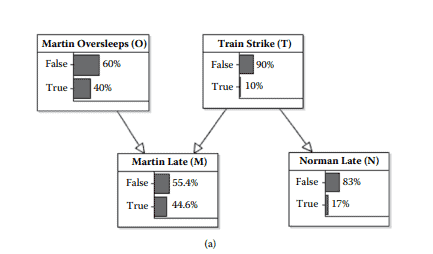
Norman is not the only person whose chances of being late increase when there is a train strike. Martin is also more likely to be late, but Martin depends less on trains than Norman and he is often late simply as a result of oversleeping. These additional factors can be modeled as shown in Figure 7.3.

You should add the new nodes and edges using AgenaRisk. We also need the probability tables for each of the nodes Martin oversleeps (Table 7.3) and Martin late (Table 7.4).

The table for node Martin late is more complicated than the table for Norman late because Martin late is conditioned on two nodes rather than one. Since each of the parent nodes has two states, true and false (we are still keeping the example as simple as possible), the number of combinations of parent states is four rather than two.

If you now run the model and display the probability graphs you should get the marginal probability values shown Figure 7.4(a). In particular, note that the marginal probability that Martin is late is equal to $0.446$ (i.e. $44.6 \%$ ). Box $7.1$ explains the underlying calculations involved in this.

But if we know that Norman is late, then the probability that Martin is late increases from the prior $0.446$ to $0.542$ as shown in Figure 7.4(b). Box $7.1$ explains the underlying calculations involved.

统计代写|贝叶斯分析代写Bayesian Analysis代考|Using Propagation to Make Special

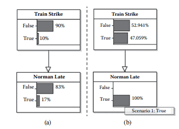
When we enter evidence and use it to update the probabilities in the way we have seen so far we call it propagation. In principle we can enter any number of observations anywhere in the BN model and use propagation to update the marginal probabilities of all the unobserved variables.
This can yield some exceptionally powerful types of analysis. For example, without showing the computational steps involved, if we first enter the observation that Martin is late we get the revised probabilities shown in Figure 7.5(a).

What the model is telling us here is that the most likely explanation for Martin’s lateness is Martin oversleeping; the revised probability of a train strike is still low. However, if we now discover that Norman is also late (Figure 7.5(b)) then Train strike (rather than Martin oversleeps) becomes the most likely explanation for Martin being late. This particular type of (backward) inference is called explaining away (or sometimes called nonmonotonic reasoning). Classical statistical tools alone do not enable this type of reasoning and what-if analysis.

In fact, as even the earlier simple example shows, BNs offer the following benefits:

  • Explicitly model causal factors – It is important to understand that this key benefit is in stark contrast to classical statistics whereby prediction models are normally developed by purely data-driven approaches. For example, the regression models introduced in Chapter 2 use historical data alone to produce equations relating dependent and independent variables. Such approaches not only fail to incorporate expert judgment in scenarios where there is insufficient data, but also fail to accommodate causal explanations. We will explore this further in Chapter $9 .$
  • Reason from effect to cause and vice versa-A BN will update the probability distributions for every unknown variable whenever an observation is entered into any node. So entering an observation in an “effect” node will result in back propagation, that is, revised probability distributions for the “cause” nodes and vice versa. Such backward reasoning of uncertainty is not possible in other approaches.
  • Reduce the burden of parameter acquisition-A BN will require fewer probability values and parameters than a full joint probability model. This modularity and compactness means that elicitation of probabilities is easier and explaining model results is made simpler.
统计代写|贝叶斯分析代写Bayesian Analysis代考|MAST90125

贝叶斯分析代考

统计代写|贝叶斯分析代写Bayesian Analysis代考|Accounting for Multiple Causes

诺曼并不是唯一一个在火车罢工时迟到的机会增加的人。马丁也更有可能迟到,但马丁比诺曼更少依赖火车,而且他经常因为睡过头而迟到。这些附加因素可以建模,如图 7.3 所示。

您应该使用 AgenaRisk 添加新节点和边。我们还需要每个节点 Martin oversleeps(表 7.3)和 Martin Late(表 7.4)的概率表。

节点 Martin Late 的表比 Norman Late 的表更复杂,因为 Martin Late 的条件是两个节点而不是一个节点。由于每个父节点都有两个状态,真和假(我们仍然使示例尽可能简单),父状态的组合数量是四个而不是两个。

如果你现在运行模型并显示概率图,你应该得到如图 7.4(a) 所示的边际概率值。特别注意,马丁迟到的边际概率等于0.446(IE44.6%)。盒子7.1解释了其中涉及的基础计算。

但是如果我们知道 Norman 迟到了,那么 Martin 迟到的概率会比之前的增加0.446至0.542如图 7.4(b) 所示。盒子7.1解释所涉及的基础计算。

统计代写|贝叶斯分析代写Bayesian Analysis代考|Using Propagation to Make Special

当我们输入证据并使用它以我们目前看到的方式更新概率时,我们称之为传播。原则上,我们可以在 BN 模型的任何位置输入任意数量的观测值,并使用传播来更新所有未观测变量的边际概率。
这可以产生一些异常强大的分析类型。例如,在不显示所涉及的计算步骤的情况下,如果我们首先输入 Martin 迟到的观察结果,我们会得到图 7.5(a) 所示的修正概率。

模型在这里告诉我们的是,马丁迟到最可能的解释是马丁睡过头了。修正后的火车罢工概率仍然很低。然而,如果我们现在发现 Norman 也迟到了(图 7.5(b)),那么火车罢工(而不是 Martin 睡过头)成为 Martin 迟到的最可能的解释。这种特殊类型的(反向)推理称为解释(或有时称为非单调推理)。单独的经典统计工具无法实现这种类型的推理和假设分析。

事实上,正如前面的简单示例所示,BN 提供了以下好处:

  • 显式建模因果因素——重要的是要了解,这一关键优势与经典统计形成鲜明对比,经典统计通常通过纯粹的数据驱动方法开发预测模型。例如,第 2 章介绍的回归模型仅使用历史数据来生成与因变量和自变量相关的方程。这种方法不仅无法在数据不足的情况下纳入专家判断,而且无法适应因果解释。我们将在本章中进一步探讨9.
  • 从结果到原因的原因,反之亦然 – 每当将观察输入任何节点时,BN 都会更新每个未知变量的概率分布。因此,在“影响”节点中输入观察结果将导致反向传播,即修改“原因”节点的概率分布,反之亦然。这种对不确定性的反向推理在其他方法中是不可能的。
  • 减少参数获取的负担——与完整的联合概率模型相比,BN 将需要更少的概率值和参数。这种模块化和紧凑性意味着概率的引出更容易,模型结果的解释也变得更简单。
统计代写|贝叶斯分析代写Bayesian Analysis代考 请认准statistics-lab™

统计代写请认准statistics-lab™. statistics-lab™为您的留学生涯保驾护航。

金融工程代写

金融工程是使用数学技术来解决金融问题。金融工程使用计算机科学、统计学、经济学和应用数学领域的工具和知识来解决当前的金融问题,以及设计新的和创新的金融产品。

非参数统计代写

非参数统计指的是一种统计方法,其中不假设数据来自于由少数参数决定的规定模型;这种模型的例子包括正态分布模型和线性回归模型。

广义线性模型代考

广义线性模型(GLM)归属统计学领域,是一种应用灵活的线性回归模型。该模型允许因变量的偏差分布有除了正态分布之外的其它分布。

术语 广义线性模型(GLM)通常是指给定连续和/或分类预测因素的连续响应变量的常规线性回归模型。它包括多元线性回归,以及方差分析和方差分析(仅含固定效应)。

有限元方法代写

有限元方法(FEM)是一种流行的方法,用于数值解决工程和数学建模中出现的微分方程。典型的问题领域包括结构分析、传热、流体流动、质量运输和电磁势等传统领域。

有限元是一种通用的数值方法,用于解决两个或三个空间变量的偏微分方程(即一些边界值问题)。为了解决一个问题,有限元将一个大系统细分为更小、更简单的部分,称为有限元。这是通过在空间维度上的特定空间离散化来实现的,它是通过构建对象的网格来实现的:用于求解的数值域,它有有限数量的点。边界值问题的有限元方法表述最终导致一个代数方程组。该方法在域上对未知函数进行逼近。[1] 然后将模拟这些有限元的简单方程组合成一个更大的方程系统,以模拟整个问题。然后,有限元通过变化微积分使相关的误差函数最小化来逼近一个解决方案。

tatistics-lab作为专业的留学生服务机构,多年来已为美国、英国、加拿大、澳洲等留学热门地的学生提供专业的学术服务,包括但不限于Essay代写,Assignment代写,Dissertation代写,Report代写,小组作业代写,Proposal代写,Paper代写,Presentation代写,计算机作业代写,论文修改和润色,网课代做,exam代考等等。写作范围涵盖高中,本科,研究生等海外留学全阶段,辐射金融,经济学,会计学,审计学,管理学等全球99%专业科目。写作团队既有专业英语母语作者,也有海外名校硕博留学生,每位写作老师都拥有过硬的语言能力,专业的学科背景和学术写作经验。我们承诺100%原创,100%专业,100%准时,100%满意。

随机分析代写


随机微积分是数学的一个分支,对随机过程进行操作。它允许为随机过程的积分定义一个关于随机过程的一致的积分理论。这个领域是由日本数学家伊藤清在第二次世界大战期间创建并开始的。

时间序列分析代写

随机过程,是依赖于参数的一组随机变量的全体,参数通常是时间。 随机变量是随机现象的数量表现,其时间序列是一组按照时间发生先后顺序进行排列的数据点序列。通常一组时间序列的时间间隔为一恒定值(如1秒,5分钟,12小时,7天,1年),因此时间序列可以作为离散时间数据进行分析处理。研究时间序列数据的意义在于现实中,往往需要研究某个事物其随时间发展变化的规律。这就需要通过研究该事物过去发展的历史记录,以得到其自身发展的规律。

回归分析代写

多元回归分析渐进(Multiple Regression Analysis Asymptotics)属于计量经济学领域,主要是一种数学上的统计分析方法,可以分析复杂情况下各影响因素的数学关系,在自然科学、社会和经济学等多个领域内应用广泛。

MATLAB代写

MATLAB 是一种用于技术计算的高性能语言。它将计算、可视化和编程集成在一个易于使用的环境中,其中问题和解决方案以熟悉的数学符号表示。典型用途包括:数学和计算算法开发建模、仿真和原型制作数据分析、探索和可视化科学和工程图形应用程序开发,包括图形用户界面构建MATLAB 是一个交互式系统,其基本数据元素是一个不需要维度的数组。这使您可以解决许多技术计算问题,尤其是那些具有矩阵和向量公式的问题,而只需用 C 或 Fortran 等标量非交互式语言编写程序所需的时间的一小部分。MATLAB 名称代表矩阵实验室。MATLAB 最初的编写目的是提供对由 LINPACK 和 EISPACK 项目开发的矩阵软件的轻松访问,这两个项目共同代表了矩阵计算软件的最新技术。MATLAB 经过多年的发展,得到了许多用户的投入。在大学环境中,它是数学、工程和科学入门和高级课程的标准教学工具。在工业领域,MATLAB 是高效研究、开发和分析的首选工具。MATLAB 具有一系列称为工具箱的特定于应用程序的解决方案。对于大多数 MATLAB 用户来说非常重要,工具箱允许您学习应用专业技术。工具箱是 MATLAB 函数(M 文件)的综合集合,可扩展 MATLAB 环境以解决特定类别的问题。可用工具箱的领域包括信号处理、控制系统、神经网络、模糊逻辑、小波、仿真等。

R语言代写问卷设计与分析代写
PYTHON代写回归分析与线性模型代写
MATLAB代写方差分析与试验设计代写
STATA代写机器学习/统计学习代写
SPSS代写计量经济学代写
EVIEWS代写时间序列分析代写
EXCEL代写深度学习代写
SQL代写各种数据建模与可视化代写

统计代写|贝叶斯分析代写Bayesian Analysis代考|STATS3023

如果你也在 怎样代写贝叶斯分析Bayesian Analysis这个学科遇到相关的难题,请随时右上角联系我们的24/7代写客服。

贝叶斯分析,一种统计推断方法(以英国数学家托马斯-贝叶斯命名),允许人们将关于人口参数的先验信息与样本所含信息的证据相结合,以指导统计推断过程。

statistics-lab™ 为您的留学生涯保驾护航 在代写贝叶斯分析Bayesian Analysis方面已经树立了自己的口碑, 保证靠谱, 高质且原创的统计Statistics代写服务。我们的专家在代写贝叶斯分析Bayesian Analysis代写方面经验极为丰富,各种代写贝叶斯分析Bayesian Analysis相关的作业也就用不着说。

我们提供的贝叶斯分析Bayesian Analysis及其相关学科的代写,服务范围广, 其中包括但不限于:

  • Statistical Inference 统计推断
  • Statistical Computing 统计计算
  • Advanced Probability Theory 高等概率论
  • Advanced Mathematical Statistics 高等数理统计学
  • (Generalized) Linear Models 广义线性模型
  • Statistical Machine Learning 统计机器学习
  • Longitudinal Data Analysis 纵向数据分析
  • Foundations of Data Science 数据科学基础
统计代写|贝叶斯分析代写Bayesian Analysis代考|STATS3023

统计代写|贝叶斯分析代写Bayesian Analysis代考|Second-Order Probability

Recall the Honest Joe’s and Shady Sam’s example we encountered in Chapter 4 (Box 4.7). In that example we expressed a belief in the chance of the die being fair or not, as a probability, while being aware that the fairness is also expressed as a probability. At first glance this looks very odd indeed since it suggests we are measuring a “probability about a probability.” We call this a second-order probability. If we think of the fairness of the die, and its chance of landing face up on a 6 , as a property of the die and how it is thrown, then we are expressing a degree of belief in the chance of the die having a given value. This is no different from expressing a degree of belief in a child reaching a given height when they mature in the sense that height and chance are both unknown properties of a thing that is of interest to us.
Example $6.10$ shows how we might model such second-order probabilities in practice.

Let us assume someone has smuggled a die out of either Shady Sam’s or Honest Joe’s, but we do not know which casino it has come from. We wish to determine the source of the die from (a) a prior belief about where the die is from and (b) data gained from rolling the die a number of times.

We have two alternative hypotheses we wish to test: Joe (“die comes from Honest Joe’s”) and Sam (“die comes from Shady Sam’s”). The respective prior probabilities for these hypotheses are:
$$
P(\text { Joe })=0.7 \quad P(\text { Sam })=0.3
$$
This is justified by the suspicion that our smuggler may be deterred by the extra personal risk in smuggling a die from Shady Sam’s compared with Honest Joe’s.

The data consists of 20 rolls of the die, observing there was one “6” and nineteen “not 6 ” results. So, we need to compute the likelihoods $\mathrm{P}($ Joe I data) and $\mathrm{P}($ Sam I data) and combine these (by Bayes theorem) with our prior beliefs about the hypotheses to get our posterior beliefs. To compute the likelihoods, recall that we believed that a die from Honest Joe’s was fair, with a chance of a 6, $p=1 / 6$, and from Shady Sam’s it was unfair, say, $p=1 / 12$. We can use these assumptions with the Binomial distribution to generate the likelihoods we need for the data, $X$ successes in 20 trials, given each of our hypotheses:
$$
P(X=x \mid p, 20)=\left(\begin{array}{l}
20 \
x
\end{array}\right) p^x(1-p)^{20-x}
$$
The results are shown in Table 6.4. Notice that we are expressing beliefs in hypotheses that are equivalent to beliefs about probabilities, in this case
$$
P(\text { Joe })=P(p=1 / 6)
$$
and
$$
P(\text { Sam })=P(p=1 / 12)
$$
From Table $6.4$ we can see that we now should favor the hypothesis that the die was sourced from Shady Sam’s rather than Honest Joe’s. This conclusion reverses our prior assumption (which had favored Honest Joe’s).

统计代写|贝叶斯分析代写Bayesian Analysis代考|A Very Simple Risk Assessment Problem

Since it is important for Norman to arrive on time for work, a number of people (including Norman himself) are interested in the probability that he will be late. Since Norman usually travels to work by train, one of the possible causes for Norman being late is a train strike. Because it is quite natural to reason from cause to effect we examine the relationship between a possible train strike and Norman being late. This relationship is represented by the causal model shown in Figure $7.1$ where the edge connects two nodes representing the variables “Train strike” $(T)$ to “Norman late” $(N)$.

It is obviously important that there is an edge between these variables since $T$ and $N$ are not independent (using the language of Chapter 5); common sense dictates that if there is a train strike then, assuming we know Norman travels by train, this will affect his ability to arrive on time. Common sense also determines the direction of the link since train strike causes Norman’s lateness rather than vice versa.

To ensure the example is as simple as possible we assume that both variables are discrete, having just two possible states: true and false.
Let us assume the following prior probability information:

  1. The probability of a train strike is $0.1$ (and therefore the probability of no train strike is 0.9). This information might be based on some subjective judgment given the most recent news or it might be based on the recent frequency of train strikes (i.e. one occurring about every 10 days). So the prior probability distribution for the variable “Train strike” is as shown in Table 7.1.
  2. The probability Norman is late given that there is a train strike is $0.8$ (and therefore the probability Norman is not late given that there is a train strike is $0.2$ ). The probability Norman is late given that there is not a train strike is $0.1$ (and therefore the probability Norman is not late given that there is not a train strike is 0.9). So, the (conditional) probability distribution for “Norman late” given “Train strike” is as shown in Table $7.2$.
统计代写|贝叶斯分析代写Bayesian Analysis代考|STATS3023

贝叶斯分析代考

统计代写|贝叶斯分析代写Bayesian Analysis代考|Second-Order Probability

回想一下我们在第 4 章中遇到的 Honest Joe 和 Shady Sam 的例子(方框 4.7) 。在该示例中,我们将相信骰子 是否公平的可能性表示为概率,同时意识到公平性也表示为概率。乍一看,这确实看起来很奇怪,因为它表明我 们正在测量“概率的概率”。我们称之为二阶概率。如果我们将骰子的公平性,以及它正面朝上落在 6 的机会视为 骰子的属性以及它是如何抛出的,那么我们就表达了对骰子具有给定概率的信念的程度。价值。这与在孩子成熟 时表达某种程度的信念没有什么不同,因为身高和机会都是我们感兴趣的事物的末知属性。 例子6.10展示了我们如何在实践中模拟这种二阶概率。
让我们假设有人从 Shady Sam’s 或 Honest Joe’s 走私了一个骰子,但我们不知道它来自哪个赌场。我们希望从 (a) 关于骰子来自哪里的先验信念和(b)通过多次滚动骰子获得的数据来确定骰子的来源。
我们有两个我们希望测试的替代假设: Joe (“死来自 Honest Joe’s”) 和 Sam (“死来自 Shady Sam’s”) 。这些假 设各自的先验概率是:
$$
P(\text { Joe })=0.7 \quad P(\text { Sam })=0.3
$$
这是有道理的,因为我们的走私者可能会因为从 Shady Sam’s 走私模具与 Honest Joe’s 相比额外的个人风险而被吓倒。
数据由 20 卷模具组成,观察到有 1 个“ 6 “和 19 个“非 $6^{\prime \prime}$ 结果。所以,我们需要计算可能性 $\mathrm{P}$ (乔一世数据) 和 $\mathrm{P}($ Sam I 数据) 并将这些 (通过贝叶斯定理) 与我们对假设的先前信念相结合,以获得我们的后验信念。要计算可 能性,请回想一下,我们认为 Honest Joe 的骰子是公平的,有 6 的机会, $p=1 / 6$ ,从 Shady Sam 那里说,这 是不公平的, $p=1 / 12$. 我们可以将这些假设与二项分布一起使用来生成数据所需的可能性, $X$ 根据我们的每个 假设,在 20 次试验中取得了成功:
$$
P(X=x \mid p, 20)=(20 x) p^x(1-p)^{20-x}
$$
结果如表 $6.4$ 所示。请注意,在这种情况下,我们表达的假设信念等同于概率信念
$$
P(\text { Joe })=P(p=1 / 6)
$$

$$
P(\mathrm{Sam})=P(p=1 / 12)
$$
从表6.4我们可以看到,我们现在应该支持骰子来自 Shady Sam 而不是 Honest Joe 的假设。这个结论推翻了我 们之前的假设(这有利于诚实乔的假设)。

统计代写|贝叶斯分析代写Bayesian Analysis代考|A Very Simple Risk Assessment Problem

由于 Norman 准时上班很重要,因此许多人(包括 Norman 本人)对他迟到的概率感兴趣。由于诺曼通常乘火车上班,因此诺曼迟到的可能原因之一是火车罢工。因为从因果推理是很自然的,所以我们研究了可能的火车罢工与诺曼迟到之间的关系。这种关系由图 1 所示的因果模型表示7.1其中边连接代表变量“火车罢工”的两个节点(吨)到“诺曼迟到”(ñ).

这些变量之间存在优势显然很重要,因为吨和ñ不是独立的(使用第 5 章的语言);常识表明,如果发生火车罢工,假设我们知道诺曼乘火车旅行,这将影响他准时到达的能力。常识也决定了链接的方向,因为火车撞击导致诺曼迟到,而不是相反。

为了确保示例尽可能简单,我们假设两个变量都是离散的,只有两种可能的状态:真和假。
让我们假设以下先验概率信息:

  1. 火车撞车的概率是0.1(因此没有火车撞击的概率是 0.9)。该信息可能基于给定最新消息的一些主观判断,也可能基于最近的火车罢工频率(即大约每 10 天发生一次)。因此,变量“火车罢工”的先验概率分布如表 7.1 所示。
  2. 鉴于火车罢工,诺曼迟到的概率是0.8(因此,鉴于火车罢工,诺曼不迟到的概率是0.2)。鉴于没有火车罢工,诺曼迟到的概率是0.1(因此,鉴于没有火车罢工,诺曼不迟到的概率是 0.9)。因此,给定“火车罢工”的“诺曼晚点”的(条件)概率分布如表所示7.2.
统计代写|贝叶斯分析代写Bayesian Analysis代考 请认准statistics-lab™

统计代写请认准statistics-lab™. statistics-lab™为您的留学生涯保驾护航。

金融工程代写

金融工程是使用数学技术来解决金融问题。金融工程使用计算机科学、统计学、经济学和应用数学领域的工具和知识来解决当前的金融问题,以及设计新的和创新的金融产品。

非参数统计代写

非参数统计指的是一种统计方法,其中不假设数据来自于由少数参数决定的规定模型;这种模型的例子包括正态分布模型和线性回归模型。

广义线性模型代考

广义线性模型(GLM)归属统计学领域,是一种应用灵活的线性回归模型。该模型允许因变量的偏差分布有除了正态分布之外的其它分布。

术语 广义线性模型(GLM)通常是指给定连续和/或分类预测因素的连续响应变量的常规线性回归模型。它包括多元线性回归,以及方差分析和方差分析(仅含固定效应)。

有限元方法代写

有限元方法(FEM)是一种流行的方法,用于数值解决工程和数学建模中出现的微分方程。典型的问题领域包括结构分析、传热、流体流动、质量运输和电磁势等传统领域。

有限元是一种通用的数值方法,用于解决两个或三个空间变量的偏微分方程(即一些边界值问题)。为了解决一个问题,有限元将一个大系统细分为更小、更简单的部分,称为有限元。这是通过在空间维度上的特定空间离散化来实现的,它是通过构建对象的网格来实现的:用于求解的数值域,它有有限数量的点。边界值问题的有限元方法表述最终导致一个代数方程组。该方法在域上对未知函数进行逼近。[1] 然后将模拟这些有限元的简单方程组合成一个更大的方程系统,以模拟整个问题。然后,有限元通过变化微积分使相关的误差函数最小化来逼近一个解决方案。

tatistics-lab作为专业的留学生服务机构,多年来已为美国、英国、加拿大、澳洲等留学热门地的学生提供专业的学术服务,包括但不限于Essay代写,Assignment代写,Dissertation代写,Report代写,小组作业代写,Proposal代写,Paper代写,Presentation代写,计算机作业代写,论文修改和润色,网课代做,exam代考等等。写作范围涵盖高中,本科,研究生等海外留学全阶段,辐射金融,经济学,会计学,审计学,管理学等全球99%专业科目。写作团队既有专业英语母语作者,也有海外名校硕博留学生,每位写作老师都拥有过硬的语言能力,专业的学科背景和学术写作经验。我们承诺100%原创,100%专业,100%准时,100%满意。

随机分析代写


随机微积分是数学的一个分支,对随机过程进行操作。它允许为随机过程的积分定义一个关于随机过程的一致的积分理论。这个领域是由日本数学家伊藤清在第二次世界大战期间创建并开始的。

时间序列分析代写

随机过程,是依赖于参数的一组随机变量的全体,参数通常是时间。 随机变量是随机现象的数量表现,其时间序列是一组按照时间发生先后顺序进行排列的数据点序列。通常一组时间序列的时间间隔为一恒定值(如1秒,5分钟,12小时,7天,1年),因此时间序列可以作为离散时间数据进行分析处理。研究时间序列数据的意义在于现实中,往往需要研究某个事物其随时间发展变化的规律。这就需要通过研究该事物过去发展的历史记录,以得到其自身发展的规律。

回归分析代写

多元回归分析渐进(Multiple Regression Analysis Asymptotics)属于计量经济学领域,主要是一种数学上的统计分析方法,可以分析复杂情况下各影响因素的数学关系,在自然科学、社会和经济学等多个领域内应用广泛。

MATLAB代写

MATLAB 是一种用于技术计算的高性能语言。它将计算、可视化和编程集成在一个易于使用的环境中,其中问题和解决方案以熟悉的数学符号表示。典型用途包括:数学和计算算法开发建模、仿真和原型制作数据分析、探索和可视化科学和工程图形应用程序开发,包括图形用户界面构建MATLAB 是一个交互式系统,其基本数据元素是一个不需要维度的数组。这使您可以解决许多技术计算问题,尤其是那些具有矩阵和向量公式的问题,而只需用 C 或 Fortran 等标量非交互式语言编写程序所需的时间的一小部分。MATLAB 名称代表矩阵实验室。MATLAB 最初的编写目的是提供对由 LINPACK 和 EISPACK 项目开发的矩阵软件的轻松访问,这两个项目共同代表了矩阵计算软件的最新技术。MATLAB 经过多年的发展,得到了许多用户的投入。在大学环境中,它是数学、工程和科学入门和高级课程的标准教学工具。在工业领域,MATLAB 是高效研究、开发和分析的首选工具。MATLAB 具有一系列称为工具箱的特定于应用程序的解决方案。对于大多数 MATLAB 用户来说非常重要,工具箱允许您学习应用专业技术。工具箱是 MATLAB 函数(M 文件)的综合集合,可扩展 MATLAB 环境以解决特定类别的问题。可用工具箱的领域包括信号处理、控制系统、神经网络、模糊逻辑、小波、仿真等。

R语言代写问卷设计与分析代写
PYTHON代写回归分析与线性模型代写
MATLAB代写方差分析与试验设计代写
STATA代写机器学习/统计学习代写
SPSS代写计量经济学代写
EVIEWS代写时间序列分析代写
EXCEL代写深度学习代写
SQL代写各种数据建模与可视化代写

金融代写|风险理论代写Risk theory代考|MATH4128

如果你也在 怎样代写风险理论Risk theory这个学科遇到相关的难题,请随时右上角联系我们的24/7代写客服。

风险理论试图解释人们在面对未来的不确定性时做出的决定。通常情况下,可以应用风险理论的情况涉及世界的一些可能状态,一些可能的决定,以及每种状态和决定的组合的结果。

statistics-lab™ 为您的留学生涯保驾护航 在代写风险理论Risk theory方面已经树立了自己的口碑, 保证靠谱, 高质且原创的统计Statistics代写服务。我们的专家在代写风险理论Risk theory相关的作业也就用不着说。

我们提供的风险理论Risk theory及其相关学科的代写,服务范围广, 其中包括但不限于:

  • Statistical Inference 统计推断
  • Statistical Computing 统计计算
  • Advanced Probability Theory 高等楖率论
  • Advanced Mathematical Statistics 高等数理统计学
  • (Generalized) Linear Models 广义线性模型
  • Statistical Machine Learning 统计机器学习
  • Longitudinal Data Analysis 纵向数据分析
  • Foundations of Data Science 数据科学基础
金融代写|风险理论代写Risk theory代考|MATH4128

金融代写|风险理论代写Risk theory代考|Bayes and Empirical Bayes

Let $\boldsymbol{X}=\left(X_1, \ldots, X_n\right)$ be a vector of r.v.s describing the outcome of a statistical experiment. For example, in the insurance context, $n$ can be the number of persons insured for losses due to accidents in the previous year, and $X_i$ the payment made to the $i$ th.

A traditional (frequentists’) model is to assume the $X_i$ to be i.i.d. with a common distribution $F_\theta$ where $\theta$ is an unknown parameter (possibly multidimensional). F.g. in the accident insurance example, one could let $b$ denote the probability that a person has an accident within one year, $b=\mathbb{P}\left(X_i>0\right)$, and one could assume that the cost of the accident has a $\operatorname{gamma}(\alpha, \lambda)$ distribution. Thus the density of $X_i$ is
$$
f_{b, \alpha, \lambda}(x)=b \mathbb{1}{x=0}+(1-b) \frac{\lambda^\alpha x^{\alpha-1}}{\Gamma(\alpha)} \mathrm{e}^{-\lambda x_1} \mathbb{1}{x>0}
$$
w.r.t. the measure defined as Lebesgue measure $\mathrm{d} x$ on $(0, \infty)$ with an added atom of unit size at $x=0$. Then $\theta=(b, \alpha, \lambda)$, and the conventional statistical procedure would be to compute estimates $\widehat{b}, \widehat{\alpha}, \widehat{\lambda}$ of $b, \alpha, \lambda$. These estimates could then be used as basis for computing first the expectation
$$
\mathbb{E}{\widehat{\theta}} X=\mathbb{E}{\widehat{b}, \widehat{\alpha}, \widehat{\lambda}} X=(1-\widehat{b}) \widehat{\alpha} / \widehat{\lambda}
$$
of $X$ under the estimated parameters, and next one could use $\mathbb{E}_{\widehat{\theta}} X$ as the net premium and add a loading corresponding to one of the premium rules discussed in Sect. I.3. For example, the expected value principle would lead to the premium
$$
p=(1+\eta)(1-\widehat{b}) \widehat{\alpha} / \widehat{\lambda}
$$

金融代写|风险理论代写Risk theory代考|The Bayes Premium

We now turn to the general implementation of Bayesian ideas in insurance. Here one considers an insured with risk parameter $Z^1$ and an r.v. with distribution $\pi^{(0)}(\cdot)$, with observable past claims $X_1, \ldots, X_n$ and an unobservable claim amount $X_{n+1}$ for year $n+1$. The aim is to assert which (net) premium the insured is to pay in year $n+1$

For a fixed $\zeta$, let $\mu(\zeta)=\mathbb{E}\zeta X{n+1}$, where $\mathbb{E}\zeta[\cdot]=\mathbb{E}[\cdot \mid Z=\zeta]$. The (net) collective premium $H{\mathrm{Coll}}$ is $\mathbb{E} \mu(\boldsymbol{Z})=\mathbb{E} X_{n+1}$. This is the premium we would charge without prior statistics $X_1, \ldots, X_n$ on the insured. The individual premium is $H_{\text {Ind }}=\mathbb{E}\left[X_{n+1} \mid \boldsymbol{Z}\right]=\mu(\boldsymbol{Z})$. This is the ideal net premium in the sense of supplying the complete relevant prior information on the customer. The Bayes premium $H_{\text {Bayes }}$ is defined as $\mathbb{E}\left[\mu(\boldsymbol{Z}) \mid X_1, \ldots, X_n\right]$. That is, $H_{\text {Bayes }}$ is the expected value of $X_{n+1}$ in the posterior distribution.

Note that the individual premium is unobservable because $\boldsymbol{Z}$ is so; the Bayes premium is ‘our best guess of $H_{\text {Ind }}$ based upon the observations’. To make this precise, let $H^$ be another premium rule, that is, a function of $X_1, \ldots, X_n$ and the prior parameters. We then define its loss as $$ \ell_{H^}=\mathbb{E}\left[\mu(\boldsymbol{Z})-H^\right]^2=\left|\mu(\boldsymbol{Z})-H^\right|^2
$$
where $|X|=\left(\mathbb{E} X^2\right)^{1 / 2}$ is the $L_2$-norm (in obvious notation, we write $\ell_{\text {Coll }}=\ell_{H_{\text {Coll }}}$ etc). In mathematical terms, the optimality property of the Bayes premium is then that it minimizes the quadratic loss:
Theorem 1.3 For any $H^, \ell_{\text {Bayes }} \leq \ell_{H^}$. That is,
$$
\mathbb{E}\left(H_{\text {Bayes }}-H_{\text {Ind }}\right)^2 \leq \mathbb{E}\left(H^*-H_{\text {Ind }}\right)^2
$$

金融代写|风险理论代写Risk theory代考|MATH4128

风险理论代考

金融代写|风险理论代写Risk theory代考|Bayes and Empirical Bayes

让 $\boldsymbol{X}=\left(X_1, \ldots, X_n\right)$ 是描述统计实验结果的 rvs 向量。例如,在保险方面, $n$ 可以是上一年因事故损失的投保 人数,以及 $X_i$ 支付给 $i$ th。
传统的 (常客) 模型是假设 $X_i$ 具有共同分布的独立同分布 $F_\theta$ 在哪里 $\theta$ 是一个末知参数 (可能是多维的)。 $F g$ 在意 外保险的例子中,可以让 $b$ 表示一个人在一年内发生事故的概率, $b=\mathbb{P}\left(X_i>0\right)$ ,并且可以假设事故的成本有 $\operatorname{gamma}(\alpha, \lambda)$ 分配。因此密度 $X_i$ 是
$$
f_{b, \alpha, \lambda}(x)=b 1 x=0+(1-b) \frac{\lambda^\alpha x^{\alpha-1}}{\Gamma(\alpha)} \mathrm{e}^{-\lambda x_1} 1 x>0
$$
wrt 定义为 Lebesgue 度量的度量 $\mathrm{d} x$ 上 $(0, \infty)$ 添加一个单位大小的原子 $x=0$. 然后 $\theta=(b, \alpha, \lambda)$ ,而传统的统 计程序是计算估计值 $\hat{b}, \widehat{\alpha}, \widehat{\lambda}$ 的 $b, \alpha, \lambda$. 然后可以将这些估计值用作首先计算期望值的基础
$$
\mathbb{E} \hat{\theta} X=\mathbb{E} \hat{b}, \widehat{\alpha}, \hat{\lambda} X=(1-\hat{b}) \widehat{\alpha} / \widehat{\lambda}
$$
的 $X$ 在估计的参数下,下一个可以使用 $\mathbb{E}_{\hat{\theta}} X$ 作为净溢价,并添加与第 3 节中讨论的溢价规则之一相对应的负载。 -.3。例如,期望值原则会导致溢价
$$
p=(1+\eta)(1-\hat{b}) \widehat{\alpha} / \widehat{\lambda}
$$

金融代写|风险理论代写Risk theory代考|The Bayes Premium

我们现在转向保险业中贝叶斯思想的一般实施。这里考虑一个具有风险参数的被保险人 $Z^1$ 和一个有分布的房车 $\pi^{(0)}(\cdot)$ ,具有可观察到的过去声明 $X_1, \ldots, X_n$ 和不可观察的索赔金额 $X_{n+1}$ 一年 $n+1$. 目的是确定被保险人将 在一年内支付的 (净) 保费 $n+1$
对于一个固定 $\zeta$ ,让 $\mu(\zeta)=\mathbb{E} \zeta X n+1$ ,在哪里 $\mathbb{E} \zeta[\cdot]=\mathbb{E}[\cdot \mid Z=\zeta]$. (净) 集体溢价 $H$ Coll是 $\mathbb{E} \mu(\boldsymbol{Z})=\mathbb{E} X_{n+1}$. 这是我们在没有事先统计的情况下收取的保费 $X_1, \ldots, X_n$ 在被保险人身上。个人保费为 $H_{\text {Ind }}=\mathbb{E}\left[X_{n+1} \mid \boldsymbol{Z}\right]=\mu(\boldsymbol{Z})$. 在提供有关客户的完整相关先验信息的意义上,这是理想的净溢价。贝叶斯
请注意,个人溢价是不可观察的,因为 $Z$ 是这样的;贝叶斯溢价是“我们最好的猜测 $H_{\text {Ind }}$ 根据观察”。为了使这一 点更精确,让 是另一个溢价规则,即 $X_1, \ldots, X_n$ 和先验参数。然后我们将其损失定义为
在哪里 $|X|=\left(\mathbb{E} X^2\right)^{1 / 2}$ 是个 $L_2$-norm (在明显的符号中,我们写 $\ell_{\text {Coll }}=\ell_{H_{\text {Coll }}}$ ETC) 。用数学术语来说, 贝叶斯溢价的最优性是它最小化二次损失:
$$
\mathbb{E}\left(H_{\text {Bayes }}-H_{\text {Ind }}\right)^2 \leq \mathbb{E}\left(H^*-H_{\text {Ind }}\right)^2
$$

金融代写|风险理论代写Risk theory代考 请认准statistics-lab™

统计代写请认准statistics-lab™. statistics-lab™为您的留学生涯保驾护航。统计代写|python代写代考

随机过程代考

在概率论概念中,随机过程随机变量的集合。 若一随机系统的样本点是随机函数,则称此函数为样本函数,这一随机系统全部样本函数的集合是一个随机过程。 实际应用中,样本函数的一般定义在时间域或者空间域。 随机过程的实例如股票和汇率的波动、语音信号、视频信号、体温的变化,随机运动如布朗运动、随机徘徊等等。

贝叶斯方法代考

贝叶斯统计概念及数据分析表示使用概率陈述回答有关未知参数的研究问题以及统计范式。后验分布包括关于参数的先验分布,和基于观测数据提供关于参数的信息似然模型。根据选择的先验分布和似然模型,后验分布可以解析或近似,例如,马尔科夫链蒙特卡罗 (MCMC) 方法之一。贝叶斯统计概念及数据分析使用后验分布来形成模型参数的各种摘要,包括点估计,如后验平均值、中位数、百分位数和称为可信区间的区间估计。此外,所有关于模型参数的统计检验都可以表示为基于估计后验分布的概率报表。

广义线性模型代考

广义线性模型(GLM)归属统计学领域,是一种应用灵活的线性回归模型。该模型允许因变量的偏差分布有除了正态分布之外的其它分布。

statistics-lab作为专业的留学生服务机构,多年来已为美国、英国、加拿大、澳洲等留学热门地的学生提供专业的学术服务,包括但不限于Essay代写,Assignment代写,Dissertation代写,Report代写,小组作业代写,Proposal代写,Paper代写,Presentation代写,计算机作业代写,论文修改和润色,网课代做,exam代考等等。写作范围涵盖高中,本科,研究生等海外留学全阶段,辐射金融,经济学,会计学,审计学,管理学等全球99%专业科目。写作团队既有专业英语母语作者,也有海外名校硕博留学生,每位写作老师都拥有过硬的语言能力,专业的学科背景和学术写作经验。我们承诺100%原创,100%专业,100%准时,100%满意。

机器学习代写

随着AI的大潮到来,Machine Learning逐渐成为一个新的学习热点。同时与传统CS相比,Machine Learning在其他领域也有着广泛的应用,因此这门学科成为不仅折磨CS专业同学的“小恶魔”,也是折磨生物、化学、统计等其他学科留学生的“大魔王”。学习Machine learning的一大绊脚石在于使用语言众多,跨学科范围广,所以学习起来尤其困难。但是不管你在学习Machine Learning时遇到任何难题,StudyGate专业导师团队都能为你轻松解决。

多元统计分析代考


基础数据: $N$ 个样本, $P$ 个变量数的单样本,组成的横列的数据表
变量定性: 分类和顺序;变量定量:数值
数学公式的角度分为: 因变量与自变量

时间序列分析代写

随机过程,是依赖于参数的一组随机变量的全体,参数通常是时间。 随机变量是随机现象的数量表现,其时间序列是一组按照时间发生先后顺序进行排列的数据点序列。通常一组时间序列的时间间隔为一恒定值(如1秒,5分钟,12小时,7天,1年),因此时间序列可以作为离散时间数据进行分析处理。研究时间序列数据的意义在于现实中,往往需要研究某个事物其随时间发展变化的规律。这就需要通过研究该事物过去发展的历史记录,以得到其自身发展的规律。

回归分析代写

多元回归分析渐进(Multiple Regression Analysis Asymptotics)属于计量经济学领域,主要是一种数学上的统计分析方法,可以分析复杂情况下各影响因素的数学关系,在自然科学、社会和经济学等多个领域内应用广泛。

MATLAB代写

MATLAB 是一种用于技术计算的高性能语言。它将计算、可视化和编程集成在一个易于使用的环境中,其中问题和解决方案以熟悉的数学符号表示。典型用途包括:数学和计算算法开发建模、仿真和原型制作数据分析、探索和可视化科学和工程图形应用程序开发,包括图形用户界面构建MATLAB 是一个交互式系统,其基本数据元素是一个不需要维度的数组。这使您可以解决许多技术计算问题,尤其是那些具有矩阵和向量公式的问题,而只需用 C 或 Fortran 等标量非交互式语言编写程序所需的时间的一小部分。MATLAB 名称代表矩阵实验室。MATLAB 最初的编写目的是提供对由 LINPACK 和 EISPACK 项目开发的矩阵软件的轻松访问,这两个项目共同代表了矩阵计算软件的最新技术。MATLAB 经过多年的发展,得到了许多用户的投入。在大学环境中,它是数学、工程和科学入门和高级课程的标准教学工具。在工业领域,MATLAB 是高效研究、开发和分析的首选工具。MATLAB 具有一系列称为工具箱的特定于应用程序的解决方案。对于大多数 MATLAB 用户来说非常重要,工具箱允许您学习应用专业技术。工具箱是 MATLAB 函数(M 文件)的综合集合,可扩展 MATLAB 环境以解决特定类别的问题。可用工具箱的领域包括信号处理、控制系统、神经网络、模糊逻辑、小波、仿真等。

R语言代写问卷设计与分析代写
PYTHON代写回归分析与线性模型代写
MATLAB代写方差分析与试验设计代写
STATA代写机器学习/统计学习代写
SPSS代写计量经济学代写
EVIEWS代写时间序列分析代写
EXCEL代写深度学习代写
SQL代写各种数据建模与可视化代写

金融代写|风险理论代写Risk theory代考|STAT4901

如果你也在 怎样代写风险理论Risk theory这个学科遇到相关的难题,请随时右上角联系我们的24/7代写客服。

风险理论试图解释人们在面对未来的不确定性时做出的决定。通常情况下,可以应用风险理论的情况涉及世界的一些可能状态,一些可能的决定,以及每种状态和决定的组合的结果。

statistics-lab™ 为您的留学生涯保驾护航 在代写风险理论Risk theory方面已经树立了自己的口碑, 保证靠谱, 高质且原创的统计Statistics代写服务。我们的专家在代写风险理论Risk theory相关的作业也就用不着说。

我们提供的风险理论Risk theory及其相关学科的代写,服务范围广, 其中包括但不限于:

  • Statistical Inference 统计推断
  • Statistical Computing 统计计算
  • Advanced Probability Theory 高等楖率论
  • Advanced Mathematical Statistics 高等数理统计学
  • (Generalized) Linear Models 广义线性模型
  • Statistical Machine Learning 统计机器学习
  • Longitudinal Data Analysis 纵向数据分析
  • Foundations of Data Science 数据科学基础
金融代写|风险理论代写Risk theory代考|STAT4901

金融代写|风险理论代写Risk theory代考|Reinsurance

Reinsurance means that the company (the cedent or first insurer) insures a part of the risk at another insurance company (the reinsurer). The purposes of reinsurance are to reduce risk and/or to reduce the risk volume of the company.

We start by formulating the basic concepts within the framework of a single risk $X \geq 0$. A reinsurance arrangement is then defined in terms of a function $r(x)$ with the property $0 \leq r(x) \leq x$. Here $r(x)$ is the amount of the claim $x$ to be paid by the reinsurer and $s(x)=x-r(x)$ the amount to be paid by the cedent. The function $s(x)$ is referred to as the retention function. The most common examples are the following two:

  • Proportional reinsurance $r(x)=(1-\theta) x, s(x)=\theta x$ for some $\theta \in(0,1)$. Also called quota share reinsurance.
  • Stop-loss reinsurance $r(x)=(x-b)^{+}$for some $b \in(0, \infty)$, referred to as the retention limit. The retention function is $x \wedge b$.

Concerning terminology, note that in the actuarial literature the stop-loss transform of $F(x)=\mathbb{P}(X \leq x)$ (or, equivalently, of $X)$ is defined as the function
$$
b \mapsto \mathbb{E}(X-b)^{+}=\int_b^{\infty}(x-b) F(\mathrm{~d} x)=\int_b^{\infty} \bar{F}(x) \mathrm{d} x
$$
(the last equality follows by integration by parts, see formula (A.1.1) in the Appendix). It shows up in a number of different contexts, see e.g. Sect. VIII.2.1, where some of its main properties are listed.

The risk $X$ is often the aggregate claims amount $A=\sum_1^N V_i$ in a certain line of business during one year; one then talks of global reinsurance. However, reinsurance may also be done locally, i.e. at the level of individual claims. Then, if $N$ is the number of claims during the period and $V_1, V_2, \ldots$ their sizes, then the amounts paid by reinsurer, resp. the cedent, are
$$
\sum_{i=1}^N r\left(V_i\right), \text { resp. } \sum_{i=1}^N s\left(V_i\right)
$$

金融代写|风险理论代写Risk theory代考|The Poisson Process

By a (simple) point process $\mathscr{N}$ on a set $\Omega \subseteq \mathbb{R}^d$ we understand a random collection of points in $\Omega$ [simple means that there are no multiple points]. We are almost exclusively concerned with the case $\Omega=[0, \infty)$. The point process can then be specified by the sequence $T_1, T_2, \ldots$ of interarrival times such that the points are $T_1, T_1+T_2, \ldots$ The associated counting process ${N(t)}_{t \geq 0}$ is defined by letting $N(t)$ be the number of points in $[0, t]$. Write
$$
\mathscr{N}(s, t]=N(t)-N(s)=#\left{n: s<T_1+\cdots+T_n \leq t\right}
$$
for the increment of ${N(t)}$ over $(s, t]$ or equivalently the number of points in $(s, t]$.
Definition 5.2 $\mathscr{N}$ is a Poisson process on $[0, \infty)$ with rate $\lambda$ if ${N(t)}$ has independent increments and $N(t)-N(s)$ has a Poisson $(\lambda(t-s))$ distribution for $s<t$.

Here independence of increments means independence of increments over disjoint intervals.

It is not difficult to extend the reasoning hehind example 1) ahnve to conclude. that for a large insurance portfolio, the number of claims in disjoint time intervals are independent Poisson r.v.s, and so the times of occurrences of claims form a Poisson process. There are, however, different ways to approach the Poisson process. In particular, the infinitesimal view in part (iii) of the following result will prove useful for many of our purposes.

金融代写|风险理论代写Risk theory代考|STAT4901

风险理论代考

金融代写|风险理论代写Risk theory代考|Reinsurance

再保险是指公司 (分出人或第一保险公司) 为另一家保险公司 (再保险公司) 投保部分风险。再保险的目的是降 低风险和/或降低公司的风险量。
我们首先在单一风险的框架内制定基本概念 $X \geq 0$. 然后根据功能定义再保险安排 $r(x)$ 与财产 $0 \leq r(x) \leq x$. 这 里 $r(x)$ 是索赔金额 $x$ 由再保险人支付,并且 $s(x)=x-r(x)$ 分出人须支付的款额。功能 $s(x)$ 称为保留函数。最 常见的例子有以下两个:

  • 比例再保险 $r(x)=(1-\theta) x, s(x)=\theta x$ 对于一些 $\theta \in(0,1)$. 也称为配额份额再保险。
  • 止损再保险 $r(x)=(x-b)^{+}$对于一些 $b \in(0, \infty)$ ,称为保留限制。保留函数为 $x \wedge b$.
    关于术语,请注意在精算文献中,止损变换 $F(x)=\mathbb{P}(X \leq x)$ (或者,等效地, $X$ )被定义为函数
    $$
    b \mapsto \mathbb{E}(X-b)^{+}=\int_b^{\infty}(x-b) F(\mathrm{~d} x)=\int_b^{\infty} \bar{F}(x) \mathrm{d} x
    $$
    (最后一个等式后面是分部积分,见附录中的公式 (A.1.1) )。它出现在许多不同的上下文中,例如参见 Sect。 VIII.2.1,其中列出了它的一些主要属性。
    风险 $X$ 通常是总索赔额 $A=\sum_1^N V_i$ 一年内从事某项业务;然后有人谈到全球再保险。然而,再保险也可以在当 地进行,即在个人索赔层面。那么,如果 $N$ 是该期间的索赔数量,并且 $V_1, V_2, \ldots$ 他们的规模,然后是再保险公 司支付的金额,resp。分出商是
    $$
    \sum_{i=1}^N r\left(V_i\right), \text { resp. } \sum_{i=1}^N s\left(V_i\right)
    $$

金融代写|风险理论代写Risk theory代考|The Poisson Process

通过 (简单) 点过程 $\mathscr{N}$ 在一组 $\Omega \subseteq \mathbb{R}^d$ 我们理解点的随机集合 $\Omega$ [简单意味着没有多个点]。我们几乎只关心这个 案子 $\Omega=[0, \infty)$. 然后可以通过序列指定点过程 $T_1, T_2, \ldots$ 到达间隔时间,使得点是 $T_1, T_1+T_2, \ldots$. 相关的计 数过程 $N(t)_{t \geq 0}$ 定义为 $N(t)$ 是点的数量 $[0, t]$. 写
对于增量 $N(t)$ 超过 $(s, t]$ 或等效的点数 $(s, t]$.
定义 5.2 $N$ 是一个泊松过程 $[0, \infty)$ 有率 $\lambda$ 如果 $N(t)$ 有独立的增量和 $N(t)-N(s)$ 有泊松 $(\lambda(t-s))$ 分配给 $s<t$
这里增量的独立性意味着增量在不相交的间隔上的独立性。
不难推导出例子 1) 后面的推理来得出结论。即对于大型保险组合,不相交时间间隔内的理赔次数是独立的
Poisson rvs,因此理赔发生的次数构成一个 Poisson 过程。然而,有不同的方法来处理泊松过程。特别是,以下 结果的 (iii) 部分中的无穷小视图将证明对我们的许多目的有用。

金融代写|风险理论代写Risk theory代考 请认准statistics-lab™

统计代写请认准statistics-lab™. statistics-lab™为您的留学生涯保驾护航。统计代写|python代写代考

随机过程代考

在概率论概念中,随机过程随机变量的集合。 若一随机系统的样本点是随机函数,则称此函数为样本函数,这一随机系统全部样本函数的集合是一个随机过程。 实际应用中,样本函数的一般定义在时间域或者空间域。 随机过程的实例如股票和汇率的波动、语音信号、视频信号、体温的变化,随机运动如布朗运动、随机徘徊等等。

贝叶斯方法代考

贝叶斯统计概念及数据分析表示使用概率陈述回答有关未知参数的研究问题以及统计范式。后验分布包括关于参数的先验分布,和基于观测数据提供关于参数的信息似然模型。根据选择的先验分布和似然模型,后验分布可以解析或近似,例如,马尔科夫链蒙特卡罗 (MCMC) 方法之一。贝叶斯统计概念及数据分析使用后验分布来形成模型参数的各种摘要,包括点估计,如后验平均值、中位数、百分位数和称为可信区间的区间估计。此外,所有关于模型参数的统计检验都可以表示为基于估计后验分布的概率报表。

广义线性模型代考

广义线性模型(GLM)归属统计学领域,是一种应用灵活的线性回归模型。该模型允许因变量的偏差分布有除了正态分布之外的其它分布。

statistics-lab作为专业的留学生服务机构,多年来已为美国、英国、加拿大、澳洲等留学热门地的学生提供专业的学术服务,包括但不限于Essay代写,Assignment代写,Dissertation代写,Report代写,小组作业代写,Proposal代写,Paper代写,Presentation代写,计算机作业代写,论文修改和润色,网课代做,exam代考等等。写作范围涵盖高中,本科,研究生等海外留学全阶段,辐射金融,经济学,会计学,审计学,管理学等全球99%专业科目。写作团队既有专业英语母语作者,也有海外名校硕博留学生,每位写作老师都拥有过硬的语言能力,专业的学科背景和学术写作经验。我们承诺100%原创,100%专业,100%准时,100%满意。

机器学习代写

随着AI的大潮到来,Machine Learning逐渐成为一个新的学习热点。同时与传统CS相比,Machine Learning在其他领域也有着广泛的应用,因此这门学科成为不仅折磨CS专业同学的“小恶魔”,也是折磨生物、化学、统计等其他学科留学生的“大魔王”。学习Machine learning的一大绊脚石在于使用语言众多,跨学科范围广,所以学习起来尤其困难。但是不管你在学习Machine Learning时遇到任何难题,StudyGate专业导师团队都能为你轻松解决。

多元统计分析代考


基础数据: $N$ 个样本, $P$ 个变量数的单样本,组成的横列的数据表
变量定性: 分类和顺序;变量定量:数值
数学公式的角度分为: 因变量与自变量

时间序列分析代写

随机过程,是依赖于参数的一组随机变量的全体,参数通常是时间。 随机变量是随机现象的数量表现,其时间序列是一组按照时间发生先后顺序进行排列的数据点序列。通常一组时间序列的时间间隔为一恒定值(如1秒,5分钟,12小时,7天,1年),因此时间序列可以作为离散时间数据进行分析处理。研究时间序列数据的意义在于现实中,往往需要研究某个事物其随时间发展变化的规律。这就需要通过研究该事物过去发展的历史记录,以得到其自身发展的规律。

回归分析代写

多元回归分析渐进(Multiple Regression Analysis Asymptotics)属于计量经济学领域,主要是一种数学上的统计分析方法,可以分析复杂情况下各影响因素的数学关系,在自然科学、社会和经济学等多个领域内应用广泛。

MATLAB代写

MATLAB 是一种用于技术计算的高性能语言。它将计算、可视化和编程集成在一个易于使用的环境中,其中问题和解决方案以熟悉的数学符号表示。典型用途包括:数学和计算算法开发建模、仿真和原型制作数据分析、探索和可视化科学和工程图形应用程序开发,包括图形用户界面构建MATLAB 是一个交互式系统,其基本数据元素是一个不需要维度的数组。这使您可以解决许多技术计算问题,尤其是那些具有矩阵和向量公式的问题,而只需用 C 或 Fortran 等标量非交互式语言编写程序所需的时间的一小部分。MATLAB 名称代表矩阵实验室。MATLAB 最初的编写目的是提供对由 LINPACK 和 EISPACK 项目开发的矩阵软件的轻松访问,这两个项目共同代表了矩阵计算软件的最新技术。MATLAB 经过多年的发展,得到了许多用户的投入。在大学环境中,它是数学、工程和科学入门和高级课程的标准教学工具。在工业领域,MATLAB 是高效研究、开发和分析的首选工具。MATLAB 具有一系列称为工具箱的特定于应用程序的解决方案。对于大多数 MATLAB 用户来说非常重要,工具箱允许您学习应用专业技术。工具箱是 MATLAB 函数(M 文件)的综合集合,可扩展 MATLAB 环境以解决特定类别的问题。可用工具箱的领域包括信号处理、控制系统、神经网络、模糊逻辑、小波、仿真等。

R语言代写问卷设计与分析代写
PYTHON代写回归分析与线性模型代写
MATLAB代写方差分析与试验设计代写
STATA代写机器学习/统计学习代写
SPSS代写计量经济学代写
EVIEWS代写时间序列分析代写
EXCEL代写深度学习代写
SQL代写各种数据建模与可视化代写

金融代写|风险理论代写Risk theory代考|STAT553

如果你也在 怎样代写风险理论Risk theory这个学科遇到相关的难题,请随时右上角联系我们的24/7代写客服。

风险理论试图解释人们在面对未来的不确定性时做出的决定。通常情况下,可以应用风险理论的情况涉及世界的一些可能状态,一些可能的决定,以及每种状态和决定的组合的结果。

statistics-lab™ 为您的留学生涯保驾护航 在代写风险理论Risk theory方面已经树立了自己的口碑, 保证靠谱, 高质且原创的统计Statistics代写服务。我们的专家在代写风险理论Risk theory相关的作业也就用不着说。

我们提供的风险理论Risk theory及其相关学科的代写,服务范围广, 其中包括但不限于:

  • Statistical Inference 统计推断
  • Statistical Computing 统计计算
  • Advanced Probability Theory 高等楖率论
  • Advanced Mathematical Statistics 高等数理统计学
  • (Generalized) Linear Models 广义线性模型
  • Statistical Machine Learning 统计机器学习
  • Longitudinal Data Analysis 纵向数据分析
  • Foundations of Data Science 数据科学基础
金融代写|风险理论代写Risk theory代考|STAT553

金融代写|风险理论代写Risk theory代考|Actuarial Versus Financial Pricing

The last decades have seen the areas of insurance mathematics and mathematical finance coming closer together. One reason is the growing linking of pay-outs of life insurances and pension plans to the current value of financial products, another that certain financial products have been designed especially to be of interest for the insurance industry (see below). Nevertheless, some fundamental differences remain, and the present section aims at explaining some of these, with particular emphasis on the principles for pricing insurance products, resp. financial products.

In insurance, expected values play a major role. For example, let a claim $X \geq 0$ be the amount of money the insurance company has to pay out for a fire insurance on a given house next year (of course, $\mathbb{P}(X=0)$ is close to 1 !). The insurance company then ideally charges $H(X)=\mathbb{E} X$ in premium plus some loading, that is, an extra amount to cover administration costs, profit, risk etc. (different rules for the form of this loading are discussed in Sect. 3). The philosophy behind this is that charging premiums smaller than expected values in the long run results in an overall loss. This is a consequence of the law of large numbers (LLN). In its simplest form it says that if the company faces $n$ i.i.d. claims $X_1, \ldots, X_n$ all distributed as $X$, then the aggregate claim amount $A=X_1+\cdots+X_n$ is approximately $n \mathbb{E} X$ for $n$ large. Therefore, if the premium $H$ is smaller than $\mathbb{E} X$, then with high probability the total premiums $n H$ are not sufficient to cover the total aggregate claims $A$.

This argument carries far beyond this setting of i.i.d. claims, which is of course oversimplified: even in fire insurance, individual houses are different (the area varies, a house may have different types of heating, thatched roof or tiles, etc), and the company typically has many other lines of business such as car insurance, accident insurance, life insurance, etc. Let the claims be $X_1, X_2, \ldots$ Then the asymptotics
$$
\frac{X_1+\cdots+X_n}{\mathbb{E} X_1+\cdots+\mathbb{E} X_n} \rightarrow 1
$$
holds under weak conditions. For example, the following elementary result is sufficiently general to cover a large number of insurance settings

金融代写|风险理论代写Risk theory代考|Premium Rules

The standard setting for discussing premium calculation in the actuarial literature is in terms of a single risk $X \geq 0$ and does not involve portfolios, stochastic processes, etc. Here $X$ is an r.v. representing the random payment (possibly 0 ) to be made from the insurance company to the insured. A premium rule is then a $\lfloor 0, \infty)$-valued function $H$ of the distribution of $X$, often written $H(X)$, such that $H(X)$ is the premium to be paid, i.e. the amount for which the company is willing to insure the given risk. From an axiomatic point of view, the concept of premium rules is closely related to that of risk measures, to which we return in Sect. X.1.

The standard premium rules discussed in the literature (not necessarily the same as those used in practice!) are the following:

  • The net premium principle $H(X)=\mathbb{E} X$ (also called the equivalence principle). As follows from a suitable version of the CLT that this principle will lead to a substantial loss if many independent risks are insured. This motivates that a loading should be added, as in the next principles:
  • The expected value principle $H(X)=(1+\eta) \mathbb{E} X$, where $\eta$ is a specified safety loading. For $\eta=0$, we are back to the net premium principle. A criticism of the expected value principle is that it does not take into account the variability of $X$. This leads to:
  • The variance principle $H(X)=\mathbb{E} X+\eta \operatorname{Var}(X)$. A modification (motivated by $\mathbb{E} X$ and $\operatorname{Var}(X)$ not having the same dimension) is
  • The standard deviation principle $H(X)=\mathbb{E} X+\eta \sqrt{\operatorname{Var}(X)}$.
金融代写|风险理论代写Risk theory代考|STAT553

风险理论代考

金融代写|风险理论代写Risk theory代考|Actuarial Versus Financial Pricing

在过去的几十年里,保险数学和数学金融领域越来越紧密地结合在一起。一个原因是人寿保险和拜老金计划的支 付与金融产品的当前价值之间的联系越来越紧密,另一个原因是某些金融产品的设计特别适合保险业 (见下 文) 。尽管如此,仍然存在一些根本差异,本节旨在解释其中的一些差异,特别强调保险产品定价的原则。理财 产品。
在保险中,期望值起着重要作用。例如,让一个索赔 $X \geq 0$ 是保险公司明年必须为给定房屋的火灾保险支付的金 额(当然, $\mathbb{P}(X=0)$ 接近 1!)。保险公司然后理想地收费 $H(X)=\mathbb{E} X$ 保费加上一些负担,即额外的金额 来支付管理成本、利润、风险等(关于这种加载形式的不同规则在第 3 节中讨论)。这背后的理念是,从长远来 看,收取低于预期价值的保费会导致整体亏损。这是大数定律 (LLN) 的结果。最简单的形式是,如果公司面临 $n$ 独 立同居主张 $X_1, \ldots, X_n$ 全部分布为 $X$, 那么总索赔额 $A=X_1+\cdots+X_n$ 大约是 $n \mathbb{E} X$ 为了 $n$ 大的。因此,如 果保费 $H$ 小于 $\mathbb{E} X$ ,那么很有可能总保费 $n H$ 不足以涵盖总索赔额 $A$.
这一论点远远超出了这种独立同居索赔的设置,这当然过于简单化了: 即使在火灾保险中,个别房屋也是不同的 (面积不同,房子可能有不同类型的暖气、茅草屋顶或瓷砖等),而公司通常有许多其他业务,如汽车保险、意 外保险、人寿保险等。让索赔 $X_1, X_2, \ldots$ 然后是渐近线
$$
\frac{X_1+\cdots+X_n}{\mathbb{E} X_1+\cdots+\mathbb{E} X_n} \rightarrow 1
$$
在弱条件下成立。例如,以下基本结果足以涵盖大量保险设置

金融代写|风险理论代写Risk theory代考|Premium Rules

精算文献中讨论保费计算的标准设定是根据单一风险 $X \geq 0$ 并且不涉及投资组合、随机过程等。这里 $X$ 是一个 $\mathrm{rv}$ ,表示保险公司向被保险人支付的随机付款 (可能为 0 ) 。那么溢价规则是 $[0, \infty$ ) 值函数 $H$ 的分布 $X$ , 经常写 $H(X)$ ,这样 $H(X)$ 是要支付的保费,即公司愿意为给定风险投保的金额。从公理的角度来看,溢价规则的概念 与风险度量的概念密切相关,我们将在第 3 节中再次讨论。X.1。
文献中讨论的标准保费规则(不一定与实践中使用的相同!) 如下:

  • 净保费原则 $H(X)=\mathbb{E} X$ (也称为等价原则) 。从一个合适的 $\mathrm{CLT}$ 版本可以看出,如果许多独立风险被投 保,这一原则将导致重大损失。这促使应该添加负载,如下面的原则:
  • 期望值原则 $H(X)=(1+\eta) \mathbb{E} X$ ,在哪里 $\eta$ 是指定的安全载荷。为了 $\eta=0$ ,我们又回到了净溢价原则。 对期望值原则的一个批评是它没有考虑到 $X$. 这将导致:
  • 方差原理 $H(X)=\mathbb{E} X+\eta \operatorname{Var}(X)$. 修改 (动机是 $\mathbb{E} X$ 和 $\operatorname{Var}(X)$ 尺寸不同) 是
  • 标准差原则 $H(X)=\mathbb{E} X+\eta \sqrt{\operatorname{Var}(X)}$.
金融代写|风险理论代写Risk theory代考 请认准statistics-lab™

统计代写请认准statistics-lab™. statistics-lab™为您的留学生涯保驾护航。统计代写|python代写代考

随机过程代考

在概率论概念中,随机过程随机变量的集合。 若一随机系统的样本点是随机函数,则称此函数为样本函数,这一随机系统全部样本函数的集合是一个随机过程。 实际应用中,样本函数的一般定义在时间域或者空间域。 随机过程的实例如股票和汇率的波动、语音信号、视频信号、体温的变化,随机运动如布朗运动、随机徘徊等等。

贝叶斯方法代考

贝叶斯统计概念及数据分析表示使用概率陈述回答有关未知参数的研究问题以及统计范式。后验分布包括关于参数的先验分布,和基于观测数据提供关于参数的信息似然模型。根据选择的先验分布和似然模型,后验分布可以解析或近似,例如,马尔科夫链蒙特卡罗 (MCMC) 方法之一。贝叶斯统计概念及数据分析使用后验分布来形成模型参数的各种摘要,包括点估计,如后验平均值、中位数、百分位数和称为可信区间的区间估计。此外,所有关于模型参数的统计检验都可以表示为基于估计后验分布的概率报表。

广义线性模型代考

广义线性模型(GLM)归属统计学领域,是一种应用灵活的线性回归模型。该模型允许因变量的偏差分布有除了正态分布之外的其它分布。

statistics-lab作为专业的留学生服务机构,多年来已为美国、英国、加拿大、澳洲等留学热门地的学生提供专业的学术服务,包括但不限于Essay代写,Assignment代写,Dissertation代写,Report代写,小组作业代写,Proposal代写,Paper代写,Presentation代写,计算机作业代写,论文修改和润色,网课代做,exam代考等等。写作范围涵盖高中,本科,研究生等海外留学全阶段,辐射金融,经济学,会计学,审计学,管理学等全球99%专业科目。写作团队既有专业英语母语作者,也有海外名校硕博留学生,每位写作老师都拥有过硬的语言能力,专业的学科背景和学术写作经验。我们承诺100%原创,100%专业,100%准时,100%满意。

机器学习代写

随着AI的大潮到来,Machine Learning逐渐成为一个新的学习热点。同时与传统CS相比,Machine Learning在其他领域也有着广泛的应用,因此这门学科成为不仅折磨CS专业同学的“小恶魔”,也是折磨生物、化学、统计等其他学科留学生的“大魔王”。学习Machine learning的一大绊脚石在于使用语言众多,跨学科范围广,所以学习起来尤其困难。但是不管你在学习Machine Learning时遇到任何难题,StudyGate专业导师团队都能为你轻松解决。

多元统计分析代考


基础数据: $N$ 个样本, $P$ 个变量数的单样本,组成的横列的数据表
变量定性: 分类和顺序;变量定量:数值
数学公式的角度分为: 因变量与自变量

时间序列分析代写

随机过程,是依赖于参数的一组随机变量的全体,参数通常是时间。 随机变量是随机现象的数量表现,其时间序列是一组按照时间发生先后顺序进行排列的数据点序列。通常一组时间序列的时间间隔为一恒定值(如1秒,5分钟,12小时,7天,1年),因此时间序列可以作为离散时间数据进行分析处理。研究时间序列数据的意义在于现实中,往往需要研究某个事物其随时间发展变化的规律。这就需要通过研究该事物过去发展的历史记录,以得到其自身发展的规律。

回归分析代写

多元回归分析渐进(Multiple Regression Analysis Asymptotics)属于计量经济学领域,主要是一种数学上的统计分析方法,可以分析复杂情况下各影响因素的数学关系,在自然科学、社会和经济学等多个领域内应用广泛。

MATLAB代写

MATLAB 是一种用于技术计算的高性能语言。它将计算、可视化和编程集成在一个易于使用的环境中,其中问题和解决方案以熟悉的数学符号表示。典型用途包括:数学和计算算法开发建模、仿真和原型制作数据分析、探索和可视化科学和工程图形应用程序开发,包括图形用户界面构建MATLAB 是一个交互式系统,其基本数据元素是一个不需要维度的数组。这使您可以解决许多技术计算问题,尤其是那些具有矩阵和向量公式的问题,而只需用 C 或 Fortran 等标量非交互式语言编写程序所需的时间的一小部分。MATLAB 名称代表矩阵实验室。MATLAB 最初的编写目的是提供对由 LINPACK 和 EISPACK 项目开发的矩阵软件的轻松访问,这两个项目共同代表了矩阵计算软件的最新技术。MATLAB 经过多年的发展,得到了许多用户的投入。在大学环境中,它是数学、工程和科学入门和高级课程的标准教学工具。在工业领域,MATLAB 是高效研究、开发和分析的首选工具。MATLAB 具有一系列称为工具箱的特定于应用程序的解决方案。对于大多数 MATLAB 用户来说非常重要,工具箱允许您学习应用专业技术。工具箱是 MATLAB 函数(M 文件)的综合集合,可扩展 MATLAB 环境以解决特定类别的问题。可用工具箱的领域包括信号处理、控制系统、神经网络、模糊逻辑、小波、仿真等。

R语言代写问卷设计与分析代写
PYTHON代写回归分析与线性模型代写
MATLAB代写方差分析与试验设计代写
STATA代写机器学习/统计学习代写
SPSS代写计量经济学代写
EVIEWS代写时间序列分析代写
EXCEL代写深度学习代写
SQL代写各种数据建模与可视化代写

金融代写|期货期权代写Futures Options代考|MKTG3961

如果你也在 怎样代写期货期权Futures Options这个学科遇到相关的难题,请随时右上角联系我们的24/7代写客服。

期货期权是给予投资者在特定日期前以特定价格购买或出售期货合约的权利的合约。

statistics-lab™ 为您的留学生涯保驾护航 在代写期货期权Futures Options方面已经树立了自己的口碑, 保证靠谱, 高质且原创的统计Statistics代写服务。我们的专家在代写期货期权Futures Options相关的作业也就用不着说。

我们提供的期货期权Futures Options及其相关学科的代写,服务范围广, 其中包括但不限于:

  • Statistical Inference 统计推断
  • Statistical Computing 统计计算
  • Advanced Probability Theory 高等楖率论
  • Advanced Mathematical Statistics 高等数理统计学
  • (Generalized) Linear Models 广义线性模型
  • Statistical Machine Learning 统计机器学习
  • Longitudinal Data Analysis 纵向数据分析
  • Foundations of Data Science 数据科学基础
金融代写|期货期权代写Futures Options代考|MKTG3961

金融代写|期货期权代写Futures Options代考|Hedging Using Forward Contracts

Suppose that it is May 21, 2020, and ImportCo, a company based in the United States, knows that it will have to pay $£ 10$ million on August 21, 2020, for goods it has purchased from a British supplier. The GBP/USD exchange rate quotes made by a financial institution are shown in Table 1.1. ImportCo could hedge its foreign exchange risk by buying pounds (GBP) from the financial institution in the 3-month forward market at $1.2225$. This would have the effect of fixing the price to be paid to the British exporter at $\$ 12,225,000$.

Consider next another U.S. company, which we will refer to as ExportCo, that is exporting goods to the United Kingdom and, on May 21,2020, knows that it will receive $£ 30$ million 3 months later. ExportCo can hedge its foreign exchange risk by selling $£ 30$ million in the 3-month forward market at an exchange rate of $1.2220$. This would have the effect of locking in the U.S. dollars to be realized for the sterling at $\$ 36,660,000$.
Note that a company might do better if it chooses not to hedge than if it chooses to hedge. Alternatively, it might do worse. Consider ImportCo. If the exchange rate is $1.2000$ on August 21 and the company has not hedged, the $£ 10$ million that it has to pay will cost $\$ 12,000,000$, which is less than $\$ 12,225,000$. On the other hand, if the exchange rate is $1.3000$, the $£ 10$ million will cost $\$ 13,000,000$ – and the company will wish that it had hedged! The position of ExportCo if it does not hedge is the reverse. If the exchange rate in August proves to be less than $1.2220$, the company will wish that it had hedged; if the rate is greater than $1.2220$, it will be pleased that it has not done so.

This example illustrates a key aspect of hedging. The purpose of hedging is to reduce risk. There is no guarantee that the outcome with hedging will be better than the outcome without hedging.

金融代写|期货期权代写Futures Options代考|Speculation Using Futures

Consider a U.S. speculator who in May thinks that the British pound will strengthen relative to the U.S. dollar over the next 2 months and is prepared to back that hunch to the tune of $£ 250,000$. One thing the speculator can do is purchase $£ 250,000$ in the spot market in the hope that the sterling can be sold later at a higher price. (The sterling once purchased would be kept in an interest-bearing account.) Another possibility is to take a long position in four CME July futures contracts on sterling. (Each futures contract is for the purchase of $£ 62,500$ in July.) Table $1.4$ summarizes the two alternatives on the assumption that the current exchange rate is $1.2220$ dollars per pound and the July futures price is $1.2223$ dollars per pound. If the exchange rate turns out to be $1.3000$ dollars per pound in July, the futures contract alternative enables the speculator to realize a profit of $(1.3000-1.2223) \times 250,000=\$ 19,425$. The spot market alternative leads to 250,000 units of an asset being purchased for $\$ 1.2220$ in May and sold for $\$ 1.3000$ in July, so that a profit of $(1.3000-1.2220) \times 250,000=\$ 19,500$ is made. If the exchange rate falls to $1.2000$ dollars per pound, the futures contract gives rise to a $(1.2223-1.2000) \times 250,000=\$ 5,575$ loss, whereas the spot market alternative gives rise to a loss of $(1.2220-1.2000) \times 250,000=\$ 5,500$. The futures market alternative appears to give rise to slightly worse outcomes for both scenarios. But this is because the calculations do not reflect the interest that is earned or paid.

What then is the difference between the two alternatives? The first alternative of buying sterling requires an up-front investment of $250,000 \times 1.2220=\$ 305,500$. In contrast, the second alternative requires only a small amount of cash to be deposited by the speculator in what is termed a “margin account”. (The operation of margin accounts is explained in Chapter 2.) In Table $1.4$, the initial margin requirement is assumed to be $\$ 5,000$ per contract, or $\$ 20,000$ in total. The futures market allows the speculator to obtain leverage. With a relatively small initial outlay, a large speculative position can be taken.

金融代写|期货期权代写Futures Options代考|MKTG3961

期货期权代考

金融代写|期货期权代写Futures Options代考|Hedging Using Forward Contracts

假设现在是 2020 年 5 月 21 日,位于美国的 ImportCo 公司知道它必须支付££102020 年 8 月 21 日,其从英国供应商处购买的商品。金融机构提供的英镑兑美元汇率报价见表 1.1。ImportCo 可以通过在 3 个月远期市场上从金融机构购买英镑 (GBP) 来对冲其外汇风险1.2225. 这将产生固定支付给英国出口商的价格的效果$12,225,000.

接下来考虑另一家美国公司,我们将其称为 ExportCo,它正在向英国出口商品,并且在 2020 年 5 月 21 日知道它将收到££303 个月后百万。ExportCo 可以通过卖出对冲其外汇风险££303 个月远期市场的 10 万美元,汇率为1.2220. 这将产生锁定美元的效果,以实现英镑兑美元。$36,660,000.
请注意,如果公司选择不进行套期保值,它可能会比选择套期保值做得更好。或者,它可能会做得更糟。考虑进口公司。如果汇率是1.20008 月 21 日,公司未进行套期保值,££10它必须支付的一百万将花费$12,000,000, 小于$12,225,000. 另一方面,如果汇率是1.3000, 这££10百万将花费$13,000,000——公司会希望它已经对冲了!如果 ExportCo 不进行套期保值,其头寸则相反。如果 8 月份的汇率被证明低于1.2220,公司会希望它已经对冲;如果比率大于1.2220,它会很高兴它没有这样做。

这个例子说明了对冲的一个关键方面。对冲的目的是降低风险。无法保证有套期保值的结果会好于没有套期保值的结果。

金融代写|期货期权代写Futures Options代考|Speculation Using Futures

考虑一位美国投机者,他在 5 月份认为英镑相对于美元将在未来 2 个月内走强,并准备将这种预感支持到££250,000. 投机者可以做的一件事就是购买££250,000在现货市场上,希望英镑以后能以更高的价格卖出。(一旦购买的英镑将保存在一个计息账户中。)另一种可能性是在 CME 的四份 7 月英镑期货合约中持有多头头寸。(每份期货合约用于购买££62,500七月。)表1.4在假设当前汇率为1.2220美元每磅,7 月期货价格为1.2223美元每磅。如果汇率变成1.30007 月每磅美元,期货合约替代品使投机者获利(1.3000−1.2223)×250,000=$19,425. 现货市场替代方案导致购买 250,000 单位资产$1.22205 月,售价为$1.30007 月,因此获利(1.3000−1.2220)×250,000=$19,500制作。如果汇率跌至1.2000美元每磅,期货合约产生(1.2223−1.2000)×250,000=$5,575损失,而现货市场替代品导致损失(1.2220−1.2000)×250,000=$5,500. 对于这两种情况,期货市场的替代方案似乎会导致稍差的结果。但这是因为计算不反映赚取或支付的利息。

那么这两种选择有什么区别呢?购买英镑的第一种选择需要预先投资250,000×1.2220=$305,500. 相比之下,第二种选择只需要投机者将少量现金存入所谓的“保证金账户”。(保证金账户的操作在第 2 章中解释。) 在表中1.4,初始保证金要求假设为$5,000每份合同,或$20,000总共。期货市场允许投机者获得杠杆。以相对较小的初始支出,可以采取较大的投机头寸。

金融代写|期货期权代写Futures Options代考 请认准statistics-lab™

统计代写请认准statistics-lab™. statistics-lab™为您的留学生涯保驾护航。统计代写|python代写代考

随机过程代考

在概率论概念中,随机过程随机变量的集合。 若一随机系统的样本点是随机函数,则称此函数为样本函数,这一随机系统全部样本函数的集合是一个随机过程。 实际应用中,样本函数的一般定义在时间域或者空间域。 随机过程的实例如股票和汇率的波动、语音信号、视频信号、体温的变化,随机运动如布朗运动、随机徘徊等等。

贝叶斯方法代考

贝叶斯统计概念及数据分析表示使用概率陈述回答有关未知参数的研究问题以及统计范式。后验分布包括关于参数的先验分布,和基于观测数据提供关于参数的信息似然模型。根据选择的先验分布和似然模型,后验分布可以解析或近似,例如,马尔科夫链蒙特卡罗 (MCMC) 方法之一。贝叶斯统计概念及数据分析使用后验分布来形成模型参数的各种摘要,包括点估计,如后验平均值、中位数、百分位数和称为可信区间的区间估计。此外,所有关于模型参数的统计检验都可以表示为基于估计后验分布的概率报表。

广义线性模型代考

广义线性模型(GLM)归属统计学领域,是一种应用灵活的线性回归模型。该模型允许因变量的偏差分布有除了正态分布之外的其它分布。

statistics-lab作为专业的留学生服务机构,多年来已为美国、英国、加拿大、澳洲等留学热门地的学生提供专业的学术服务,包括但不限于Essay代写,Assignment代写,Dissertation代写,Report代写,小组作业代写,Proposal代写,Paper代写,Presentation代写,计算机作业代写,论文修改和润色,网课代做,exam代考等等。写作范围涵盖高中,本科,研究生等海外留学全阶段,辐射金融,经济学,会计学,审计学,管理学等全球99%专业科目。写作团队既有专业英语母语作者,也有海外名校硕博留学生,每位写作老师都拥有过硬的语言能力,专业的学科背景和学术写作经验。我们承诺100%原创,100%专业,100%准时,100%满意。

机器学习代写

随着AI的大潮到来,Machine Learning逐渐成为一个新的学习热点。同时与传统CS相比,Machine Learning在其他领域也有着广泛的应用,因此这门学科成为不仅折磨CS专业同学的“小恶魔”,也是折磨生物、化学、统计等其他学科留学生的“大魔王”。学习Machine learning的一大绊脚石在于使用语言众多,跨学科范围广,所以学习起来尤其困难。但是不管你在学习Machine Learning时遇到任何难题,StudyGate专业导师团队都能为你轻松解决。

多元统计分析代考


基础数据: $N$ 个样本, $P$ 个变量数的单样本,组成的横列的数据表
变量定性: 分类和顺序;变量定量:数值
数学公式的角度分为: 因变量与自变量

时间序列分析代写

随机过程,是依赖于参数的一组随机变量的全体,参数通常是时间。 随机变量是随机现象的数量表现,其时间序列是一组按照时间发生先后顺序进行排列的数据点序列。通常一组时间序列的时间间隔为一恒定值(如1秒,5分钟,12小时,7天,1年),因此时间序列可以作为离散时间数据进行分析处理。研究时间序列数据的意义在于现实中,往往需要研究某个事物其随时间发展变化的规律。这就需要通过研究该事物过去发展的历史记录,以得到其自身发展的规律。

回归分析代写

多元回归分析渐进(Multiple Regression Analysis Asymptotics)属于计量经济学领域,主要是一种数学上的统计分析方法,可以分析复杂情况下各影响因素的数学关系,在自然科学、社会和经济学等多个领域内应用广泛。

MATLAB代写

MATLAB 是一种用于技术计算的高性能语言。它将计算、可视化和编程集成在一个易于使用的环境中,其中问题和解决方案以熟悉的数学符号表示。典型用途包括:数学和计算算法开发建模、仿真和原型制作数据分析、探索和可视化科学和工程图形应用程序开发,包括图形用户界面构建MATLAB 是一个交互式系统,其基本数据元素是一个不需要维度的数组。这使您可以解决许多技术计算问题,尤其是那些具有矩阵和向量公式的问题,而只需用 C 或 Fortran 等标量非交互式语言编写程序所需的时间的一小部分。MATLAB 名称代表矩阵实验室。MATLAB 最初的编写目的是提供对由 LINPACK 和 EISPACK 项目开发的矩阵软件的轻松访问,这两个项目共同代表了矩阵计算软件的最新技术。MATLAB 经过多年的发展,得到了许多用户的投入。在大学环境中,它是数学、工程和科学入门和高级课程的标准教学工具。在工业领域,MATLAB 是高效研究、开发和分析的首选工具。MATLAB 具有一系列称为工具箱的特定于应用程序的解决方案。对于大多数 MATLAB 用户来说非常重要,工具箱允许您学习应用专业技术。工具箱是 MATLAB 函数(M 文件)的综合集合,可扩展 MATLAB 环境以解决特定类别的问题。可用工具箱的领域包括信号处理、控制系统、神经网络、模糊逻辑、小波、仿真等。

R语言代写问卷设计与分析代写
PYTHON代写回归分析与线性模型代写
MATLAB代写方差分析与试验设计代写
STATA代写机器学习/统计学习代写
SPSS代写计量经济学代写
EVIEWS代写时间序列分析代写
EXCEL代写深度学习代写
SQL代写各种数据建模与可视化代写

金融代写|期货期权代写Futures Options代考|FINE448

如果你也在 怎样代写期货期权Futures Options这个学科遇到相关的难题,请随时右上角联系我们的24/7代写客服。

期货期权是给予投资者在特定日期前以特定价格购买或出售期货合约的权利的合约。

statistics-lab™ 为您的留学生涯保驾护航 在代写期货期权Futures Options方面已经树立了自己的口碑, 保证靠谱, 高质且原创的统计Statistics代写服务。我们的专家在代写期货期权Futures Options相关的作业也就用不着说。

我们提供的期货期权Futures Options及其相关学科的代写,服务范围广, 其中包括但不限于:

  • Statistical Inference 统计推断
  • Statistical Computing 统计计算
  • Advanced Probability Theory 高等楖率论
  • Advanced Mathematical Statistics 高等数理统计学
  • (Generalized) Linear Models 广义线性模型
  • Statistical Machine Learning 统计机器学习
  • Longitudinal Data Analysis 纵向数据分析
  • Foundations of Data Science 数据科学基础
金融代写|期货期权代写Futures Options代考|FINE448

金融代写|期货期权代写Futures Options代考|FORWARD CONTRACTS

A relatively simple derivative is a forward contract. It is an agreement to buy or sell an asset at a certain future time for a certain price. It can be contrasted with a spot contract, which is an agreement to buy or sell an asset almost immediately. A forward contract is traded in the over-the-counter market-usually between two financial institutions or between a financial institution and one of its clients.

One of the parties to a forward contract assumes a long position and agrees to buy the underlying asset on a certain specified future date for a certain specified price. The other party assumes a short position and agrees to sell the asset on the same date for the same price.

Forward contracts on foreign exchange are very popular. Most large banks employ both spot and forward foreign-exchange traders. As we shall see in Chapter 5 , there is a relationship between forward prices, spot prices, and interest rates in the two currencies. Table $1.1$ provides quotes for the exchange rate between the British pound (GBP) and the U.S. dollar (USD) that might be made by a large international bank on May 21 , 2020. The quote is for the number of USD per GBP. The first row indicates that the bank is prepared to buy GBP (also known as sterling) in the spot market (i.e., for virtually immediate delivery) at the rate of $\$ 1.2217$ per GBP and sell sterling in the spot market at $\$ 1.2220$ per GBP. The second, third, and fourth rows indicate that the bank is prepared to buy sterling in 1,3 , and 6 months at $\$ 1.2218, \$ 1.2220$, and $\$ 1.2224$ per GBP, respectively, and to sell sterling in 1,3 , and 6 months at $\$ 1.2222, \$ 1.2225$, and $\$ 1.2230$ per GBP, respectively.

Forward contracts can be used to hedge foreign currency risk. Suppose that, on May 21, 2020, the treasurer of a U.S. corporation knows that the corporation will pay $£ 1$ million in 6 months (i.e., on November 21, 2020) and wants to hedge against exchange rate moves. Using the quotes in Table 1.1, the treasurer can agree to buy $£ 1$ million 6 months forward at an exchange rate of $1.2230$. The corporation then has a long forward contract on GBP. It has agreed that on November 21, 2020, it will buy $£ 1$ million from the bank for $\$ 1.2230$ million. The bank has a short forward contract on GBP. It has agreed that on November 21,2020 , it will sell $£ 1$ million for $\$ 1.2230$ million. Both sides have made a binding commitment.

金融代写|期货期权代写Futures Options代考|Payoffs from Forward Contracts

Consider the position of the corporation in the trade we have just described. What are the possible outcomes? The forward contract obligates the corporation to buy $f 1$ million for $\$ 1,223,000$. If the spot exchange rate rose to, say, $1.3000$, at the end of the 6 months, the forward contract would be worth $\$ 77,000(=\$ 1,300,000-\$ 1,223,000)$ to the corporation. It would enable $£ 1$ million to be purchased at an exchange rate of $1.2230$ rather than $1.3000$. Similarly, if the spot exchange rate fell to $1.2000$ at the end of the 6 months, the forward contract would have a negative value to the corporation of $\$ 23,000$ because it would lead to the corporation paying $\$ 23,000$ more than the market price for the sterling.

In general, the payoff from a long position in a forward contract on one unit of an asset is
$$
S_T-K
$$
where $K$ is the delivery price and $S_T$ is the spot price of the asset at maturity of the contract. This is because the holder of the contract is obligated to buy an asset worth $S_T$ for $K$. Similarly, the payoff from a short position in a forward contract on one unit of an asset is
$$
K-S_T
$$
These payoffs can be positive or negative. They are illustrated in Figure 1.2. Because it costs nothing to enter into a forward contract, the payoff from the contract is also the trader’s total gain or loss from the contract.

In the example just considered, $K=1.2230$ and the corporation has a long contract. When $S_T=1.3000$, the payoff is $\$ 0.077$ per $£ 1$; when $S_T=1.2000$, it is $-\$ 0.023$ per $£ 1$.

金融代写|期货期权代写Futures Options代考|FINE448

期货期权代考

金融代写|期货期权代写Futures Options代考|FORWARD CONTRACTS

一种相对简单的衍生工具是远期合约。它是在未来某个时间以某个价格购买或出售资产的协议。它可以与现货合约形成对比,现货合约是几乎立即购买或出售资产的协议。远期合约在场外交易市场进行交易——通常在两家金融机构之间或一家金融机构与其客户之一之间进行。

远期合约的其中一方承担多头头寸,并同意在某个指定的未来日期以某个指定的价格购买标的资产。另一方承担空头头寸,并同意在同一日期以同一价格出售该资产。

外汇远期合约非常受欢迎。大多数大型银行都雇用即期和远期外汇交易员。正如我们将在第 5 章中看到的,两种货币的远期价格、现货价格和利率之间存在关系。桌子1.1提供大型国际银行可能在 2020 年 5 月 21 日提供的英镑 (GBP) 和美元 (USD) 之间的汇率报价。报价是每英镑兑美元的数量。第一行表示银行准备在现货市场(即几乎立即交割)购买英镑(也称为英镑),价格为$1.2217每英镑和在现货市场上卖出英镑$1.2220每英镑。第二、第三和第四行表示银行准备在 1,3 和 6 个月内购买英镑$1.2218,$1.2220, 和$1.2224每英镑,分别在 1,3 和 6 个月内出售英镑$1.2222,$1.2225, 和$1.2230每英镑,分别。

远期合约可用于对冲外汇风险。假设在 2020 年 5 月 21 日,一家美国公司的财务主管知道该公司将支付££16 个月内(​​即 2020 年 11 月 21 日),并希望对冲汇率波动。使用表 1.1 中的报价,财务主管可以同意购买££16 个月远期,汇率为1.2230. 该公司随后签订了一份长期的英镑远期合约。已同意于 2020 年 11 月 21 日购买££1来自银行的百万$1.2230百万。该银行有一份英镑的空头远期合约。已同意于 2020 年 11 月 21 日出售££1百万为$1.2230百万。双方都做出了具有约束力的承诺。

金融代写|期货期权代写Futures Options代考|Payoffs from Forward Contracts

考虑一下公司在我们刚刚描述的行业中的地位。可能的结果是什么? 远期合约要求公司购买 $f 1$ 百万为 $\$ 1,223,000$. 如果即期汇率上升到,比如说,1.3000,在 6 个月末,远期合约价值
$\$ 77,000(=\$ 1,300,000-\$ 1,223,000)$ 给公司。它将启用£1以 100 万美元的汇率购买 $1.2230$ 而不是 1.3000. 同样,如果即期汇率下跌至 $1.2000$ 在 6 个月末,远期合约对 $\$ 23,000$ 因为这会导致公司支付 $\$ 23,000$ 超过英镑的市场价格。
一般而言,远期合约多头头寸的收益为单位资产
$$
S_T-K
$$
在哪里 $K$ 是交货价格和 $S_T$ 是合约到期时资产的现货价格。这是因为合约持有人有义务购买价值 $S_T$ 为了 $K$. 类似 地,远期合约中一个单位资产的空头头寸的收益是
$$
K-S_T
$$
这些回报可以是正的或负的。它们如图 $1.2$ 所示。因为签订远期合约不需要任何成本,合约的收益也是交易者从 合约中获得的总收益或损失。
在刚才考虑的例子中, $K=1.2230$ 公司有一份长期合同。什么时候 $S_T=1.3000$ ,收益为 $\$ 0.077$ 每 $₫ 1$; 什么 时候 $S_T=1.2000$ , 这是 $-\$ 0.023$ 每 $£ 1$.

金融代写|期货期权代写Futures Options代考 请认准statistics-lab™

统计代写请认准statistics-lab™. statistics-lab™为您的留学生涯保驾护航。统计代写|python代写代考

随机过程代考

在概率论概念中,随机过程随机变量的集合。 若一随机系统的样本点是随机函数,则称此函数为样本函数,这一随机系统全部样本函数的集合是一个随机过程。 实际应用中,样本函数的一般定义在时间域或者空间域。 随机过程的实例如股票和汇率的波动、语音信号、视频信号、体温的变化,随机运动如布朗运动、随机徘徊等等。

贝叶斯方法代考

贝叶斯统计概念及数据分析表示使用概率陈述回答有关未知参数的研究问题以及统计范式。后验分布包括关于参数的先验分布,和基于观测数据提供关于参数的信息似然模型。根据选择的先验分布和似然模型,后验分布可以解析或近似,例如,马尔科夫链蒙特卡罗 (MCMC) 方法之一。贝叶斯统计概念及数据分析使用后验分布来形成模型参数的各种摘要,包括点估计,如后验平均值、中位数、百分位数和称为可信区间的区间估计。此外,所有关于模型参数的统计检验都可以表示为基于估计后验分布的概率报表。

广义线性模型代考

广义线性模型(GLM)归属统计学领域,是一种应用灵活的线性回归模型。该模型允许因变量的偏差分布有除了正态分布之外的其它分布。

statistics-lab作为专业的留学生服务机构,多年来已为美国、英国、加拿大、澳洲等留学热门地的学生提供专业的学术服务,包括但不限于Essay代写,Assignment代写,Dissertation代写,Report代写,小组作业代写,Proposal代写,Paper代写,Presentation代写,计算机作业代写,论文修改和润色,网课代做,exam代考等等。写作范围涵盖高中,本科,研究生等海外留学全阶段,辐射金融,经济学,会计学,审计学,管理学等全球99%专业科目。写作团队既有专业英语母语作者,也有海外名校硕博留学生,每位写作老师都拥有过硬的语言能力,专业的学科背景和学术写作经验。我们承诺100%原创,100%专业,100%准时,100%满意。

机器学习代写

随着AI的大潮到来,Machine Learning逐渐成为一个新的学习热点。同时与传统CS相比,Machine Learning在其他领域也有着广泛的应用,因此这门学科成为不仅折磨CS专业同学的“小恶魔”,也是折磨生物、化学、统计等其他学科留学生的“大魔王”。学习Machine learning的一大绊脚石在于使用语言众多,跨学科范围广,所以学习起来尤其困难。但是不管你在学习Machine Learning时遇到任何难题,StudyGate专业导师团队都能为你轻松解决。

多元统计分析代考


基础数据: $N$ 个样本, $P$ 个变量数的单样本,组成的横列的数据表
变量定性: 分类和顺序;变量定量:数值
数学公式的角度分为: 因变量与自变量

时间序列分析代写

随机过程,是依赖于参数的一组随机变量的全体,参数通常是时间。 随机变量是随机现象的数量表现,其时间序列是一组按照时间发生先后顺序进行排列的数据点序列。通常一组时间序列的时间间隔为一恒定值(如1秒,5分钟,12小时,7天,1年),因此时间序列可以作为离散时间数据进行分析处理。研究时间序列数据的意义在于现实中,往往需要研究某个事物其随时间发展变化的规律。这就需要通过研究该事物过去发展的历史记录,以得到其自身发展的规律。

回归分析代写

多元回归分析渐进(Multiple Regression Analysis Asymptotics)属于计量经济学领域,主要是一种数学上的统计分析方法,可以分析复杂情况下各影响因素的数学关系,在自然科学、社会和经济学等多个领域内应用广泛。

MATLAB代写

MATLAB 是一种用于技术计算的高性能语言。它将计算、可视化和编程集成在一个易于使用的环境中,其中问题和解决方案以熟悉的数学符号表示。典型用途包括:数学和计算算法开发建模、仿真和原型制作数据分析、探索和可视化科学和工程图形应用程序开发,包括图形用户界面构建MATLAB 是一个交互式系统,其基本数据元素是一个不需要维度的数组。这使您可以解决许多技术计算问题,尤其是那些具有矩阵和向量公式的问题,而只需用 C 或 Fortran 等标量非交互式语言编写程序所需的时间的一小部分。MATLAB 名称代表矩阵实验室。MATLAB 最初的编写目的是提供对由 LINPACK 和 EISPACK 项目开发的矩阵软件的轻松访问,这两个项目共同代表了矩阵计算软件的最新技术。MATLAB 经过多年的发展,得到了许多用户的投入。在大学环境中,它是数学、工程和科学入门和高级课程的标准教学工具。在工业领域,MATLAB 是高效研究、开发和分析的首选工具。MATLAB 具有一系列称为工具箱的特定于应用程序的解决方案。对于大多数 MATLAB 用户来说非常重要,工具箱允许您学习应用专业技术。工具箱是 MATLAB 函数(M 文件)的综合集合,可扩展 MATLAB 环境以解决特定类别的问题。可用工具箱的领域包括信号处理、控制系统、神经网络、模糊逻辑、小波、仿真等。

R语言代写问卷设计与分析代写
PYTHON代写回归分析与线性模型代写
MATLAB代写方差分析与试验设计代写
STATA代写机器学习/统计学习代写
SPSS代写计量经济学代写
EVIEWS代写时间序列分析代写
EXCEL代写深度学习代写
SQL代写各种数据建模与可视化代写

金融代写|期货期权代写Futures Options代考|AEM4210

如果你也在 怎样代写期货期权Futures Options这个学科遇到相关的难题,请随时右上角联系我们的24/7代写客服。

期货期权是给予投资者在特定日期前以特定价格购买或出售期货合约的权利的合约。

statistics-lab™ 为您的留学生涯保驾护航 在代写期货期权Futures Options方面已经树立了自己的口碑, 保证靠谱, 高质且原创的统计Statistics代写服务。我们的专家在代写期货期权Futures Options相关的作业也就用不着说。

我们提供的期货期权Futures Options及其相关学科的代写,服务范围广, 其中包括但不限于:

  • Statistical Inference 统计推断
  • Statistical Computing 统计计算
  • Advanced Probability Theory 高等楖率论
  • Advanced Mathematical Statistics 高等数理统计学
  • (Generalized) Linear Models 广义线性模型
  • Statistical Machine Learning 统计机器学习
  • Longitudinal Data Analysis 纵向数据分析
  • Foundations of Data Science 数据科学基础
金融代写|期货期权代写Futures Options代考|AEM4210

金融代写|期货期权代写Futures Options代考|EXCHANGE-TRADED MARKETS

A derivatives exchange is a market where individuals and companies trade standardized contracts that have been defined by the exchange. Derivatives exchanges have existed for a long time. The Chicago Board of Trade (CBOT) was established in 1848 to bring farmers and merchants together. Initially its main task was to standardize the quantities and qualities of the grains that were traded. Within a few years, the first futures-type contract was developed. It was known as a to-arrive contract. Speculators soon became interested in the contract and found trading the contract to be an attractive alternative to trading the grain itself. A rival futures exchange, the Chicago Mercantile Exchange (CME), was established in 1919. Now futures exchanges exist all over the world. (See table at the end of the book.) The CME and CBOT have merged to form the CME Group (www.cmegroup.com), which also includes the New York Mercantile Exchange (NYMEX), and the Kansas City Board of Trade $(\mathrm{KCBT})$.

The Chicago Board Options Exchange (CBOE, www.cboe.com) started trading call option contracts on 16 stocks in 1973. Options had traded prior to 1973, but the CBOE succeeded in creating an orderly market with well-defined contracts. Put option contracts started trading on the exchange in 1977. The CBOE now trades options on thousands of stocks and many different stock indices. Like futures, options have proved to be very popular contracts. Many other exchanges throughout the world now trade options. (See table at the end of the book.) The underlying assets include foreign currencies and futures contracts as well as stocks and stock indices.

Once two traders have agreed to trade a product offered by an exchange, it is handled by the exchange clearing house. This stands between the two traders and manages the risks. Suppose, for example, that trader A enters into a futures contract to buy 100 ounces of gold from trader B in six months for $\$ 1,750$ per ounce. The result of this trade will be that $\mathrm{A}$ has a contract to buy 100 ounces of gold from the clearing house at $\$ 1,750$ per ounce in six months and B has a contract to sell 100 ounces of gold to the clearing house for $\$ 1,750$ per ounce in six months. The advantage of this arrangement is that traders do not have to worry about the creditworthiness of the people they are trading with. The clearing house takes care of credit risk by requiring each of the two traders to deposit funds (known as margin) with the clearing house to ensure that they will live up to their obligations. Margin requirements and the operation of clearing houses are discussed in more detail in Chapter $2 .$

金融代写|期货期权代写Futures Options代考|OVER-THE-COUNTER MARKETS

Not all derivatives trading is on exchanges. Many trades take place in the over-thecounter (OTC) market. Banks, other large financial institutions, fund managers, and corporations are the main participants in OTC derivatives markets. Once an OTC trade has been agreed, the two parties can either present it to a central counterparty (CCP) or clear the trade bilaterally. A CCP is like an exchange clearing house. It stands between the two parties to the derivatives transaction so that one party does not have to bear the risk that the other party will default. When trades are cleared bilaterally, the two parties have usually signed an agreement covering all their transactions with each other. The issues covered in the agreement include the circumstances under which outstanding transactions can be terminated, how settlement amounts are calculated in the event of a termination, and how the collateral (if any) that must be posted by each side is calculated. CCPs and bilateral clearing are discussed in more detail in Chapter 2 .

Large banks often act as market makers for the more commonly traded instruments. This means that they are always prepared to quote a bid price (at which they are prepared to take one side of a derivatives transaction) and an ask price (at which they are prepared to take the other side).

Prior to the financial crisis, which started in 2007 and is discussed in some detail in Chapter 8 , OTC derivatives markets were largely unregulated. Following the financial crisis and the failure of Lehman Brothers (see Business Snapshot 1.1), we have seen the development of many new regulations affecting the operation of OTC markets. The main objectives of the regulations are to improve the transparency of OTC markets and reduce systemic risk (see Business Snapshot 1.2). The over-the-counter market in some respects is being forced to become more like the exchange-traded market. Three important changes are:

  1. Standardized OTC derivatives between two financial institutions in the United States must, whenever possible, be traded on what are referred to a swap execution facilities (SEFs). These are platforms similar to exchanges where market participants can post bid and ask quotes and where market participants can trade by accepting the quotes of other market participants.
  2. There is a requirement in most parts of the world that a CCP be used for most standardized derivatives transactions between financial institutions.
  3. All trades must be reported to a central repository.
金融代写|期货期权代写Futures Options代考|AEM4210

期货期权代考

金融代写|期货期权代写Futures Options代考|EXCHANGE-TRADED MARKETS

衍生品交易所是个人和公司交易由交易所定义的标准化合约的市场。衍生品交易所已经存在了很长时间。芝加哥贸易委员会 (CBOT) 成立于 1848 年,旨在将农民和商人聚集在一起。最初,它的主要任务是标准化交易谷物的数量和质量。几年之内,第一个期货类型的合约被开发出来。它被称为到达合同。投机者很快对合约产生了兴趣,并发现交易合约是比交易谷物本身更有吸引力的替代方案。竞争对手的期货交易所芝加哥商品交易所 (CME) 成立于 1919 年。现在世界各地都有期货交易所。(见本书末尾的表格。(ķC乙吨).

芝加哥期权交易所(CBOE,www.cboe.com)于 1973 年开始交易 16 只股票的看涨期权合约。期权交易早于 1973 年,但 CBOE 成功地创造了一个具有明确合约的有序市场。看跌期权合约于 1977 年开始在交易所交易。芝加哥期权交易所现在交易数千种股票和许多不同股票指数的期权。与期货一样,期权已被证明是非常受欢迎的合约。世界各地的许多其他交易所现在都在交易期权。(见书末表格。)标的资产包括外汇和期货合约以及股票和股指。

一旦两个交易者同意交易交易所提供的产品,它就会由交易所清算所处理。这站在两个交易者之间并管理风险。例如,假设交易者 A 签订一份期货合约,在六个月内从交易者 B 购买 100 盎司黄金$1,750每盎司。这笔交易的结果将是一个有一份从清算所购买 100 盎司黄金的合同$1,750六个月内每盎司,B 有一份合约,向清算所出售 100 盎司黄金$1,750六个月内每盎司。这种安排的好处是交易者不必担心与他们交易的人的信誉。清算所通过要求两个交易者中的每一个向清算所存入资金(称为保证金)来处理信用风险,以确保他们将履行其义务。保证金要求和清算所的运作将在本章中更详细地讨论2.

金融代写|期货期权代写Futures Options代考|OVER-THE-COUNTER MARKETS

并非所有衍生品交易都在交易所进行。许多交易发生在场外交易 (OTC) 市场。银行、其他大型金融机构、基金经理和企业是场外衍生品市场的主要参与者。一旦就场外交易达成一致,双方可以将其提交给中央对手方 (CCP) 或双边清算交易。CCP 就像一个交易所票据交换所。它位于衍生品交易的两方之间,因此一方不必承担另一方违约的风险。当交易以双边方式结算时,双方通常会签署涵盖彼此所有交易的协议。协议涵盖的问题包括可以终止未完成交易的情况,在终止情况下如何计算结算金额,以及如何计算每一方必须过帐的抵押品(如果有)。第 2 章更详细地讨论了中央对手方和双边清算。

大型银行通常充当更常见交易工具的做市商。这意味着他们总是准备报出买入价(他们准备在衍生品交易中采取一方)和要价(他们准备采取另一方)。

在 2007 年开始并在第 8 章中详细讨论的金融危机之前,场外衍生品市场基本上不受监管。在金融危机和雷曼兄弟倒闭之后(参见业务概览 1.1),我们看到了许多影响场外交易市场运营的新法规的发展。法规的主要目标是提高场外交易市场的透明度并降低系统性风险(参见业务概览 1.2)。在某些方面,场外交易市场被迫变得更像交易所交易市场。三个重要的变化是:

  1. 美国两家金融机构之间的标准化场外衍生品必须尽可能在所谓的掉期执行工具 (SEF) 上进行交易。这些平台类似于交易所,市场参与者可以发布买卖报价,市场参与者可以通过接受其他市场参与者的报价进行交易。
  2. 世界大部分地区都要求将 CCP 用于金融机构之间的大多数标准化衍生品交易。
  3. 所有交易都必须报告给中央存储库。
金融代写|期货期权代写Futures Options代考 请认准statistics-lab™

统计代写请认准statistics-lab™. statistics-lab™为您的留学生涯保驾护航。统计代写|python代写代考

随机过程代考

在概率论概念中,随机过程随机变量的集合。 若一随机系统的样本点是随机函数,则称此函数为样本函数,这一随机系统全部样本函数的集合是一个随机过程。 实际应用中,样本函数的一般定义在时间域或者空间域。 随机过程的实例如股票和汇率的波动、语音信号、视频信号、体温的变化,随机运动如布朗运动、随机徘徊等等。

贝叶斯方法代考

贝叶斯统计概念及数据分析表示使用概率陈述回答有关未知参数的研究问题以及统计范式。后验分布包括关于参数的先验分布,和基于观测数据提供关于参数的信息似然模型。根据选择的先验分布和似然模型,后验分布可以解析或近似,例如,马尔科夫链蒙特卡罗 (MCMC) 方法之一。贝叶斯统计概念及数据分析使用后验分布来形成模型参数的各种摘要,包括点估计,如后验平均值、中位数、百分位数和称为可信区间的区间估计。此外,所有关于模型参数的统计检验都可以表示为基于估计后验分布的概率报表。

广义线性模型代考

广义线性模型(GLM)归属统计学领域,是一种应用灵活的线性回归模型。该模型允许因变量的偏差分布有除了正态分布之外的其它分布。

statistics-lab作为专业的留学生服务机构,多年来已为美国、英国、加拿大、澳洲等留学热门地的学生提供专业的学术服务,包括但不限于Essay代写,Assignment代写,Dissertation代写,Report代写,小组作业代写,Proposal代写,Paper代写,Presentation代写,计算机作业代写,论文修改和润色,网课代做,exam代考等等。写作范围涵盖高中,本科,研究生等海外留学全阶段,辐射金融,经济学,会计学,审计学,管理学等全球99%专业科目。写作团队既有专业英语母语作者,也有海外名校硕博留学生,每位写作老师都拥有过硬的语言能力,专业的学科背景和学术写作经验。我们承诺100%原创,100%专业,100%准时,100%满意。

机器学习代写

随着AI的大潮到来,Machine Learning逐渐成为一个新的学习热点。同时与传统CS相比,Machine Learning在其他领域也有着广泛的应用,因此这门学科成为不仅折磨CS专业同学的“小恶魔”,也是折磨生物、化学、统计等其他学科留学生的“大魔王”。学习Machine learning的一大绊脚石在于使用语言众多,跨学科范围广,所以学习起来尤其困难。但是不管你在学习Machine Learning时遇到任何难题,StudyGate专业导师团队都能为你轻松解决。

多元统计分析代考


基础数据: $N$ 个样本, $P$ 个变量数的单样本,组成的横列的数据表
变量定性: 分类和顺序;变量定量:数值
数学公式的角度分为: 因变量与自变量

时间序列分析代写

随机过程,是依赖于参数的一组随机变量的全体,参数通常是时间。 随机变量是随机现象的数量表现,其时间序列是一组按照时间发生先后顺序进行排列的数据点序列。通常一组时间序列的时间间隔为一恒定值(如1秒,5分钟,12小时,7天,1年),因此时间序列可以作为离散时间数据进行分析处理。研究时间序列数据的意义在于现实中,往往需要研究某个事物其随时间发展变化的规律。这就需要通过研究该事物过去发展的历史记录,以得到其自身发展的规律。

回归分析代写

多元回归分析渐进(Multiple Regression Analysis Asymptotics)属于计量经济学领域,主要是一种数学上的统计分析方法,可以分析复杂情况下各影响因素的数学关系,在自然科学、社会和经济学等多个领域内应用广泛。

MATLAB代写

MATLAB 是一种用于技术计算的高性能语言。它将计算、可视化和编程集成在一个易于使用的环境中,其中问题和解决方案以熟悉的数学符号表示。典型用途包括:数学和计算算法开发建模、仿真和原型制作数据分析、探索和可视化科学和工程图形应用程序开发,包括图形用户界面构建MATLAB 是一个交互式系统,其基本数据元素是一个不需要维度的数组。这使您可以解决许多技术计算问题,尤其是那些具有矩阵和向量公式的问题,而只需用 C 或 Fortran 等标量非交互式语言编写程序所需的时间的一小部分。MATLAB 名称代表矩阵实验室。MATLAB 最初的编写目的是提供对由 LINPACK 和 EISPACK 项目开发的矩阵软件的轻松访问,这两个项目共同代表了矩阵计算软件的最新技术。MATLAB 经过多年的发展,得到了许多用户的投入。在大学环境中,它是数学、工程和科学入门和高级课程的标准教学工具。在工业领域,MATLAB 是高效研究、开发和分析的首选工具。MATLAB 具有一系列称为工具箱的特定于应用程序的解决方案。对于大多数 MATLAB 用户来说非常重要,工具箱允许您学习应用专业技术。工具箱是 MATLAB 函数(M 文件)的综合集合,可扩展 MATLAB 环境以解决特定类别的问题。可用工具箱的领域包括信号处理、控制系统、神经网络、模糊逻辑、小波、仿真等。

R语言代写问卷设计与分析代写
PYTHON代写回归分析与线性模型代写
MATLAB代写方差分析与试验设计代写
STATA代写机器学习/统计学习代写
SPSS代写计量经济学代写
EVIEWS代写时间序列分析代写
EXCEL代写深度学习代写
SQL代写各种数据建模与可视化代写

金融代写|衍生品代写Derivatives代考|FIN265

如果你也在 怎样代写衍生品Derivatives这个学科遇到相关的难题,请随时右上角联系我们的24/7代写客服。

衍生品是一种证券,其价格取决于一个或多个基础资产,或由其衍生出来。

statistics-lab™ 为您的留学生涯保驾护航 在代写衍生品Derivatives方面已经树立了自己的口碑, 保证靠谱, 高质且原创的统计Statistics代写服务。我们的专家在代写衍生品Derivatives相关的作业也就用不着说。

我们提供的衍生品Derivatives及其相关学科的代写,服务范围广, 其中包括但不限于:

  • Statistical Inference 统计推断
  • Statistical Computing 统计计算
  • Advanced Probability Theory 高等楖率论
  • Advanced Mathematical Statistics 高等数理统计学
  • (Generalized) Linear Models 广义线性模型
  • Statistical Machine Learning 统计机器学习
  • Longitudinal Data Analysis 纵向数据分析
  • Foundations of Data Science 数据科学基础
金融代写|衍生品代写Derivatives代考|FIN265

金融代写|衍生品代写Derivatives代考|TRADED VERSUS NON-TRADED COMMODITIES

One of the subtle characteristics of commodity markets is the difference between traded and non-traded commodities. What is the difference?

An interesting case study that illustrates the key differences is the market for iron ore. Iron ore is used in the production of steel and, combined with steel, represents the world’s second largest commodity bloc by value (ICE, 2009). Macquarie Bank (2013) points out that prior to 2003 the concept of a spot market for the metal did not exist in any meaningful sense. At this time, the traditional buyers were Japanese and Korean steel producers who purchased their metal using annual, fixed price, bilateral contracts with suppliers based mainly in Brazil and Australia. The annual benchmark price typically ran from 1 April-31 March in the following year. Emerging new consumers such as China struggled to purchase the required amount of metal under this market mechanism as the traditional sources of supply could not keep pace with the extra demand. This coincided with a new source of supply from India that was able to react quickly. This led to more ‘one-off’ transactions that resulted in the emergence of a spot market. At the same time commodities that were inputs to the steel making process, which already had developed spot markets, became more volatile. This increased the pressure on iron ore to respond accordingly.

However, the phrase ‘spot’ within the context of commodities can sometimes be applied ambiguously. For example, in certain markets (e.g. gold), spot transactions will have a similar maturity to those seen in traditional financial markets (e.g. trade date plus two good business days). In other instances (e.g. crude oil), delivery is unlikely to occur in such a short time frame. ‘Spot pricing’ could also indicate that the contract is for short-term delivery with prices possibly referencing exchange traded futures prices.
The increase in spot transactions meant that price-reporting companies now disseminated information on physical transactions on a more regular basis. One of the characteristics noted earlier is that commodity markets lack homogeneity and therefore pricing from a single benchmark has become the accepted practice. For iron ore a popular benchmark that has emerged is iron ore with a grade of $62 \%^1$.

金融代写|衍生品代写Derivatives代考|FORWARD CONTRACTS

A forward contract will fix the price today for delivery of an asset in the future. Gold sold for spot value will involve the exchange of cash for the metal in two days’ time. However, if the transaction required the delivery in, say, one month’s time, it would be classified as a forward transaction. Forward contracts are negotiated bilaterally between the buyer and seller and are often characterized as being ‘over-the-counter’ (OTC).
The forward transaction represents a contractual commitment and so, if gold is bought forward at USD 1,430.00 an ounce, but the price of gold in the spot market is only USD 1,420.00 at the point of delivery, one cannot walk away from the forward contract and try to buy it in the underlying market. However, it is possible for both parties to mutually agree to terminate the contract early. This could be achieved by agreeing upon a ‘break’ amount, which would reflect the current economic value of the contract. Typically, this is done using a process that is referred to generically as ‘marking to market’. An easier way to understand the issue is to use the concept of an exit price. This is typically taken to be the amount for which an asset could be sold, or a liability settled in an ‘arm’s length’ transaction.

A variation on the standard contract is a floating forward. In this type of transaction, a market participant commits to buy or sell the underlying at a future date, but the applicable price is only set at the point of delivery. The final price that is agreed upon may be based on some pre-agreed formula. For example, the price could be the average of daily spot prices in the month prior to settlement.

金融代写|衍生品代写Derivatives代考|FIN265

衍生品代考

金融代写|衍生品代写Derivatives代考|TRADED VERSUS NON-TRADED COMMODITIES

商品市场的微妙特征之一是交易商品和非交易商品之间的差异。有什么区别?

一个有趣的案例研究说明了主要差异是铁矿石市场。铁矿石用于钢铁生产,与钢铁一起,按价值计算是世界第二大商品集团(ICE,2009 年)。麦格理银行(2013 年)指出,在 2003 年之前,金属现货市场的概念在任何意义上都不存在。此时,传统买家是日本和韩国钢铁生产商,他们使用与主要位于巴西和澳大利亚的供应商签订的年度、固定价格双边合同购买金属。年度基准价格通常从次年的 4 月 1 日至次年 3 月 31 日运行。中国等新兴消费者在这种市场机制下难以购买所需数量的金属,因为传统的供应来源无法跟上额外的需求。这恰逢印度的新供应来源能够迅速做出反应。这导致了更多的“一次性”交易,从而导致了现货市场的出现。与此同时,作为钢铁制造过程投入的商品,已经发展了现货市场,变得更加不稳定。这增加了铁矿石做出相应反应的压力。

然而,在商品语境中的“现货”一词有时可能会含糊其辞。例如,在某些市场(例如黄金)中,现货交易的成熟度与传统金融市场中的相似(例如交易日期加上两个良好的营业日)。在其他情况下(例如原油),不太可能在如此短的时间内完成交割。“现货定价”也可能表明该合约是短期交割的,价格可能参考交易所交易的期货价格。
现货交易的增加意味着价格报告公司现在更定期地传播有关实物交易的信息。前面提到的特征之一是商品市场缺乏同质性,因此从单一基准定价已成为公认的做法。对于铁矿石,一个流行的基准是铁矿石,其品位为62%1.

金融代写|衍生品代写Derivatives代考|FORWARD CONTRACTS

远期合约将确定今天的价格,以便在未来交付资产。以现货价值出售的黄金将涉及在两天内用现金兑换金属。但是,如果交易要求在一个月内交货,则将其归类为远期交易。远期合约由买卖双方双边协商,通常被描述为“场外交易”(OTC)。
远期交易是一种合约承诺,因此,如果以每盎司 1,430.00 美元的价格远期买入黄金,但在交割时现货市场上的黄金价格仅为 1,420.00 美元,则不能放弃远期合约并尝试在基础市场购买它。但是,双方有可能共同同意提前终止合同。这可以通过商定一个“中断”金额来实现,该金额将反映合同的当前经济价值。通常,这是使用通常称为“市场营销”的过程来完成的。理解这个问题的一种更简单的方法是使用退出价​​格的概念。这通常被认为是可以出售资产的金额,或在“公平交易”交易中结算的负债。

标准合约的一种变体是浮动远期合约。在此类交易中,市场参与者承诺在未来某个日期买卖标的物,但适用价格仅在交割时设定。商定的最终价格可能基于一些预先商定的公式。例如,价格可以是结算前一个月的每日现货价格平均值。

金融代写|衍生品代写Derivatives代考 请认准statistics-lab™

统计代写请认准statistics-lab™. statistics-lab™为您的留学生涯保驾护航。统计代写|python代写代考

随机过程代考

在概率论概念中,随机过程随机变量的集合。 若一随机系统的样本点是随机函数,则称此函数为样本函数,这一随机系统全部样本函数的集合是一个随机过程。 实际应用中,样本函数的一般定义在时间域或者空间域。 随机过程的实例如股票和汇率的波动、语音信号、视频信号、体温的变化,随机运动如布朗运动、随机徘徊等等。

贝叶斯方法代考

贝叶斯统计概念及数据分析表示使用概率陈述回答有关未知参数的研究问题以及统计范式。后验分布包括关于参数的先验分布,和基于观测数据提供关于参数的信息似然模型。根据选择的先验分布和似然模型,后验分布可以解析或近似,例如,马尔科夫链蒙特卡罗 (MCMC) 方法之一。贝叶斯统计概念及数据分析使用后验分布来形成模型参数的各种摘要,包括点估计,如后验平均值、中位数、百分位数和称为可信区间的区间估计。此外,所有关于模型参数的统计检验都可以表示为基于估计后验分布的概率报表。

广义线性模型代考

广义线性模型(GLM)归属统计学领域,是一种应用灵活的线性回归模型。该模型允许因变量的偏差分布有除了正态分布之外的其它分布。

statistics-lab作为专业的留学生服务机构,多年来已为美国、英国、加拿大、澳洲等留学热门地的学生提供专业的学术服务,包括但不限于Essay代写,Assignment代写,Dissertation代写,Report代写,小组作业代写,Proposal代写,Paper代写,Presentation代写,计算机作业代写,论文修改和润色,网课代做,exam代考等等。写作范围涵盖高中,本科,研究生等海外留学全阶段,辐射金融,经济学,会计学,审计学,管理学等全球99%专业科目。写作团队既有专业英语母语作者,也有海外名校硕博留学生,每位写作老师都拥有过硬的语言能力,专业的学科背景和学术写作经验。我们承诺100%原创,100%专业,100%准时,100%满意。

机器学习代写

随着AI的大潮到来,Machine Learning逐渐成为一个新的学习热点。同时与传统CS相比,Machine Learning在其他领域也有着广泛的应用,因此这门学科成为不仅折磨CS专业同学的“小恶魔”,也是折磨生物、化学、统计等其他学科留学生的“大魔王”。学习Machine learning的一大绊脚石在于使用语言众多,跨学科范围广,所以学习起来尤其困难。但是不管你在学习Machine Learning时遇到任何难题,StudyGate专业导师团队都能为你轻松解决。

多元统计分析代考


基础数据: $N$ 个样本, $P$ 个变量数的单样本,组成的横列的数据表
变量定性: 分类和顺序;变量定量:数值
数学公式的角度分为: 因变量与自变量

时间序列分析代写

随机过程,是依赖于参数的一组随机变量的全体,参数通常是时间。 随机变量是随机现象的数量表现,其时间序列是一组按照时间发生先后顺序进行排列的数据点序列。通常一组时间序列的时间间隔为一恒定值(如1秒,5分钟,12小时,7天,1年),因此时间序列可以作为离散时间数据进行分析处理。研究时间序列数据的意义在于现实中,往往需要研究某个事物其随时间发展变化的规律。这就需要通过研究该事物过去发展的历史记录,以得到其自身发展的规律。

回归分析代写

多元回归分析渐进(Multiple Regression Analysis Asymptotics)属于计量经济学领域,主要是一种数学上的统计分析方法,可以分析复杂情况下各影响因素的数学关系,在自然科学、社会和经济学等多个领域内应用广泛。

MATLAB代写

MATLAB 是一种用于技术计算的高性能语言。它将计算、可视化和编程集成在一个易于使用的环境中,其中问题和解决方案以熟悉的数学符号表示。典型用途包括:数学和计算算法开发建模、仿真和原型制作数据分析、探索和可视化科学和工程图形应用程序开发,包括图形用户界面构建MATLAB 是一个交互式系统,其基本数据元素是一个不需要维度的数组。这使您可以解决许多技术计算问题,尤其是那些具有矩阵和向量公式的问题,而只需用 C 或 Fortran 等标量非交互式语言编写程序所需的时间的一小部分。MATLAB 名称代表矩阵实验室。MATLAB 最初的编写目的是提供对由 LINPACK 和 EISPACK 项目开发的矩阵软件的轻松访问,这两个项目共同代表了矩阵计算软件的最新技术。MATLAB 经过多年的发展,得到了许多用户的投入。在大学环境中,它是数学、工程和科学入门和高级课程的标准教学工具。在工业领域,MATLAB 是高效研究、开发和分析的首选工具。MATLAB 具有一系列称为工具箱的特定于应用程序的解决方案。对于大多数 MATLAB 用户来说非常重要,工具箱允许您学习应用专业技术。工具箱是 MATLAB 函数(M 文件)的综合集合,可扩展 MATLAB 环境以解决特定类别的问题。可用工具箱的领域包括信号处理、控制系统、神经网络、模糊逻辑、小波、仿真等。

R语言代写问卷设计与分析代写
PYTHON代写回归分析与线性模型代写
MATLAB代写方差分析与试验设计代写
STATA代写机器学习/统计学习代写
SPSS代写计量经济学代写
EVIEWS代写时间序列分析代写
EXCEL代写深度学习代写
SQL代写各种数据建模与可视化代写

金融代写|衍生品代写Derivatives代考|AEM4210

如果你也在 怎样代写衍生品Derivatives这个学科遇到相关的难题,请随时右上角联系我们的24/7代写客服。

衍生品是一种证券,其价格取决于一个或多个基础资产,或由其衍生出来。

statistics-lab™ 为您的留学生涯保驾护航 在代写衍生品Derivatives方面已经树立了自己的口碑, 保证靠谱, 高质且原创的统计Statistics代写服务。我们的专家在代写衍生品Derivatives相关的作业也就用不着说。

我们提供的衍生品Derivatives及其相关学科的代写,服务范围广, 其中包括但不限于:

  • Statistical Inference 统计推断
  • Statistical Computing 统计计算
  • Advanced Probability Theory 高等楖率论
  • Advanced Mathematical Statistics 高等数理统计学
  • (Generalized) Linear Models 广义线性模型
  • Statistical Machine Learning 统计机器学习
  • Longitudinal Data Analysis 纵向数据分析
  • Foundations of Data Science 数据科学基础
金融代写|衍生品代写Derivatives代考|AEM4210

金融代写|衍生品代写Derivatives代考|Price reporting agencies

One of the problems faced by various commodity markets over the years is one of price discovery. How does a market participant know if they are achieving fair market value? Consider the following quote from a market participant in 2011 with respect to the metal Rhodium, which was about to be used in the creation of an exchange traded fund aimed at the retail market:
‘With no futures benchmark… all the spot price transparency of molasses… and a risk reward with which only a supremely knowledgeable professional or those wet behind the ears would be comfortable … guess the target audience?’
(Financial Times, 2011)
Since commodities are heterogeneous products, establishing a fair price has always been a challenge for market participants and the main conventions used either involve exchange traded prices (where available) or index values determined by PRAs. IOSCO (2012) defines a PRA as:
‘Publishers and information providers who report prices transacted in physical and some derivative markets and give informed assessment of price levels at distinct points in time’.
They defined a crude oil assessment as:
‘The process of applying a methodology and/or judgement to market data and other information to reach a conclusion about the price of oil’.
In response to IOSCO, one of the PRAs, Platts (2012) described their activities in relation to crude oil as follows:
‘Platts publishes assessments of spot prices for crude oil and refined products in various geographic regions based on a range of factual inputs including information on individual transactions supplied by market participants…Given the heterogeneous nature of the underlying transactions (in terms of trading parties, product quality, location, timing, delivery terms and other factors), the analysis conducted by Platts in determining its published price assessments is essentially qualitative, albeit based on a range of quantitative and factual inputs’.

金融代写|衍生品代写Derivatives代考|Commodity trading houses

The commodity trading house Glencore Xstrata describe themselves as follows (Glencore, 2011): ‘(the company) is a leading integrated producer and marketer of commodities, with worldwide activities in the marketing of metals and minerals, energy products and agricultural products and the production, refinement, processing, storage and transport of these products. Glencore operates globally, marketing and distributing physical commodities sourced from third party producers and own production to industrial consumers’. Traditionally, commodity trading houses would have simply bought commodities from producers and then sold them to consumers. However, the definition presented by Glencore Xstrata suggests that over time these entities have evolved to own and operate significant parts of various commodity supply chains. So, the notion of one company being fully integrated along a supply chain is no longer the norm. Indeed, many of the investment banking services highlighted in Table $1.1$ could conceivably be offered by trading houses.

A report by the Financial Times (2013) highlighted the extent of trading house involvement in the market:

= Those trading oil handled more than $15 \mathrm{~m}$ barrels of oil a day.

  • The main agricultural trading houses handled about half of the world’s grain and soybean trade flows.
  • Two trading houses controlled about $60 \%$ of the zinc market.
  • Relatively unknown companies can dominate smaller niche markets such as coffee.
    Their growth was attributed to four main factors:
  • The economic boom after 2000 in several emerging economies.
  • A strategic decision to acquire physical assets.
  • Their ability to exploit price arbitrage opportunities because of their increasing presence along the supply chain.
  • Consolidation in the period prior to 2000 which reduced competition.
金融代写|衍生品代写Derivatives代考|AEM4210

衍生品代考

金融代写|衍生品代写Derivatives代考|Price reporting agencies

多年来各种商品市场面临的问题之一是价格发现问题。市场参与者如何知道他们是否实现了公平的市场价值?考虑一下 2011 年市场参与者关于金属铑的以下引述,该金属铑即将用于创建针对零售市场的交易所交易基金:
“没有期货基准……糖蜜的所有现货价格透明……以及只有知识渊博的专业人士或耳后湿透的人才会感到舒服的风险奖励……猜猜目标受众?
(金融时报,2011)
由于商品是异质产品,因此建立公平价格一直是市场参与者面临的挑战,使用的主要惯例涉及交易所交易价格(如果有)或由 PRA 确定的指数值。IOSCO (2012) 将 PRA 定义为:
“报告实物和某些衍生品市场交易价格并对不同时间点的价格水平进行知情评估的出版商和信息提供者”。
他们将原油评估定义为:
“将方法和/或判断应用于市场数据和其他信息以得出有关石油价格的结论的过程”。
Platts (2012) 对 IOSCO 的回应是,其中一个 PRA 描述了他们与原油相关的活动如下:
‘Platts 根据一系列事实输入(包括市场参与者提供的个别交易信息)发布不同地理区域的原油和成品油现货价格评估……鉴于基础交易的异质性(就交易方而言,产品质量、地点、时间、交货条款和其他因素),普氏在确定其公布的价格评估时进行的分析基本上是定性的,尽管基于一系列定量和事实输入。

金融代写|衍生品代写Derivatives代考|Commodity trading houses

商品贸易公司 Glencore Xstrata 将自己描述如下(Glencore,2011 年):“(公司)是领先的商品综合生产商和营销商,在全球范围内从事金属和矿物、能源产品和农产品的营销以及生产、精炼、加工、储存和运输这些产品。嘉能可在全球开展业务,向工业消费者营销和分销来自第三方生产商和自己生产的实物商品。传统上,商品贸易公司会简单地从生产者那里购买商品,然后将它们卖给消费者。然而,嘉能可斯特拉塔提出的定义表明,随着时间的推移,这些实体已经发展为拥有和经营各种商品供应链的重要部分。所以,一家公司完全整合到供应链中的概念不再是常态。事实上,表中突出显示的许多投资银行服务1.1可以想象由贸易公司提供。

英国《金融时报》(2013 年)的一份报告强调了贸易公司参与市场的程度:

= 石油交易量超过15 米每天几桶石油。

  • 主要的农产品贸易公司处理了世界粮食和大豆贸易流量的大约一半。
  • 两家贸易公司控制了大约60%锌市场。
  • 相对不为人知的公司可以主导咖啡等较小的利基市场。
    他们的增长归因于四个主要因素:
  • 几个新兴经济体 2000 年后的经济繁荣。
  • 收购实物资产的战略决策。
  • 他们利用价格套利机会的能力是因为他们在供应链中的存在越来越多。
  • 2000 年之前的合并减少了竞争。
金融代写|衍生品代写Derivatives代考 请认准statistics-lab™

统计代写请认准statistics-lab™. statistics-lab™为您的留学生涯保驾护航。统计代写|python代写代考

随机过程代考

在概率论概念中,随机过程随机变量的集合。 若一随机系统的样本点是随机函数,则称此函数为样本函数,这一随机系统全部样本函数的集合是一个随机过程。 实际应用中,样本函数的一般定义在时间域或者空间域。 随机过程的实例如股票和汇率的波动、语音信号、视频信号、体温的变化,随机运动如布朗运动、随机徘徊等等。

贝叶斯方法代考

贝叶斯统计概念及数据分析表示使用概率陈述回答有关未知参数的研究问题以及统计范式。后验分布包括关于参数的先验分布,和基于观测数据提供关于参数的信息似然模型。根据选择的先验分布和似然模型,后验分布可以解析或近似,例如,马尔科夫链蒙特卡罗 (MCMC) 方法之一。贝叶斯统计概念及数据分析使用后验分布来形成模型参数的各种摘要,包括点估计,如后验平均值、中位数、百分位数和称为可信区间的区间估计。此外,所有关于模型参数的统计检验都可以表示为基于估计后验分布的概率报表。

广义线性模型代考

广义线性模型(GLM)归属统计学领域,是一种应用灵活的线性回归模型。该模型允许因变量的偏差分布有除了正态分布之外的其它分布。

statistics-lab作为专业的留学生服务机构,多年来已为美国、英国、加拿大、澳洲等留学热门地的学生提供专业的学术服务,包括但不限于Essay代写,Assignment代写,Dissertation代写,Report代写,小组作业代写,Proposal代写,Paper代写,Presentation代写,计算机作业代写,论文修改和润色,网课代做,exam代考等等。写作范围涵盖高中,本科,研究生等海外留学全阶段,辐射金融,经济学,会计学,审计学,管理学等全球99%专业科目。写作团队既有专业英语母语作者,也有海外名校硕博留学生,每位写作老师都拥有过硬的语言能力,专业的学科背景和学术写作经验。我们承诺100%原创,100%专业,100%准时,100%满意。

机器学习代写

随着AI的大潮到来,Machine Learning逐渐成为一个新的学习热点。同时与传统CS相比,Machine Learning在其他领域也有着广泛的应用,因此这门学科成为不仅折磨CS专业同学的“小恶魔”,也是折磨生物、化学、统计等其他学科留学生的“大魔王”。学习Machine learning的一大绊脚石在于使用语言众多,跨学科范围广,所以学习起来尤其困难。但是不管你在学习Machine Learning时遇到任何难题,StudyGate专业导师团队都能为你轻松解决。

多元统计分析代考


基础数据: $N$ 个样本, $P$ 个变量数的单样本,组成的横列的数据表
变量定性: 分类和顺序;变量定量:数值
数学公式的角度分为: 因变量与自变量

时间序列分析代写

随机过程,是依赖于参数的一组随机变量的全体,参数通常是时间。 随机变量是随机现象的数量表现,其时间序列是一组按照时间发生先后顺序进行排列的数据点序列。通常一组时间序列的时间间隔为一恒定值(如1秒,5分钟,12小时,7天,1年),因此时间序列可以作为离散时间数据进行分析处理。研究时间序列数据的意义在于现实中,往往需要研究某个事物其随时间发展变化的规律。这就需要通过研究该事物过去发展的历史记录,以得到其自身发展的规律。

回归分析代写

多元回归分析渐进(Multiple Regression Analysis Asymptotics)属于计量经济学领域,主要是一种数学上的统计分析方法,可以分析复杂情况下各影响因素的数学关系,在自然科学、社会和经济学等多个领域内应用广泛。

MATLAB代写

MATLAB 是一种用于技术计算的高性能语言。它将计算、可视化和编程集成在一个易于使用的环境中,其中问题和解决方案以熟悉的数学符号表示。典型用途包括:数学和计算算法开发建模、仿真和原型制作数据分析、探索和可视化科学和工程图形应用程序开发,包括图形用户界面构建MATLAB 是一个交互式系统,其基本数据元素是一个不需要维度的数组。这使您可以解决许多技术计算问题,尤其是那些具有矩阵和向量公式的问题,而只需用 C 或 Fortran 等标量非交互式语言编写程序所需的时间的一小部分。MATLAB 名称代表矩阵实验室。MATLAB 最初的编写目的是提供对由 LINPACK 和 EISPACK 项目开发的矩阵软件的轻松访问,这两个项目共同代表了矩阵计算软件的最新技术。MATLAB 经过多年的发展,得到了许多用户的投入。在大学环境中,它是数学、工程和科学入门和高级课程的标准教学工具。在工业领域,MATLAB 是高效研究、开发和分析的首选工具。MATLAB 具有一系列称为工具箱的特定于应用程序的解决方案。对于大多数 MATLAB 用户来说非常重要,工具箱允许您学习应用专业技术。工具箱是 MATLAB 函数(M 文件)的综合集合,可扩展 MATLAB 环境以解决特定类别的问题。可用工具箱的领域包括信号处理、控制系统、神经网络、模糊逻辑、小波、仿真等。

R语言代写问卷设计与分析代写
PYTHON代写回归分析与线性模型代写
MATLAB代写方差分析与试验设计代写
STATA代写机器学习/统计学习代写
SPSS代写计量经济学代写
EVIEWS代写时间序列分析代写
EXCEL代写深度学习代写
SQL代写各种数据建模与可视化代写