物理代写|理论力学作业代写Theoretical Mechanics代考|MATH4022
如果你也在 怎样代写理论力学Theoretical Mechanics这个学科遇到相关的难题,请随时右上角联系我们的24/7代写客服。
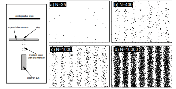
理论力学是研究物质的运动和导致这种运动的力量。它被应用于分析任何动态系统,从原子到太阳系。薄壁管的应力、变形和稳定性分析是物理学和工程学的一个经典课题。
statistics-lab™ 为您的留学生涯保驾护航 在代写理论力学Theoretical Mechanics方面已经树立了自己的口碑, 保证靠谱, 高质且原创的统计Statistics代写服务。我们的专家在代写理论力学Theoretical Mechanics代写方面经验极为丰富,各种代写理论力学Theoretical Mechanics相关的作业也就用不着说。
我们提供的理论力学Theoretical Mechanics及其相关学科的代写,服务范围广, 其中包括但不限于:
- Statistical Inference 统计推断
- Statistical Computing 统计计算
- Advanced Probability Theory 高等概率论
- Advanced Mathematical Statistics 高等数理统计学
- (Generalized) Linear Models 广义线性模型
- Statistical Machine Learning 统计机器学习
- Longitudinal Data Analysis 纵向数据分析
- Foundations of Data Science 数据科学基础
物理代写|理论力学作业代写Theoretical Mechanics代考|Trigonometric Functions
It can be assumed that the trigonometric functions are well-known from schoolmathematics. Therefore, only the most important relations shall be compiled in this subsection.
- Radian measure
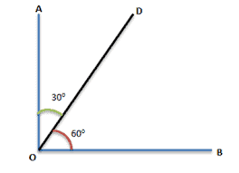
Figure $1.3$ illustrates that the angle $\varphi$ can be expressed not only by angular degrees $^{\circ}$, but equally uniquely also via the arc of the circle $s$ :
$$
s=s(\varphi) \quad: \quad s\left(360^{\circ}\right)=2 \pi r ; s\left(180^{\circ}\right)=\pi r ; s\left(90^{\circ}\right)=\frac{\pi}{2} r ; \ldots
$$
One introduces the dimensionless quantity
$$
\begin{gathered}
\varphi=\frac{s}{r} \quad \text { ‘radian’ } \
\varphi\left(^{\circ}\right)=360(180,90,45,1) \longrightarrow 2 \pi\left(\pi, \frac{\pi}{2}, \frac{\pi}{4}, \frac{\pi}{180}\right) \mathrm{rad}
\end{gathered}
$$ - Trigonometric functions
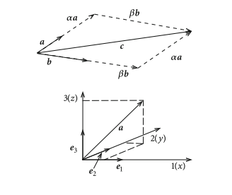
In the right-angled triangle in Fig. $1.4 a$ and $b$, adjacent and opposite to angle $\alpha$, respectively, are called the leg (side, cathetus) and $c$ the hypothenuse. With these terms one defines:
$$
\begin{aligned}
\sin \alpha &=\frac{b}{c} \
\cos \alpha &=\frac{a}{c} \
\tan \alpha &=\frac{\sin \alpha}{\cos \alpha}=\frac{b}{a} \
\cot \alpha &=\frac{\cos \alpha}{\sin \alpha}=\frac{1}{\tan \alpha}=\frac{a}{b}
\end{aligned}
$$
物理代写|理论力学作业代写Theoretical Mechanics代考|Exponential Function and Logarithm
- Exponential function
By this one understands the following function:
$$
y=a^{x} .
$$
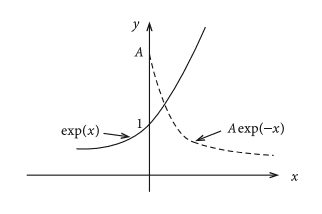
$a$ is called the ‘basis’ and $x$ the ‘exponent’. Here $a$ may be an arbitrary real number. Very often one uses Euler’s number e (1.18) writing:
$$
y=y_{0} e^{\alpha x}=y_{0} \exp (\alpha x)
$$
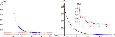
This function is of great importance in theoretical physics and appears often in a variety of contexts (rate of growth, increase of population, law of radioactive decay, capacitor charge and discharge, …) (Fig. 1.8).
In Sect. $1.1 .10$ we will be able to prove, by using the Taylor expansion, the following important series expansion of the exponential function:
$$
e^{x}=\sum_{n=0}^{\infty} \frac{x^{n}}{n !} .
$$
- Logarithm
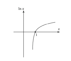
It is just the inverse function of $y=a^{x}$ being defined only for $y>0$ :
Logarithm to the base $a$
$$
x=\log {a} y . $$ Thus, if $a$ is raised to the power of $\log {a} y$ one gets $y$. Rather often one uses $a=10$ and calls it then ‘common (decimal) logarithm’:
$$
\log {10} 100=2 ; \log {10} 1000=3 ; \ldots
$$
However, in physics we use most frequently the ‘natural logarithm’ with base $a=e$ denoted by the symbol $\log _{e} \equiv \ln$. In this case the explicit indication of the base is left out:
$$
\ln \left(e^{x}\right)=x \Longleftrightarrow e^{\ln x}=x .
$$
理论力学代写
物理代写|理论力学作业代写Theoretical Mechanics代考|Trigonometric Functions
可以假设三角函数在学校数学中是众所周知的。因此,本小节只编写最重要的关系。
- 弧度测量
图 $1.3$ 说明角度 $\varphi$ 不仅可以用角度来表示,但同样独特地也通过圆弧 $s$ :
$$
s=s(\varphi) \quad: \quad s\left(360^{\circ}\right)=2 \pi r ; s\left(180^{\circ}\right)=\pi r ; s\left(90^{\circ}\right)=\frac{\pi}{2} r ; \ldots
$$
一、介绍无量纲量
$$
\varphi=\frac{s}{r} \quad \text { ‘radian’ } \varphi\left({ }^{\circ}\right)=360(180,90,45,1) \longrightarrow 2 \pi\left(\pi, \frac{\pi}{2}, \frac{\pi}{4}, \frac{\pi}{180}\right) \mathrm{rad}
$$ - 三角函数
在图 1 中的直角三角形中。 $1.4 a$ 和 $b$, 与角相邻且相反 $\alpha$, 分别称为腿 (side, cathetus) 和 $c$ 假设。使用这些术语 可以定义:
$$
\sin \alpha=\frac{b}{c} \cos \alpha \quad=\frac{a}{c} \tan \alpha=\frac{\sin \alpha}{\cos \alpha}=\frac{b}{a} \cot \alpha \quad=\frac{\cos \alpha}{\sin \alpha}=\frac{1}{\tan \alpha}=\frac{a}{b}
$$
物理代写|理论力学作业代写Theoretical Mechanics代考|Exponential Function and Logarithm
- 指数函数 由此理解以下函数:
$$
y=a^{x} .
$$
$a$ 被称为“基础”并且 $x$ “指数”。这里 $a$ 可以是任意实数。经常有人使用欧拉数 e (1.18) 写作:
$$
y=y_{0} e^{\alpha x}=y_{0} \exp (\alpha x)
$$
该函数在理论物理学中非常重要,并且经常出现在各种环境中 (增长率、人口增加、放射性衰变定律、电容器 充电和放电……) (图 1.8)。
昆虫。1.1.10我们将能够通过使用泰勒展开来证明指数函数的以下重要级数展开:
$$
e^{x}=\sum_{n=0}^{\infty} \frac{x^{n}}{n !} .
$$ - 对数
它只是的反函数 $y=a^{x}$ 仅被定义为 $y>0$ :
以对数为底 $a$
$$
x=\log a y .
$$
因此,如果 $a$ 被提升到 $\log a y$ 一个得到 $y$. 往往一种用途 $a=10$ 然后将其称为”常用 (十进制) 对数”:
$$
\log 10100=2 ; \log 101000=3 ; \ldots
$$
然而,在物理学中,我们最常使用带底的“自然对数” $a=e$ 用符号表示 $\log _{e} \equiv \ln$. 在这种情况下,基地的明确 指示被省略:
$$
\ln \left(e^{x}\right)=x \Longleftrightarrow e^{\ln x}=x .
$$

统计代写请认准statistics-lab™. statistics-lab™为您的留学生涯保驾护航。
金融工程代写
金融工程是使用数学技术来解决金融问题。金融工程使用计算机科学、统计学、经济学和应用数学领域的工具和知识来解决当前的金融问题,以及设计新的和创新的金融产品。
非参数统计代写
非参数统计指的是一种统计方法,其中不假设数据来自于由少数参数决定的规定模型;这种模型的例子包括正态分布模型和线性回归模型。
广义线性模型代考
广义线性模型(GLM)归属统计学领域,是一种应用灵活的线性回归模型。该模型允许因变量的偏差分布有除了正态分布之外的其它分布。
术语 广义线性模型(GLM)通常是指给定连续和/或分类预测因素的连续响应变量的常规线性回归模型。它包括多元线性回归,以及方差分析和方差分析(仅含固定效应)。
有限元方法代写
有限元方法(FEM)是一种流行的方法,用于数值解决工程和数学建模中出现的微分方程。典型的问题领域包括结构分析、传热、流体流动、质量运输和电磁势等传统领域。
有限元是一种通用的数值方法,用于解决两个或三个空间变量的偏微分方程(即一些边界值问题)。为了解决一个问题,有限元将一个大系统细分为更小、更简单的部分,称为有限元。这是通过在空间维度上的特定空间离散化来实现的,它是通过构建对象的网格来实现的:用于求解的数值域,它有有限数量的点。边界值问题的有限元方法表述最终导致一个代数方程组。该方法在域上对未知函数进行逼近。[1] 然后将模拟这些有限元的简单方程组合成一个更大的方程系统,以模拟整个问题。然后,有限元通过变化微积分使相关的误差函数最小化来逼近一个解决方案。
tatistics-lab作为专业的留学生服务机构,多年来已为美国、英国、加拿大、澳洲等留学热门地的学生提供专业的学术服务,包括但不限于Essay代写,Assignment代写,Dissertation代写,Report代写,小组作业代写,Proposal代写,Paper代写,Presentation代写,计算机作业代写,论文修改和润色,网课代做,exam代考等等。写作范围涵盖高中,本科,研究生等海外留学全阶段,辐射金融,经济学,会计学,审计学,管理学等全球99%专业科目。写作团队既有专业英语母语作者,也有海外名校硕博留学生,每位写作老师都拥有过硬的语言能力,专业的学科背景和学术写作经验。我们承诺100%原创,100%专业,100%准时,100%满意。
随机分析代写
随机微积分是数学的一个分支,对随机过程进行操作。它允许为随机过程的积分定义一个关于随机过程的一致的积分理论。这个领域是由日本数学家伊藤清在第二次世界大战期间创建并开始的。
时间序列分析代写
随机过程,是依赖于参数的一组随机变量的全体,参数通常是时间。 随机变量是随机现象的数量表现,其时间序列是一组按照时间发生先后顺序进行排列的数据点序列。通常一组时间序列的时间间隔为一恒定值(如1秒,5分钟,12小时,7天,1年),因此时间序列可以作为离散时间数据进行分析处理。研究时间序列数据的意义在于现实中,往往需要研究某个事物其随时间发展变化的规律。这就需要通过研究该事物过去发展的历史记录,以得到其自身发展的规律。
回归分析代写
多元回归分析渐进(Multiple Regression Analysis Asymptotics)属于计量经济学领域,主要是一种数学上的统计分析方法,可以分析复杂情况下各影响因素的数学关系,在自然科学、社会和经济学等多个领域内应用广泛。
MATLAB代写
MATLAB 是一种用于技术计算的高性能语言。它将计算、可视化和编程集成在一个易于使用的环境中,其中问题和解决方案以熟悉的数学符号表示。典型用途包括:数学和计算算法开发建模、仿真和原型制作数据分析、探索和可视化科学和工程图形应用程序开发,包括图形用户界面构建MATLAB 是一个交互式系统,其基本数据元素是一个不需要维度的数组。这使您可以解决许多技术计算问题,尤其是那些具有矩阵和向量公式的问题,而只需用 C 或 Fortran 等标量非交互式语言编写程序所需的时间的一小部分。MATLAB 名称代表矩阵实验室。MATLAB 最初的编写目的是提供对由 LINPACK 和 EISPACK 项目开发的矩阵软件的轻松访问,这两个项目共同代表了矩阵计算软件的最新技术。MATLAB 经过多年的发展,得到了许多用户的投入。在大学环境中,它是数学、工程和科学入门和高级课程的标准教学工具。在工业领域,MATLAB 是高效研究、开发和分析的首选工具。MATLAB 具有一系列称为工具箱的特定于应用程序的解决方案。对于大多数 MATLAB 用户来说非常重要,工具箱允许您学习和应用专业技术。工具箱是 MATLAB 函数(M 文件)的综合集合,可扩展 MATLAB 环境以解决特定类别的问题。可用工具箱的领域包括信号处理、控制系统、神经网络、模糊逻辑、小波、仿真等。