statistics-lab™ 为您的留学生涯保驾护航 在代写代考有限元方法Finite Element Method方面已经树立了自己的口碑, 保证靠谱, 高质量且原创的统计Statistics和数学Math代写服务。我们的专家在代考有限元方法Finite Element Method代写方面经验极为丰富,各种代写有限元方法Finite Element Method相关的作业也就用不着说。
问题 1. a. Demonstrate the effects of the time step on the solution for a case where $\alpha=0, \beta=1 / 2, \gamma=1 / 4$,
Solution of part (a): In case the numerical integration parameters are chosen as $\alpha=0, \beta=1 / 2$, $\gamma=\frac{1}{4}$, the $\alpha$-method presents an unconditionally stable and implicit solution algorithm. The transient solutions presented in are
obtained by using $\Delta t=10^{-1}, 10^{-2}, 10^{-3}$, and $10^{-4}$ second-time steps. This figure compares the numerically calculated solution to the analytically predicted solution given in ; vibration response of the mid-point of the beam (top) and the vibration snapshots (bottom) of the whole beam are plotted as a function of time. We see that the solution remains stable for all four time step sizes, but the coarsest time step, $\Delta t=10^{-1}$, has significant period and amplitude errors. By using smaller time steps, the error is diminished significantly. For the case of $\Delta t=10^{-4}$, the numerical and analytical solutions become virtually identical.
最后的总结:
通过对有限元方法Finite Element Method各方面的介绍,想必您对这门课有了初步的认识。如果你仍然不确定或对这方面感到困难,你仍然可以依靠我们的代写和辅导服务。我们拥有各个领域、具有丰富经验的专家。他们将保证你的 essay、assignment或者作业都完全符合要求、100%原创、无抄袭、并一定能获得高分。需要如何学术帮助的话,随时联系我们的客服。
Combinatorial problems have been studied since ancient times, but combinatorics as an important field of mathematics has only been recognized in the last fifty years. The first article focusing on combinatorics was by Netto. Combinatorics gained a certain autonomy after Percy Alexander MacMahon published Combinatorial Analysis in 1915. Over the following years its importance gradually grew: König’s texts on graph theory and Marshall Hall should be remembered.
Its development was stimulated by the work of Gian-Carlo Rota, who from the 1960s contributed to the basis of a wide-ranging and clearly formalized unified theory. Another influential figure was Marcel Paul Schuzenberg. A different but very effective action was attributed to Paul Erdős and his ability to raise and solve problems, his contribution mainly concerned extreme problems.
For $n$ and $r$ positive integers with $r \leq n$, $$ P(n, r)=n \times(n-1) \times \cdots \times(n-r+1) . $$
Proof. In constructing an $r$-permutation of an $n$-element set, we can choose the first item in $n$ ways, the second item in $n-1$ ways, whatever the choice of the first item, . . . , and the $r$ th item in $n-(r-1)$ ways, whatever the choice of the first $r-1$ items. By the multiplication principle the $r$ items can be chosen in $n \times(n-1) \times \cdots \times(n-r+1)$ ways. For a nonnegative integer $n$, we define $n !($ read $n$ factorial $)$ by $$ n !=n \times(n-1) \times \cdots \times 2 \times 1, $$ with the convention that $0 !=1$. We may then write $$ P(n, r)=\frac{n !}{(n-r) !} . $$ For $n \geq 0$, we define $P(n, 0)$ to be 1 , and this agrees with the formula when $r=0$. The number of permutations of $n$ elements is $$ P(n, n)=\frac{n !}{0 !}=n ! $$
In Europe, Bonaventure Cavalieri laid the foundations of differential and integral calculus by discussing in his dissertation the method of determining the area and volume as the sum of the areas and volumes of very fine regions.
His work on the formulation of the calculus led to the combination of Cavalieri’s calculus with the finite difference method, which appeared in Europe at about the same time. This integration was carried out by John Wallis, Isaac Barrow, and James Gregory, with Barrow and Gregory proving the Second Theorem of the Fundamental Theorem of Calculus around 1675.
Isaac Newton introduced the concepts of the law of product differentiation, the chain rule, higher-order differential notation, Taylor series, and analytic functions in a unique notation, and used them to solve problems in mathematical physics. At the time of publication, Newton replaced differentiation with equivalent geometric subjects to accommodate the mathematical terminology of the time and to avoid censure. In Mathematical Principles of Natural Philosophy, Newton used differential and integral methods to discuss a variety of problems, including the orbits of celestial bodies, the shapes of the surfaces of rotating fluids, the eccentricity of the earth, and the motion of a heavy object sliding on a pendulum. In addition to this, Newton developed the series expansion of functions, and it is clear that he understood the principles of Taylor’s series.
Gottfried Leibniz was initially suspected of plagiarizing Newton’s unpublished papers, but is now recognized as one of the original contributors to the development of calculus. It was Gottfried Leibniz who systematized these ideas and established calculus as a rigorous discipline. At the time, he was accused of plagiarizing Newton, but today he is recognized as one of the original contributors to the establishment and development of differential and integral calculus. Leibniz explicitly defined the rules for the operation of differentials, made possible the computation of second- and higher-order derivatives, and defined Leibniz’s law and the chain rule. Unlike Newton, Leibniz was very much a formalist and spent many days agonizing over what symbols to use for each concept.
Let $P=(0,1,0), Q=(2,1,3), R=(1,-1,2)$. Compute $\overrightarrow{P Q} \times \overrightarrow{P R}$ and find the equation of the plane through $P, Q$, and $R$, in the form $a x+b y+c z=d$.
$\overrightarrow{P Q}=\langle 2,0,3\rangle ; \overrightarrow{P R}=\langle 1,-2,2\rangle ; \overrightarrow{P Q} \times \overrightarrow{P R}=\left|\begin{array}{ccc}\hat{\imath} & \hat{\jmath} & k \ 2 & 0 & 3 \ 1 & -2 & 2\end{array}\right|=6 \hat{\imath}-\hat{\jmath}-4 \hat{\boldsymbol{k}}$ Equation of the plane: $6 x-y-4 z=d$. Plane passing through $P: 6 \cdot 0-1-4 \cdot 0=d$. Equation of the plane: $6 x-y-4 z=-1$.
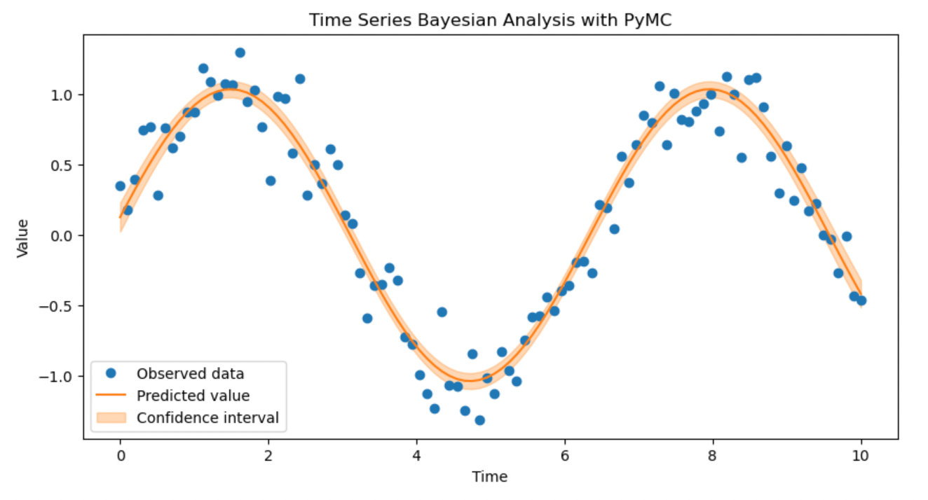
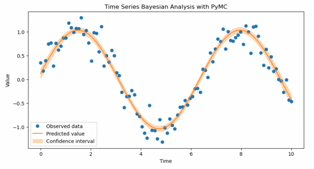
statistics-lab™ 为您的留学生涯保驾护航 在代写代考时间序列分析Time Series Analysis方面已经树立了自己的口碑, 保证靠谱, 高质量且原创的统计Statistics和数学Math代写服务。我们的专家在代考时间序列分析Time Series Analysis代写方面经验极为丰富,各种代写时间序列分析Time Series Analysis相关的作业也就用不着说。
For an $A R(1)$ process the optimal forecast $k$ periods in the future is: $$ E_t\left[Y_{t+k}\right]=\phi^k Y_t $$
Proof. For an $\mathrm{AR}(1)$ process we have shifting (2.6) $k$ periods in the future that: $$ Y_{t+k}=\phi Y_{t+k-1}+a_{t+k} . $$ Applying $E_t$ to both sides we obtain: $$ E_t\left[Y_{t+k}\right]=\phi E_t\left[Y_{t+k-1}\right]+\underbrace{E_t\left[a_{t+k}\right]}{=0} $$ where: $E_t\left[a{t+k}\right]=0$ since $a_{t+k}$ is $i . i . d$. and hence independent of the information at time $t$. Hence: $$ E_t\left[Y_{t+k}\right]=\phi \underbrace{E_t\left[Y_{t+k-1}\right]}{=\phi E_t\left[Y{t+k-2}\right]} . $$ Continuing this process of substitution we have: $$ E_t\left[Y_{t+k}\right]=\phi^k E_t\left[Y_t\right] . $$ Since $Y_t$ is observed at time $t$ and is thus in the information set, it follows that: $$ E_t\left[Y_t\right]=Y_t $$
最后的总结:
通过对时间序列分析Time Series Analysis各方面的介绍,想必您对这门课有了初步的认识。如果你仍然不确定或对这方面感到困难,你仍然可以依靠我们的代写和辅导服务。我们拥有各个领域、具有丰富经验的专家。他们将保证你的 essay、assignment或者作业都完全符合要求、100%原创、无抄袭、并一定能获得高分。需要如何学术帮助的话,随时联系我们的客服。
Consider the following Bayesian model: $$ \begin{aligned} & (y \mid \theta) \sim \operatorname{Binomial}(n, \theta) \ & \theta \sim \operatorname{Beta}(\alpha, \beta) \quad \text { (prior). } \end{aligned} $$ Find the posterior distribution of $\theta$.
The posterior density is $$ \begin{aligned} f(\theta \mid y) \propto f(\theta) f(y \mid \theta) & \ & =\frac{\theta^{\alpha-1}(1-\theta)^{\beta-1}}{B(\alpha, \beta)} \times\left(\begin{array}{l} n \ y \end{array}\right) \theta^y(1-\theta)^{n-y} \ & \propto \theta^{\alpha-1}(1-\theta)^{\beta-1} \times \theta^y(1-\theta)^{n-y} \quad \text { ignoring constants which } \ & =\theta^{(\alpha+y)-1}(1-\theta)^{(\beta+n-y)-1}, 0<\theta<1 . \end{aligned} $$ This is the kernel of the beta density with parameters $\alpha+y$ and $\beta+n-y$. It follows that the posterior distribution of $\theta$ is given by $$ (\theta \mid y) \sim \operatorname{Beta}(\alpha+y, \beta+n-y), $$ and the posterior density of $\theta$ is (exactly) $$ f(\theta \mid y)=\frac{\theta^{(\alpha+y)-1}(1-\theta)^{(\beta+n-y)-1}}{B(\alpha+y, \beta+n-y)}, 0<\theta<1 . $$ For example, suppose that $\alpha=\beta=1$, that is, $\theta \sim \operatorname{Beta}(1,1)$. Then the prior density is $f(\theta)=\frac{\theta^{1-1}(1-\theta)^{1-1}}{B(1,1)}=1,0<\theta<1$. Thus the prior may also be expressed by writing $\theta \sim U(0,1)$. Also, suppose that $n=2$. Then there are three possible values of $y$, namely 0,1 and 2 , and these lead to the following three posteriors, respectively: $$ \begin{aligned} & (\theta \mid y) \sim \operatorname{Beta}(1+0,1+2-0)=\operatorname{Beta}(1,3) \ & (\theta \mid y) \sim \operatorname{Beta}(1+1,1+2-1)=\operatorname{Beta}(2,2) \ & (\theta \mid y) \sim \operatorname{Beta}(1+2,1+2-2)=\operatorname{Beta}(3,1) . \end{aligned} $$
安托万-奥古斯丁-库尔诺(Antoine Augustin Cournot)1838 年发表在他的《财富理论的数学原理研究》(Recherches sur les principes mathématiques de la théorie des richesses)一书中对双人博弈的分析,可以看作是纳什均衡概念在特定背景下的首次表述。
约翰-冯-诺依曼 1944 年,约翰-冯-诺依曼(John von Neumann)和奥斯卡-摩根斯特恩(Oskar Morgenstern)出版了《博弈与经济行为理论》(Theory of Games and Economic Behavior)一书,博弈论由此成为一个独立的研究领域。这部开创性著作详细介绍了解决零和博弈的方法。
Every finite strategic-form game has a mixedstrategy equilibrium.
Remark Remember that a pure-strategy equilibrium is an equilibrium in degenerate mixed strategies. The theorem does not assert the existence of an equilibrium with nondegenerate mixing.
Proof Since this is the archetypal existence proof in game theory, we will go through it in detail. The idea of the proof is to apply Kakutani’s fixed-point theorem to the players’ “reaction correspondences.” Player $i$ ‘s reaction correspondence, $r_i$, maps each strategy profilc $\sigma$ to the set of mixed strategies that maximize player $i$ ‘s payoff when his opponents play $\sigma_i$. (Although $r_i$ depends only on $\sigma_{-i}$ and not on $\sigma_i$, we write it as a function of the strategies of all players. because later we will look for a fixed point in the space $\Sigma$ of strategy profiles.) This is the natural generalization of the Cournot reaction function we defined above. Define the correspondence $r: \Sigma \rightrightarrows \Sigma$ to be the Cartesian product of the $r_i$. A fixed point of $r$ is a $\sigma$ such that $\sigma \in r(\sigma)$, so that, for each player, $\sigma_i \in r_i(\sigma)$. Thus, a fixed point of $r$ is a Nash equilibrium.
From Kakutani’s theorem, the following are sufficient conditions for $r: \Sigma \rightrightarrows \Sigma$ to have a fixed point: (1) $\Sigma$ is a compact, ${ }^{17}$ convex,${ }^{18}$ nonempty subset of a (finite-dimensional) Fuclidean space. (2) $r(\sigma)$ is nonempty for all $\sigma$. (3) $r(\sigma)$ is convex for all $\sigma$.
(4) $r(\cdot)$ has a closed graph: If $\left(\sigma^n, \hat{\sigma}^n\right) \rightarrow(\sigma, \hat{\sigma})$ with $\hat{\sigma}^n \in r\left(\sigma^n\right)$, then $\hat{\sigma} \in r(\sigma)$. (This property is also often referred to as upper hemi-continuity. ${ }^{19}$ ) Let us check that these conditions are satisfied. Condition 1 is easy – each $\Sigma_i$ is a simplex of dimension $\left(# S_i-1\right)$. Each player’s payoff function is linear, and therefore continuous in his own mixed strategy, and since continuous functions on compact sets attain maxima, condition 2 is satisfied. If $r(\sigma)$ were not convex, there would be a $\sigma^{\prime} \in r(\sigma)$, a $\sigma^{\prime \prime} \in r(\sigma)$, and a $\lambda \in(0,1)$ such that $\lambda \sigma^{\prime}+(1-\lambda) \sigma^{\prime \prime} \notin r(\sigma)$. But for each player $i$, $$ u_i\left(j \sigma_i^{\prime}+(1-i) \sigma_i^{\prime \prime}, \sigma_{-i}\right)=\lambda u_i\left(\sigma_i^{\prime}, \sigma_{-i}\right)+(1-\lambda) u_i\left(\sigma_i^{\prime \prime}, \sigma_{-i}\right), $$ so that if both $\sigma_i^{\prime}$ and $\sigma_i^{\prime \prime}$ are best responses to $\sigma_{-i}$, then so is their weighted average. This verifics condition 3 .
Finally, assume that condition 4 is violated so there is a sequence $\left(\sigma^n, \hat{\sigma}^n\right) \rightarrow(\sigma, \hat{\sigma}), \hat{\sigma}^n \in r\left(\sigma^n\right)$, but $\hat{\sigma} \notin r(\sigma)$. Then $\hat{\sigma}i \notin r_i(\sigma)$ for some player $i$. Thus, there is an $z>0$ and a $\sigma_i^{\prime}$ such that $u_i\left(\sigma_i^{\prime}, \sigma{-i}\right)>u_i\left(\hat{\sigma}i, \sigma{-i}\right)+3 \varepsilon$. Since $u_i$ is continuous and $\left(\sigma^n, \hat{\sigma}^n\right) \rightarrow(\sigma, \hat{\sigma})$, for $n$ sufficiently large we have $$ u_i\left(\sigma_i^{\prime}, \sigma_{-i}^n\right)>u_i\left(\sigma_i^{\prime}, \sigma_{-i}\right)-\varepsilon>u_i\left(\hat{\sigma}i, \sigma{-i}\right)+2 \varepsilon>u_i\left(\hat{\sigma}i^n, \sigma{-i}^n\right)+\varepsilon . $$
statistics-labTM为您提供多伦多大学 (University of Toronto)Statistical Inference 统计推理加拿大代写代考和辅导服务!
课程介绍:
The course surveys the various approaches that have been considered for the development of a theory of statistical reasoning. These include likelihood methods, Bayesian methods and frequentism. These are compared with respect to their strengths and weaknesses. To use statistics successfully requires a clear understanding of the meaning of various concepts such as likelihood, confidence, p-value, belief, etc. This is the purpose of the course.
STAC58H|Statistical Inference 统计推理 多伦多大学
Statistical Inference 统计推论案例
问题 1.
Accounting for voter turnout. Let $N$ be the number of people in the state of Iowa. Suppose $p N$ of these people support Hillary Clinton, and $(1-p) N$ of them support Donald Trump, for some $p \in(0,1) . N$ is known (say $N=3,000,000)$ and $p$ is unknown. (a) Suppose that each person in Iowa randomly and independently decides, on election day, whether or not to vote, with probability $1 / 2$ of voting and probability $1 / 2$ of not voting. Let $V_{\text {Hillary }}$ be the number of people who vote for Hillary and $V_{\text {Donald }}$ be the number of people who vote for Donald. Show that $$ \mathbb{E}\left[V_{\text {Hillary }}\right]=\frac{1}{2} p N, \quad \mathbb{E}\left[V_{\text {Donald }}\right]=\frac{1}{2}(1-p) N . $$ What are the standard deviations of $V_{\text {Hillary }}$ and $V_{\text {Donald }}$, in terms of $p$ and $N$ ? Explain why, when $N$ is large, we expect the fraction of voters who vote for Hillary to be very close to $p$.
(a) Recall that a $\operatorname{Binomial}(n, p)$ random variable has mean $n p$ and variance $n p(1-p)$. A total of $p N$ people support Hillary, each voting independently with probability $\frac{1}{2}$, so $V_{\text {Hillary }} \sim \operatorname{Binomial}\left(p N, \frac{1}{2}\right)$. Then $$ \mathbb{E}\left[V_{\text {Hillary }}\right]=\frac{1}{2} p N, \quad \operatorname{Var}\left[V_{\text {Hillary }}\right]=\frac{1}{4} p N, $$ and the standard deviation of $V_{\text {Hillary }}$ is $\sqrt{\frac{1}{4} p N}$. Similarly, as $(1-p) N$ people support Donald, $V_{\text {Donald }} \sim \operatorname{Binomial}\left((1-p) N, \frac{1}{2}\right)$, so $$ \mathbb{E}\left[V_{\text {Donald }}\right]=\frac{1}{2}(1-p) N, \quad \operatorname{Var}\left[V_{\text {Donald }}\right]=\frac{1}{4}(1-p) N, $$ and the standard deviation of $V_{\text {Donald }}$ is $\sqrt{\frac{1}{4}(1-p) N}$. The fraction of voters who vote for Hillary is $$ \frac{V_{\text {Hillary }}}{V_{\text {Hillary }}+V_{\text {Donald }}}=\frac{V_{\text {Hillary }} / N}{V_{\text {Hillary }} / N+V_{\text {Donald }} / N} . $$ As $\mathbb{E}\left[V_{\text {Hillary }} / N\right]=\frac{1}{2} p$ (a constant) and $\operatorname{Var}\left[V_{\text {Hillary }} / N\right]=\frac{1}{4} p / N \rightarrow 0$ as $N \rightarrow \infty$, $V_{\text {Hillary }} / N$ should be close to $\frac{1}{2} p$ with high probability when $N$ is large. Similarly, as $\mathbb{E}\left[V_{\text {Donald }} / N\right]=\frac{1}{2}(1-p)$ and $\operatorname{Var}\left[V_{\text {Donald }} / N\right]=\frac{1}{4}(1-p) / N \rightarrow 0$ as $N \rightarrow \infty$, $V_{\text {Donald }} / N$ should be close to $\frac{1}{2}(1-p)$ with high probability when $N$ is large. Then the fraction of voters for Hillary should, with high probability, be close to $$ \frac{\frac{1}{2} p}{\frac{1}{2} p+\frac{1}{2}(1-p)}=p . $$ (The above statements “close to with high probability” may be formalized using Chebyshev’s inequality, which states that a random variable is, with high probability, not too many standard deviations away from its mean.)
问题 2.
(b) Now suppose there are two types of voters – “passive” and “active”. Each passive voter votes on election day with probability $1 / 4$ and doesn’t vote with probability $3 / 4$, while each active voter votes with probability $3 / 4$ and doesn’t vote with probability $1 / 4$. Suppose that a fraction $q_H$ of the people who support Hillary are passive and $1-q_H$ are active, and a fraction $q_D$ of the people who support Donald are passive and $1-q_D$ are active. Show that $$ \mathbb{E}\left[V_{\text {Hillary }}\right]=\frac{1}{4} q_H p N+\frac{3}{4}\left(1-q_H\right) p N, \quad \mathbb{E}\left[V_{\text {Donald }}\right]=\frac{1}{4} q_D(1-p) N+\frac{3}{4}\left(1-q_D\right)(1-p) N . $$ What are the standard deviations of $V_{\text {Hillary }}$ and $V_{\text {Donald }}$, in terms of $p, N, q_H$, and $q_D$ ? If we estimate $p$ by $\hat{p}$ using a simple random sample of $n=1000$ people from Iowa, as discussed in Lecture 1, explain why $\hat{p}$ might not be a good estimate of the fraction of voters who will vote for Hillary.
(b) Let $V_{\mathrm{H}, \mathrm{p}}$ and $V_{\mathrm{H}, \mathrm{a}}$ be the number of passive and active voters who vote for Hillary, and similarly define $V_{\mathrm{D}, \mathrm{p}}$ and $V_{\mathrm{D}, \mathrm{a}}$ for Donald. There are $q_H p N$ passive Hillary supporters, each of whom vote independently with probability $\frac{1}{4}$, so $$ V_{\mathrm{H}, \mathrm{p}} \sim \operatorname{Binomial}\left(q_H p N, \frac{1}{4}\right) . $$
Similarly, $$ \begin{aligned} V_{\mathrm{H}, \mathrm{a}} & \sim \operatorname{Binomial}\left(\left(1-q_H\right) p N, \frac{3}{4}\right), \ V_{\mathrm{D}, \mathrm{P}} & \sim \operatorname{Binomial}\left(q_D(1-p) N, \frac{1}{4}\right), \ V_{\mathrm{D}, \mathrm{a}} & \sim \operatorname{Binomial}\left(\left(1-q_D\right)(1-p) N, \frac{3}{4}\right), \end{aligned} $$ and these four random variables are independent. Since $V_{\mathrm{Hillary}}=V_{\mathrm{H}, \mathrm{p}}+V_{\mathrm{H}, \mathrm{a}}$, $$ \begin{aligned} \mathbb{E}\left[V_{\text {Hillary }}\right] & =\mathbb{E}\left[V_{\mathrm{H}, \mathrm{p}}\right]+\mathbb{E}\left[V_{\mathrm{H}, \mathrm{a}}\right]=\frac{1}{4} q_H p N+\frac{3}{4}\left(1-q_H\right) p N, \ \operatorname{Var}\left[V_{\text {Hillary }}\right] & =\operatorname{Var}\left[V_{\mathrm{H}, \mathrm{p}}\right]+\operatorname{Var}\left[V_{\mathrm{H}, \mathrm{a}}\right]=\frac{3}{16} q_H p N+\frac{3}{16}\left(1-q_H\right) p N=\frac{3}{16} p N, \end{aligned} $$ and the standard deviation of $V_{\text {Hillary }}$ is $\sqrt{\frac{3}{16} p N}$. Similarly, $$ \begin{aligned} \mathbb{E}\left[V_{\text {Donald }}\right] & =\mathbb{E}\left[V_{\mathrm{D}, \mathrm{p}}\right]+\mathbb{E}\left[V_{\mathrm{D}, \mathrm{a}}\right]=\frac{1}{4} q_D(1-p) N+\frac{3}{4}\left(1-q_D\right)(1-p) N, \ \operatorname{Var}\left[V_{\text {Donald }}\right] & =\operatorname{Var}\left[V_{\mathrm{D}, \mathrm{p}}\right]+\operatorname{Var}\left[V_{\mathrm{D}, \mathrm{a}}\right]=\frac{3}{16} q_D(1-p) N+\frac{3}{16}\left(1-q_D\right)(1-p) N \ & =\frac{3}{16}(1-p) N, \end{aligned} $$ and the standard deviation of $V_{\text {Donald }}$ is $\sqrt{\frac{3}{16}(1-p) N}$. The quantity $\hat{p}$ estimates $p$, but in this case $p$ may not be the fraction of voters who vote for Hillary: By the same argument as in part (a), the fraction of voters who vote for Hillary is given by $$ \begin{aligned} \frac{V_{\text {Hillary }}}{V_{\text {Hillary }}+V_{\text {Donald }}} & =\frac{V_{\text {Hillary }} / N}{V_{\text {Hillary }} / N+V_{\text {Donald }} / N} \ & \approx \frac{\frac{1}{4} q_H p+\frac{3}{4}\left(1-q_H\right) p}{\frac{1}{4} q_H p+\frac{3}{4}\left(1-q_H\right) p+\frac{1}{4} q_D(1-p)+\frac{3}{4}\left(1-q_D\right)(1-p)}, \end{aligned} $$ where the approximation is accurate with high probability when $N$ is large. When $q_H \neq q_D$, this is different from $p$ : For example, if $q_H=0$ and $q_D=1$, this is equal to $\frac{p}{p+(1-p) / 3}$ which is greater than $p$, reflecting the fact that Hillary supporters are more likely to vote than are Donald supporters.
问题 3.
(c) We do not know $q_H$ and $q_D$. However, suppose that in our simple random sample, we can observe whether each person is passive or active, in addition to asking them whether they support Hillary or Donald. ${ }^1$ Suggest estimators $\hat{V}{\text {Hillary }}$ and $\hat{V}{\text {Donald }}$ for $\mathbb{E}\left[V_{\text {Hillary }}\right]$ and $\mathbb{E}\left[V_{\text {Donald }}\right]$ using this additional information. Show, for your estimators, that $$ \mathbb{E}\left[\hat{V}{\text {Hillary }}\right]=\frac{1}{4} q_H p N+\frac{3}{4}\left(1-q_H\right) p N, \quad \mathbb{E}\left[\hat{V}{\text {Donald }}\right]=\frac{1}{4} q_D(1-p) N+\frac{3}{4}\left(1-q_D\right)(1-p) N $$
(c) Let $\hat{p}$ be the proportion of the 1000 surveyed people who support Hillary. Among the surveyed people supporting Hillary, let $\hat{q}H$ be the proportion who are passive. Similarly, among the surveyed people supporting Donald, let $\hat{q}_D$ be the proportion who are passive. (Note that these are observed quantities, computed from our sample of 1000 people.) Then we may estimate the number of voters for Hillary and Donald by $$ \begin{aligned} \hat{V}{\text {Hillary }} & =\frac{1}{4} \hat{q}H \hat{p} N+\frac{3}{4}\left(1-\hat{q}_H\right) \hat{p} N \ \hat{V}{\text {Donald }} & =\frac{1}{4} \hat{q}_D(1-\hat{p}) N+\frac{3}{4}\left(1-\hat{q}_D\right)(1-\hat{p}) N . \end{aligned} $$
$\hat{q}H \hat{p}$ is simply the proportion of the 1000 surveyed people who both support Hillary and are passive. Hence, letting $X_1, \ldots, X{1000}$ indicate whether each surveyed person both supports Hillary and is passive, we have $$ \hat{q}H \hat{p}=\frac{1}{n}\left(X_1+\ldots+X_n\right) . $$ Each $X_i \sim \operatorname{Bernoulli}\left(q_H p\right)$, so linearity of expectation implies $\mathbb{E}\left[\hat{q}_H \hat{p}\right]=q_H p$. Similarly, $\left(1-\hat{q}_H\right) \hat{p}, \hat{q}_D(1-\hat{p})$, and $\left(1-\hat{q}_D\right)(1-\hat{p})$ are the proportions of the 1000 surveyed people who support Hillary and are active, support Donald and are passive, and support Donald and are active, so the same argument shows $\mathbb{E}\left[\left(1-\hat{q}_H\right) \hat{p}\right]=\left(1-q_H\right) p, \mathbb{E}\left[\hat{q}_D(1-\hat{p})\right]=q_D(1-p)$, and $\mathbb{E}\left[\left(1-\hat{q}_D\right)(1-\hat{p})\right]=$ $\left(1-q_D\right)(1-p)$. Then applying linearity of expectation again yields $$ \mathbb{E}\left[\hat{V}{\text {Hillary }}\right]=\mathbb{E}\left[V_{\text {Hillary }}\right], \quad \mathbb{E}\left[\hat{V}{\text {Donald }}\right]=\mathbb{E}\left[V{\text {Donald }}\right] . $$
In today’s data-rich world more and more people from diverse fields are needing to perform statistical analyses and indeed more and more tools for doing so are becoming available; it is relatively easy to point and click and obtain some statistical analysis of your data. But how do you know if any particular analysis is indeed appropriate? Is there another procedure or workflow which would be more suitable? Is there such thing as a best possible approach in a given situation? All of these questions (and more) are addressed in this unit. You will study the foundational core of modern statistical inference, including classical and cutting-edge theory and methods of mathematical statistics with a particular focus on various notions of optimality. The first part of the unit covers various aspects of distribution theory which are necessary for the second part which deals with optimal procedures in estimation and testing. The framework of statistical decision theory is used to unify many of the concepts. You will rigorously prove key results and apply these to real-world problems in laboratory sessions. By completing this unit you will develop the necessary skills to confidently choose the best statistical analysis to use in many situations.
Suppose that grades on a midterm and final have a correlation coefficient of 0.6 and both exams have an average score of 75 . and a standard deviation of 10 . (a). If a student’s score on the midterm is 90 what would you predict her score on the final to be?
Solution: (a). Let $x$ be the midterm score and $y$ be the final score. The least-squares regression of $y$ on $x$ is given in terms of the standardized values: $$ \frac{\hat{y}-\bar{y}}{s_y}=r \frac{x-\bar{x}}{s_x} $$ A score of 90 on the midterm is $(90-75) / 10=1.5$ standard deviations above the mean. The predicted score on the final will be $r \times 1.5=.9$ standard deviations above the mean final score, which is $75+(.9) \times 10=84$.
问题 2.
(b). If a student’s score on the final was 75 , what would you guess that his score was on the midterm?
(b). For this case we need to regress the midterm score $(x)$ on (y). The same argument in (a), reversing $x$ and $y$ leads to: $$ \frac{\hat{x}-\bar{x}}{s_x}=r \frac{y-\bar{y}}{s_y} $$ Since the final score was 75 , which is zero-standard deviations above $\bar{y}$, the prediction of the midterm score is $\bar{x}=75$.
问题 3.
(c). Consider all students scoring at the 75 th percentile or higher on the midterm. What proportion of these students would you expect to be at or above the 75 th percentile of the final? (i) $75 \%$, (ii) $50 \%$, (iii) less than $50 \%$, or (iv) more than $50 \%$.
(c). By the regression effect we expect dependent variable scores to be closer to their mean in standard-deviation units than the independdent variable is to its mean, in standard-deviation units. Since the 75 th percentile is on the midterm is above the mean, we expect these students to have average final score which is lower than the 75 th percentile (i.e., closer to the mean). This means (iii) is the correct answer.
statistics-lab™ 为您的留学生涯保驾护航 在代写有限元法 Finite Element Method(FEM)方面已经树立了自己的口碑, 保证靠谱, 高质量且原创的统计Statistics和数学Math代写服务。我们的专家在代写有限元法 Finite Element Method(FEM)代写方面经验极为丰富,各种代写有限元法 Finite Element Method(FEM)相关的作业也就用不着说。
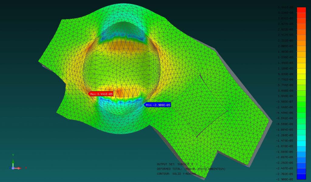
Equation of motion of a solid bar a) Derive the equation of motion of an elastic bar in terms of its deflection $u(x, t)$. Initially, assume that the bar has a variable cross-sectional area $A(x)$ and that it is subjected to distributed axial load $q(x, t)$ and a concentrated force $F$ at its free end as shown in Fig. 1.2. Also assume small deflections, linear elastic material behavior with constant elastic modulus $E$, and constant mass density $\rho$.
The solution domain $\Omega$ for this problem spans $0<x<L$. The boundaries $\Gamma$ of the solution domain are located at $x=0$ and $x=L$. Internal forces develop in the bar in response to external loading. The internal normal force $N(x)$ at the cross-section $x$ can be defined as follows: $$ N(x)=\bar{\sigma}(x) A(x) $$ where the average normal stress $\bar{\sigma}$ is defined as follows: $$ \bar{\sigma}(x)=\frac{1}{A(x)} \int_{A(x)} \sigma d A $$ and where $\sigma$ is the internal normal stress, $A$ is the cross-sectional area of the bar. The equation of motion of the bar can be obtained by using Newton’s second law on a small segment of the bar (Fig. 1.2). The balance of internal and inertial forces gives, $$ \begin{aligned} & \sum F_x=\rho A d x \frac{\partial^2 u}{\partial t^2} \ & -N+q d x+\left(N+\frac{\partial N}{\partial x} d x\right)=\rho A d x \frac{\partial^2 u}{\partial t^2} \ & \frac{\partial N}{\partial x}=-q+\rho A \frac{\partial^2 u}{\partial t^2} \end{aligned} $$ (b) Hooke’s law defines the constitutive relationship between the internal stress and strain for linear, elastic materials. For a slender bar, the Hooke’s law can be given as follows: $$ \bar{\sigma}=E \varepsilon $$ where $E$ is the elastic (Young’s) modulus of the material. The straindisplacement, $\varepsilon-u$, relationship is given as follows: $$ \varepsilon=\frac{\partial u}{\partial x} $$
Hooke’s law defines the constitutive relationship between the internal stress and strain for linear, elastic materials. For a slender bar, the Hooke’s law can be given as follows: $$ \bar{\sigma}=E \varepsilon $$ where $E$ is the elastic (Young’s) modulus of the material. The straindisplacement, $\varepsilon-u$, relationship is given as follows: $$ \varepsilon=\frac{\partial u}{\partial x} $$ Combining Eqs. (1.6-1.9), we find the internal force resultant as follows: $$ N=\bar{\sigma} A=E A \frac{\partial u}{\partial x} $$ The equation of motion can then be found by combining Eqs. (1.7c) and (1.10), $$ \frac{\partial}{\partial x}\left[E A \frac{\partial u}{\partial x}\right]=-q+\rho A \frac{\partial^2 u}{\partial t^2} $$
This is a PDE that governs the dynamics of axial deflection $u(x, t)$ along the bar. Its solution requires two boundary conditions and two initial conditions. The boundaries of this bar are located at $x=0, L$. At the $x=L$ boundary, the force resultant should be equal to the applied load, i.e., $N(L)=F$. By using Eq. (1.10), this condition can be expressed in terms of the bar deflection. The boundary
conditions for this problem then become, Boundary conditions: $u(0)=0$ (a) $$ \left.\frac{\partial u}{\partial x}\right|{x=L}=\frac{F}{E A(L)} $$ The initial conditions represent the state of deflection and velocity of the entire bar at $t=0$. In general, these conditions can be represented as follows: $$ \text { Initial conditions: } \begin{aligned} u(x, 0) & =u^{(0)}(x) \ \left.\frac{\partial u}{\partial t}\right|{t=0} & =\dot{u}^{(0)}(x) \end{aligned} $$ where $u^{(0)}(x)$ and $\dot{u}^{(0)}(x)$ are known functions.
最后的总结:
通过对有限元法Finite Element Method(FEM)各方面的介绍,想必您对组合学有了初步的认识。有限元法Finite Element Method(FEM)对于学习数学知识起到了至关重要的作用。所以一定要打好坚实的基础去准备学习这门课程。但如果你仍然不确定或对这方面感到困难,你仍然可以依靠我们的代写和辅导服务。我们拥有各个领域、具有丰富经验的专家。他们将保证你的 essay、assignment或者作业都完全符合要求、100%原创、无抄袭、并一定能获得高分。需要如何学术帮助的话,随时联系我们的客服。