如果你也在 怎样代写离散数学discrete mathematics这个学科遇到相关的难题，请随时右上角联系我们的24/7代写客服。

离散数学是研究可以被认为是 “离散”（类似于离散变量，与自然数集有偏射）而不是 “连续”（类似于连续函数）的数学结构。离散数学研究的对象包括整数、图形和逻辑中的语句。相比之下，离散数学不包括 “连续数学 “中的课题，如实数、微积分或欧几里得几何。离散对象通常可以用整数来列举；更正式地说，离散数学被定性为处理可数集的数学分支（有限集或与自然数具有相同心数的集）。然而，”离散数学 “这一术语并没有确切的定义。

statistics-lab™ 为您的留学生涯保驾护航 在代写离散数学discrete mathematics方面已经树立了自己的口碑, 保证靠谱, 高质且原创的统计Statistics代写服务。我们的专家在代写离散数学discrete mathematics代写方面经验极为丰富，各种代写离散数学discrete mathematics相关的作业也就用不着说。

我们提供的离散数学discrete mathematics及其相关学科的代写，服务范围广, 其中包括但不限于:

• Statistical Inference 统计推断
• Statistical Computing 统计计算
• Advanced Probability Theory 高等概率论
• Advanced Mathematical Statistics 高等数理统计学
• (Generalized) Linear Models 广义线性模型
• Statistical Machine Learning 统计机器学习
• Longitudinal Data Analysis 纵向数据分析
• Foundations of Data Science 数据科学基础

数学代写|离散数学作业代写discrete mathematics代考|Greatest Common Divisors and Least Common Multiples

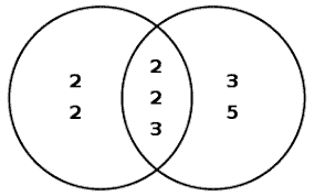
The greatest common divisor (gcd) of two nonzero integers $a$ and $b$, denoted by $\operatorname{gcd}(a, b)$, is the largest integer $d$ such that $d \mid a$ and $d \mid b$, except that $\operatorname{gcd}(0,0)=0$. Note that if $\operatorname{gcd}(a, b)=d$, then $\operatorname{gcd}\left(\frac{a}{d}, \frac{b}{d}\right)=1$. For instance, the set of divisors of 24 is ${1,2,3,4,6,8,12,24}$ and the set of divisors of 42 is ${1,2,3,6,7,14,21}$. Because the set of common divisors is ${1,2,3,6}$, we have $\operatorname{gcd}(24,42)=6$, also $\operatorname{gcd}\left(\frac{24}{6}, \frac{42}{6}\right)=\operatorname{gcd}(4,7)=1$

The integers $a$ and $b$ are relatively prime if their gad is 1 . For instance, neither 15 nor 16 is prime; however, 15 and 16 are relatively prime, as their gcd is 1 . In addition, integers are called pairwise relatively prime if the gcd of any two integers is 1 . For instance, none of the integers 25,26 , and 27 is prime, yet they are pairwise relatively prime.

The gcd of two nonzero integers exists if the set of their common divisors is nonempty and finite. The methods to determine the gcd of two integers $a$ and $b$ are as follows:

Brute-force method: First, find all the positive divisors of each integer, then determine the set of all common divisors of both integers, and finally select the largest common divisor in the set.

数学代写|离散数学作业代写discrete mathematics代考|Divisibility Test

A divisibility test is a quick way to determine whether an integer, called dividend, is divisible by a smaller integer, called divisor, without performing the division. The test is usually based on the examination of the digits of the dividend in a way that solely depends on what the divisor is. Consider an integer $a$ with $n$ digits $\left{a_{n-1}, a_{n-2}, \ldots, a_1, a_0\right}$ whose decimal representation is then as follows:
$$
a=a_{n-1}\left(10^{n-1}\right)+a_{n-2}\left(10^{n-2}\right)+\ldots+a_1\left(10^1\right)+a_0\left(10^0\right) .
$$
Note that $a_0$ is the least significant digit and $a_{n-1}$ is the most significant digit. As an example, we have $71524=7 \times\left(10^4\right)+1 \times\left(10^3\right)+5 \times\left(10^2\right)+2 \times\left(10^1\right)+$ $4 \times\left(10^{\circ}\right)$, where the least significant digit is 4 and the most significant digit is 7 .
The divisibility rules for dividing an integer $a$ by the integers $1,2,3,4,5,6,7,8,9$, or 10 are as follows:

Divisibility by 1: $1 \mid a \rightarrow$ No special condition on the coefficients $a_{n-1}, a_{n-2}, \ldots, a_0$ (i.e., every integer is divisible by 1 ).
Divisibility by 2: $2 \mid a \rightarrow a \bmod 2=a_0 \bmod 2=0 \rightarrow a_0 \in{0,2,4,6,8}$ (i.e., the least significant digit must be even).
Divisibility by 3: $3 \mid a \rightarrow a \bmod 3=\left(a_{n-1}+a_{n-2}, \ldots+a_0\right) \bmod 3=0$ (i.e., the sum of all digits must be divisible by 3 ).
Divisibility by 4: $4 \mid a \rightarrow a \bmod 4=\left(a_1\left(10^1\right)+a_0\left(10^0\right)\right) \bmod 4=0$ (i.e., the number representing the last two digits must be divisible by 4).
Divisibility by 5: $5 \mid a \rightarrow a \bmod 5=a_0 \bmod 5=0$ (i.e., the last digit must be a 0 or a 5 ).
Divisibility by 6: 6|a $\rightarrow a \bmod 6=0 \rightarrow a \bmod 2=0$ and $a \bmod 3=0$ (i.e., the integer must be divisible by both 2 and 3$)$.
Divisibility by $\quad 7: \quad 7 \mid a \rightarrow a \bmod 7=\left(\left(a_{n-1}\left(10^{n-2}\right)+a_{n-2}\left(10^{n-3}\right)+\ldots+\right.\right.$ $\left.\left.a_1\left(10^0\right)\right)-2\left(a_0\right)\right) \bmod 7=0$. Note that the process may need to be repeated.
Divisibility by 8: $8 \mid a \rightarrow a \bmod 8=\left(a_2\left(10^2\right)+a_1\left(10^1\right)+a_0\left(10^0\right)\right) \bmod 8=0$ (i.e., the number representing the last three digits must be divisible by 8 ).
Divisibility by 9: $9 \mid a \rightarrow a \bmod 9=\left(a_{n-1}+a_{n-2}, \ldots+a_0\right) \bmod 9=0$ (i.e., the sum of all digits must be divisible by 9$)$.
Divisibility by 10: $10 \mid a \rightarrow a \bmod 10=a_0 \bmod 10=0$ (i.e., the last digit must be a 0 ).
Note that for some divisors, such as 7 , there are multiple rules of divisibility, and only one of them is given here. Moreover, applying the divisibility by 7 to a large dividend may require several iterations (i.e., the process needs to be repeated until the divisibility becomes obvious). In addition, there are divisibility rules for notable prime divisors greater than 10 , such as 11,13 , and beyond.

离散数学代写

数学代写|离散数学作业代写discrete mathematics代考|Greatest Common Divisors and Least Common Multiples

两个非零整数的最大公约数 (gcd) $a$ 和 $b$ ，表示为 $\operatorname{gcd}(a, b)$, 是最大的整数 $d$ 这样 $d \mid a$ 和 $d \mid b$ ， 除了那个 $\operatorname{gcd}(0,0)=0$. 请注意，如果 $\operatorname{gcd}(a, b)=d$ ，然后 $\operatorname{gcd}\left(\frac{a}{d}, \frac{b}{d}\right)=1$. 例如， 24 的 除数集合是 $1,2,3,4,6,8,12,2442$ 的除数集合是 $1,2,3,6,7,14,21$. 因为公约数的集合是 $1,2,3,6$ ，我们有 $\operatorname{gcd}(24,42)=6$ ，还 $\operatorname{gcd}\left(\frac{24}{6}, \frac{42}{6}\right)=\operatorname{gcd}(4,7)=1$
整数 $a$ 和 $b$ 如果它们的 gad 是 1 ，则它们是互质的。例如， 15 和 16 都不是素数；然而， 15 和 16 互质，因为它们的 $\operatorname{gcd}$ 是 1 。此外，如果任意两个整数的 $\operatorname{gcd}$ 为 1 ，则整数被称为成对相 对质数。例如，整数 25,26 和 27 都不是质数，但它们成对互质。
如果两个非零整数的公约数的集合是非空且有限的，则它们的 $\operatorname{gcd}$ 存在。确定两个整数的gcd 的方法 $a$ 和 $b$ 如下面所述:
蛮力法: 首先找出每个整数的所有正约数，然后确定两个整数的所有公约数的集合，最后在集 合中选出最大公约数。

数学代写|离散数学作业代写discrete mathematics代考|Divisibility Test

可除性测试是一种快速确定整数 (称为被除数) 是否可被较小整数（称为除数）整除的快速方 法，无需执行除法。该测试通常基于对被除数数字的检查，其方式完全取决于除数是多少。考 虑一个整数 $a$ 和 $n$ 数字 Veft{a_{n-1}, a_{n-2}, Vdots, a_1, a_0iright} 其十进制表示如下:
$$
a=a_{n-1}\left(10^{n-1}\right)+a_{n-2}\left(10^{n-2}\right)+\ldots+a_1\left(10^1\right)+a_0\left(10^0\right) .
$$
注意 $a_0$ 是最低有效数字并且 $a_{n-1}$ 是最重要的数字。例如，我们有 $71524=7 \times\left(10^4\right)+1 \times\left(10^3\right)+5 \times\left(10^2\right)+2 \times\left(10^1\right)+4 \times\left(10^{\circ}\right)$ ，其中最低 有效数字为 4 ，最高有效数字为 7 。
整除整数的整除法则 $a$ 由整数 $1,2,3,4,5,6,7,8,9$ ，或 10 个如下:
被 1 整除: $1 \mid a \rightarrow$ 系数无特殊条件 $a_{n-1}, a_{n-2}, \ldots, a_0$ （即，每个整数都可以被 1 整 除) 。
被 2 整除: $2 \mid a \rightarrow a \bmod 2=a_0 \bmod 2=0 \rightarrow a_0 \in 0,2,4,6,8$ (即，最低有效位 必须是偶数）。
被 3 整除: $3 \mid a \rightarrow a \bmod 3=\left(a_{n-1}+a_{n-2}, \ldots+a_0\right) \bmod 3=0$ (即，所有数字的 总和必须能被 3 整除) 。
被 4 整除: $4 \mid a \rightarrow a \bmod 4=\left(a_1\left(10^1\right)+a_0\left(10^0\right)\right) \bmod 4=0$ (即表示最后两位 数的数字必须能被 4 整除) 。
被 5 整除: $5 \mid a \rightarrow a \bmod 5=a_0 \bmod 5=0$ （即，最后一位数字必须是 0 或 5 ）。
被6整除: $6 \mid \mathrm{a} \rightarrow a \bmod 6=0 \rightarrow a \bmod 2=0$ 和 $a \bmod 3=0$ (即整数必须能被 2 和 3 整除).
整除性 $7: \quad 7 \mid a \rightarrow a \bmod 7=\left(\left(a_{n-1}\left(10^{n-2}\right)+a_{n-2}\left(10^{n-3}\right)+\ldots+\right.\right.$ $\left.\left.a_1\left(10^0\right)\right)-2\left(a_0\right)\right) \bmod 7=0$. 请注意，该过程可能需要重复。
被 8 整除: $8 \mid a \rightarrow a \bmod 8=\left(a_2\left(10^2\right)+a_1\left(10^1\right)+a_0\left(10^0\right)\right) \bmod 8=0$
(即 代表最后三位数字的数字必须能被 8 整除)。
被 9 整除: $9 \mid a \rightarrow a \bmod 9=\left(a_{n-1}+a_{n-2}, \ldots+a_0\right) \bmod 9=0$ (即所有数字的和 必须能被 9 整除).
被 10 整除: $10 \mid a \rightarrow a \bmod 10=a_0 \bmod 10=0$ (即，最后一位数字必须是 0 ）。 请注意，对于一些除数，例如 7 ，有多种整除规则，这里只给出其中一种。此外，将被 7 整除 的能力应用到大股息可能需要多次迭代 (即，需要重复该过程，直到整除性变得明显)。此 外，对于大于 10 的显着素因数（例如 11,13 及以上），还有整除规则。

统计代写请认准statistics-lab™. statistics-lab™为您的留学生涯保驾护航。

金融工程代写

金融工程是使用数学技术来解决金融问题。金融工程使用计算机科学、统计学、经济学和应用数学领域的工具和知识来解决当前的金融问题，以及设计新的和创新的金融产品。

非参数统计代写

非参数统计指的是一种统计方法，其中不假设数据来自于由少数参数决定的规定模型；这种模型的例子包括正态分布模型和线性回归模型。

广义线性模型代考

广义线性模型（GLM）归属统计学领域，是一种应用灵活的线性回归模型。该模型允许因变量的偏差分布有除了正态分布之外的其它分布。

术语 广义线性模型（GLM）通常是指给定连续和/或分类预测因素的连续响应变量的常规线性回归模型。它包括多元线性回归，以及方差分析和方差分析（仅含固定效应）。

有限元方法代写

有限元方法（FEM）是一种流行的方法，用于数值解决工程和数学建模中出现的微分方程。典型的问题领域包括结构分析、传热、流体流动、质量运输和电磁势等传统领域。

有限元是一种通用的数值方法，用于解决两个或三个空间变量的偏微分方程（即一些边界值问题）。为了解决一个问题，有限元将一个大系统细分为更小、更简单的部分，称为有限元。这是通过在空间维度上的特定空间离散化来实现的，它是通过构建对象的网格来实现的：用于求解的数值域，它有有限数量的点。边界值问题的有限元方法表述最终导致一个代数方程组。该方法在域上对未知函数进行逼近。[1] 然后将模拟这些有限元的简单方程组合成一个更大的方程系统，以模拟整个问题。然后，有限元通过变化微积分使相关的误差函数最小化来逼近一个解决方案。

tatistics-lab作为专业的留学生服务机构，多年来已为美国、英国、加拿大、澳洲等留学热门地的学生提供专业的学术服务，包括但不限于Essay代写，Assignment代写，Dissertation代写，Report代写，小组作业代写，Proposal代写，Paper代写，Presentation代写，计算机作业代写，论文修改和润色，网课代做，exam代考等等。写作范围涵盖高中，本科，研究生等海外留学全阶段，辐射金融，经济学，会计学，审计学，管理学等全球99%专业科目。写作团队既有专业英语母语作者，也有海外名校硕博留学生，每位写作老师都拥有过硬的语言能力，专业的学科背景和学术写作经验。我们承诺100%原创，100%专业，100%准时，100%满意。

随机分析代写

随机微积分是数学的一个分支，对随机过程进行操作。它允许为随机过程的积分定义一个关于随机过程的一致的积分理论。这个领域是由日本数学家伊藤清在第二次世界大战期间创建并开始的。

时间序列分析代写

随机过程，是依赖于参数的一组随机变量的全体，参数通常是时间。 随机变量是随机现象的数量表现，其时间序列是一组按照时间发生先后顺序进行排列的数据点序列。通常一组时间序列的时间间隔为一恒定值（如1秒，5分钟，12小时，7天，1年），因此时间序列可以作为离散时间数据进行分析处理。研究时间序列数据的意义在于现实中，往往需要研究某个事物其随时间发展变化的规律。这就需要通过研究该事物过去发展的历史记录，以得到其自身发展的规律。

回归分析代写

多元回归分析渐进（Multiple Regression Analysis Asymptotics）属于计量经济学领域，主要是一种数学上的统计分析方法，可以分析复杂情况下各影响因素的数学关系，在自然科学、社会和经济学等多个领域内应用广泛。

MATLAB代写

MATLAB 是一种用于技术计算的高性能语言。它将计算、可视化和编程集成在一个易于使用的环境中，其中问题和解决方案以熟悉的数学符号表示。典型用途包括：数学和计算算法开发建模、仿真和原型制作数据分析、探索和可视化科学和工程图形应用程序开发，包括图形用户界面构建MATLAB 是一个交互式系统，其基本数据元素是一个不需要维度的数组。这使您可以解决许多技术计算问题，尤其是那些具有矩阵和向量公式的问题，而只需用 C 或 Fortran 等标量非交互式语言编写程序所需的时间的一小部分。MATLAB 名称代表矩阵实验室。MATLAB 最初的编写目的是提供对由 LINPACK 和 EISPACK 项目开发的矩阵软件的轻松访问，这两个项目共同代表了矩阵计算软件的最新技术。MATLAB 经过多年的发展，得到了许多用户的投入。在大学环境中，它是数学、工程和科学入门和高级课程的标准教学工具。在工业领域，MATLAB 是高效研究、开发和分析的首选工具。MATLAB 具有一系列称为工具箱的特定于应用程序的解决方案。对于大多数 MATLAB 用户来说非常重要，工具箱允许您学习和应用专业技术。工具箱是 MATLAB 函数（M 文件）的综合集合，可扩展 MATLAB 环境以解决特定类别的问题。可用工具箱的领域包括信号处理、控制系统、神经网络、模糊逻辑、小波、仿真等。

R语言代写	问卷设计与分析代写
PYTHON代写	回归分析与线性模型代写
MATLAB代写	方差分析与试验设计代写
STATA代写	机器学习/统计学习代写
SPSS代写	计量经济学代写
EVIEWS代写	时间序列分析代写
EXCEL代写	深度学习代写
SQL代写	各种数据建模与可视化代写

如果你也在 怎样代写离散数学discrete mathematics这个学科遇到相关的难题，请随时右上角联系我们的24/7代写客服。

离散数学是研究可以被认为是 “离散”（类似于离散变量，与自然数集有偏射）而不是 “连续”（类似于连续函数）的数学结构。离散数学研究的对象包括整数、图形和逻辑中的语句。相比之下，离散数学不包括 “连续数学 “中的课题，如实数、微积分或欧几里得几何。离散对象通常可以用整数来列举；更正式地说，离散数学被定性为处理可数集的数学分支（有限集或与自然数具有相同心数的集）。然而，”离散数学 “这一术语并没有确切的定义。

statistics-lab™ 为您的留学生涯保驾护航 在代写离散数学discrete mathematics方面已经树立了自己的口碑, 保证靠谱, 高质且原创的统计Statistics代写服务。我们的专家在代写离散数学discrete mathematics代写方面经验极为丰富，各种代写离散数学discrete mathematics相关的作业也就用不着说。

我们提供的离散数学discrete mathematics及其相关学科的代写，服务范围广, 其中包括但不限于:

• Statistical Inference 统计推断
• Statistical Computing 统计计算
• Advanced Probability Theory 高等概率论
• Advanced Mathematical Statistics 高等数理统计学
• (Generalized) Linear Models 广义线性模型
• Statistical Machine Learning 统计机器学习
• Longitudinal Data Analysis 纵向数据分析
• Foundations of Data Science 数据科学基础

数学代写|离散数学作业代写discrete mathematics代考|Matrix Inversion

A square matrix $\boldsymbol{A}$ is said to be invertible if there exists a square matrix $\boldsymbol{B}$ such that
$$
A B=B A=I \rightarrow B=A^{-1} \& A=B^{-1}
$$
where the matrix $\boldsymbol{B}$ is called the inverse of the matrix $\boldsymbol{A}$ and denoted by $\boldsymbol{A}^{-1}$. If $\boldsymbol{B}$ is the inverse of $\boldsymbol{A}$, then $\boldsymbol{A}$ is the inverse of $\boldsymbol{B}$. A square matrix that is not invertible is called singular. Note that if a matrix is not square, then it has no inverse. In addition, a product of invertible matrices is always invertible, and the inverse of the product is the product of the inverses in the reverse order, that is, we have $(A B)^{-1}=B^{-1} A^{-1}$. The inverse of the matrix $A$ plays much the same role in matrix algebra that the reciprocal of a number plays in the arithmetic of real numbers.

An effective method to find the inverse of a matrix is to employ the elementary row operations. The elementary row operations consist of the following suboperations:

• Interchange two rows.
• Multiply all entries in a row by a nonzero number.
• Add a multiple of a row to another row.
  To find the inverse of the matrix $A$ of size $n$ using the elementary row operations, we take the following steps:

1. Form the $n \times 2 n$ matrix $(\boldsymbol{A}, \boldsymbol{I})$, that is, the matrix $A$ is in the left half of it and the identity matrix $\boldsymbol{I}$ is in its right half.

数学代写|离散数学作业代写discrete mathematics代考|Zero-One Matrix

Assuming $a$ and $b$ are binary digits, also known as bits $(0$ or 1$)$, the Boolean operations $V$ and $\wedge$ are defined as follows:
$$
a \vee b= \begin{cases}0 & \text { if } a=b=0 \ 1 & \text { otherwise }\end{cases}
$$
and
$$
a \wedge b= \begin{cases}1 & \text { if } a=b=1 \ 0 & \text { otherwise }\end{cases}
$$
A matrix whose entries are either 0 or 1 and subject to the Boolean operations is called a zero-one matrix, Boolean matrix, or logical matrix. Let $\boldsymbol{A}$ and $\boldsymbol{B}$ be zero-one matrices of the same size. The join of $\boldsymbol{A}$ and $\boldsymbol{B}$, denoted by $\boldsymbol{A} \vee \boldsymbol{B}$, and the meet of $\boldsymbol{A}$ and $\boldsymbol{B}$, denoted by $\boldsymbol{A} \wedge \boldsymbol{B}$, are defined respectively as follows:
$$
\boldsymbol{A} \vee \boldsymbol{B}=\left(a_{i j} \vee b_{i j}\right)
$$
and
$$
\boldsymbol{A} \wedge \boldsymbol{B}=\left(a_{i j} \wedge b_{i j}\right)
$$
Let $\boldsymbol{A}=\left(a_{i j}\right)$ be an $m \times n$ zero-one matrix and $\boldsymbol{B}=\left(b_{i j}\right)$ be an $n \times r$ zero-one matrix. The Boolean product of $\boldsymbol{A}$ and $\boldsymbol{B}$, denoted by $\boldsymbol{A} \odot \boldsymbol{B}$, is the $m \times r$ zero-one matrix $C=\left(c_{i j}\right)$, where we have the following:
$$
\boldsymbol{A} \odot \boldsymbol{B}=\boldsymbol{C} \rightarrow\left(c_{i k}\right)=\left(\left(a_{i 1} \wedge b_{1 k}\right) \vee \ldots \vee\left(a_{i n} \wedge b_{n k}\right)\right), \quad i=1, \ldots, m \& k=1, \ldots, r .
$$
The Boolean product is obtained in the same fashion as the ordinary product of matrices where addition and multiplication are replaced with the operations $\vee$ and $\wedge$ respectively, noting that the Boolean product can be obtained by finding the usual product of matrices and then replacing any nonzero integer by 1 .

离散数学代写

数学代写|离散数学作业代写discrete mathematics代考|Matrix Inversion

方阵 $\boldsymbol{A}$ 如果存在方阵，则称它是可逆的 $\boldsymbol{B}$ 这样
$$
A B=B A=I \rightarrow B=A^{-1} \& A=B^{-1}
$$
其中矩阵 $\boldsymbol{B}$ 称为矩阵的逆 $\boldsymbol{A}$ 并表示为 $\boldsymbol{A}^{-1}$. 如果 $\boldsymbol{B}$ 是的倒数 $\boldsymbol{A}$ ，然后 $\boldsymbol{A}$ 是的倒数 $\boldsymbol{B}$. 不可逆的方阵称为 奇异矩阵。请注意，如果矩阵不是方阵，则它没有逆矩阵。此外，可逆矩阵的乘积总是可逆的，乘积的 逆是倒序逆序的乘积，即我们有 $(A B)^{-1}=B^{-1} A^{-1}$. 矩阵的逆 $A$ 在矩阵代数中扮演的角色与数的倒数 在实数算术中扮演的角色非常相似。
求逆矩阵的一种有效方法是使用基本行运算。基本行操作由以下子操作组成:

• 交换两行。
• 将一行中的所有条目乘以一个非零数。
• 将一行的倍数添加到另一行。 找到矩阵的逆 $A$ 尺寸 $n$ 使用基本行操作，我们采取以下步骤:

1. 形成 $n \times 2 n$ 矩阵 $(\boldsymbol{A}, \boldsymbol{I})$, 即矩阵 $A$ 在它的左半部分和单位矩阵 $\boldsymbol{I}$ 在它的右半边。

数学代写|离散数学作业代写discrete mathematics代考|Zero-One Matrix

假设 $a$ 和 $b$ 是二进制数字，也称为位 $(0$ 或 1$)$ ，布尔运算 $V$ 和八定义如下:
$a \vee b={0 \quad$ if $a=b=01 \quad$ otherwise
和
$a \wedge b={1 \quad$ if $a=b=10 \quad$ otherwise
其元素为 0 或 1 并进行布尔运算的矩阵称为零一矩阵、布尔矩阵或逻辑矩阵。让 $\boldsymbol{A}$ 和 $\boldsymbol{B}$ 是大小相同的零 一矩阵。的加入 $\boldsymbol{A}$ 和 $\boldsymbol{B}$, 表示为 $\boldsymbol{A} \vee \boldsymbol{B}$ ，和满足 $\boldsymbol{A}$ 和 $\boldsymbol{B}$ ， 表示为 $\boldsymbol{A} \wedge \boldsymbol{B}$ ， 分别定义如下:
$$
\boldsymbol{A} \vee \boldsymbol{B}=\left(a_{i j} \vee b_{i j}\right)
$$
和
$$
\boldsymbol{A} \wedge \boldsymbol{B}=\left(a_{i j} \wedge b_{i j}\right)
$$
让 $\boldsymbol{A}=\left(a_{i j}\right)$ 豆 $m \times n$ 零一矩阵和 $\boldsymbol{B}=\left(b_{i j}\right)$ 豆 $n \times r$ 零一矩阵。的布尔积 $\boldsymbol{A}$ 和 $\boldsymbol{B}$, 表示为 $\boldsymbol{A} \odot \boldsymbol{B}$ ， 是个 $m \times r$ 零一矩阵 $C=\left(c_{i j}\right)$ ，我们有以下内容:
$$
\boldsymbol{A} \odot \boldsymbol{B}=\boldsymbol{C} \rightarrow\left(c_{i k}\right)=\left(\left(a_{i 1} \wedge b_{1 k}\right) \vee \ldots \vee\left(a_{i n} \wedge b_{n k}\right)\right), \quad i=1, \ldots, m \& k=1, \ldots, r
$$
布尔积的获得方式与矩阵的普通积相同，其中加法和乘法被运算替换 $V$ 和 $\wedge$ 分别指出布尔积可以通过找到 矩阵的通常积然后用 1 替换任何非零整数来获得。

统计代写请认准statistics-lab™. statistics-lab™为您的留学生涯保驾护航。

金融工程代写

金融工程是使用数学技术来解决金融问题。金融工程使用计算机科学、统计学、经济学和应用数学领域的工具和知识来解决当前的金融问题，以及设计新的和创新的金融产品。

非参数统计代写

非参数统计指的是一种统计方法，其中不假设数据来自于由少数参数决定的规定模型；这种模型的例子包括正态分布模型和线性回归模型。

广义线性模型代考

广义线性模型（GLM）归属统计学领域，是一种应用灵活的线性回归模型。该模型允许因变量的偏差分布有除了正态分布之外的其它分布。

术语 广义线性模型（GLM）通常是指给定连续和/或分类预测因素的连续响应变量的常规线性回归模型。它包括多元线性回归，以及方差分析和方差分析（仅含固定效应）。

有限元方法代写

有限元方法（FEM）是一种流行的方法，用于数值解决工程和数学建模中出现的微分方程。典型的问题领域包括结构分析、传热、流体流动、质量运输和电磁势等传统领域。

有限元是一种通用的数值方法，用于解决两个或三个空间变量的偏微分方程（即一些边界值问题）。为了解决一个问题，有限元将一个大系统细分为更小、更简单的部分，称为有限元。这是通过在空间维度上的特定空间离散化来实现的，它是通过构建对象的网格来实现的：用于求解的数值域，它有有限数量的点。边界值问题的有限元方法表述最终导致一个代数方程组。该方法在域上对未知函数进行逼近。[1] 然后将模拟这些有限元的简单方程组合成一个更大的方程系统，以模拟整个问题。然后，有限元通过变化微积分使相关的误差函数最小化来逼近一个解决方案。

tatistics-lab作为专业的留学生服务机构，多年来已为美国、英国、加拿大、澳洲等留学热门地的学生提供专业的学术服务，包括但不限于Essay代写，Assignment代写，Dissertation代写，Report代写，小组作业代写，Proposal代写，Paper代写，Presentation代写，计算机作业代写，论文修改和润色，网课代做，exam代考等等。写作范围涵盖高中，本科，研究生等海外留学全阶段，辐射金融，经济学，会计学，审计学，管理学等全球99%专业科目。写作团队既有专业英语母语作者，也有海外名校硕博留学生，每位写作老师都拥有过硬的语言能力，专业的学科背景和学术写作经验。我们承诺100%原创，100%专业，100%准时，100%满意。

随机分析代写

随机微积分是数学的一个分支，对随机过程进行操作。它允许为随机过程的积分定义一个关于随机过程的一致的积分理论。这个领域是由日本数学家伊藤清在第二次世界大战期间创建并开始的。

时间序列分析代写

随机过程，是依赖于参数的一组随机变量的全体，参数通常是时间。 随机变量是随机现象的数量表现，其时间序列是一组按照时间发生先后顺序进行排列的数据点序列。通常一组时间序列的时间间隔为一恒定值（如1秒，5分钟，12小时，7天，1年），因此时间序列可以作为离散时间数据进行分析处理。研究时间序列数据的意义在于现实中，往往需要研究某个事物其随时间发展变化的规律。这就需要通过研究该事物过去发展的历史记录，以得到其自身发展的规律。

回归分析代写

多元回归分析渐进（Multiple Regression Analysis Asymptotics）属于计量经济学领域，主要是一种数学上的统计分析方法，可以分析复杂情况下各影响因素的数学关系，在自然科学、社会和经济学等多个领域内应用广泛。

MATLAB代写

MATLAB 是一种用于技术计算的高性能语言。它将计算、可视化和编程集成在一个易于使用的环境中，其中问题和解决方案以熟悉的数学符号表示。典型用途包括：数学和计算算法开发建模、仿真和原型制作数据分析、探索和可视化科学和工程图形应用程序开发，包括图形用户界面构建MATLAB 是一个交互式系统，其基本数据元素是一个不需要维度的数组。这使您可以解决许多技术计算问题，尤其是那些具有矩阵和向量公式的问题，而只需用 C 或 Fortran 等标量非交互式语言编写程序所需的时间的一小部分。MATLAB 名称代表矩阵实验室。MATLAB 最初的编写目的是提供对由 LINPACK 和 EISPACK 项目开发的矩阵软件的轻松访问，这两个项目共同代表了矩阵计算软件的最新技术。MATLAB 经过多年的发展，得到了许多用户的投入。在大学环境中，它是数学、工程和科学入门和高级课程的标准教学工具。在工业领域，MATLAB 是高效研究、开发和分析的首选工具。MATLAB 具有一系列称为工具箱的特定于应用程序的解决方案。对于大多数 MATLAB 用户来说非常重要，工具箱允许您学习和应用专业技术。工具箱是 MATLAB 函数（M 文件）的综合集合，可扩展 MATLAB 环境以解决特定类别的问题。可用工具箱的领域包括信号处理、控制系统、神经网络、模糊逻辑、小波、仿真等。

R语言代写	问卷设计与分析代写
PYTHON代写	回归分析与线性模型代写
MATLAB代写	方差分析与试验设计代写
STATA代写	机器学习/统计学习代写
SPSS代写	计量经济学代写
EVIEWS代写	时间序列分析代写
EXCEL代写	深度学习代写
SQL代写	各种数据建模与可视化代写

如果你也在 怎样代写离散数学discrete mathematics这个学科遇到相关的难题，请随时右上角联系我们的24/7代写客服。

离散数学是研究可以被认为是 “离散”（类似于离散变量，与自然数集有偏射）而不是 “连续”（类似于连续函数）的数学结构。离散数学研究的对象包括整数、图形和逻辑中的语句。相比之下，离散数学不包括 “连续数学 “中的课题，如实数、微积分或欧几里得几何。离散对象通常可以用整数来列举；更正式地说，离散数学被定性为处理可数集的数学分支（有限集或与自然数具有相同心数的集）。然而，”离散数学 “这一术语并没有确切的定义。

statistics-lab™ 为您的留学生涯保驾护航 在代写离散数学discrete mathematics方面已经树立了自己的口碑, 保证靠谱, 高质且原创的统计Statistics代写服务。我们的专家在代写离散数学discrete mathematics代写方面经验极为丰富，各种代写离散数学discrete mathematics相关的作业也就用不着说。

我们提供的离散数学discrete mathematics及其相关学科的代写，服务范围广, 其中包括但不限于:

• Statistical Inference 统计推断
• Statistical Computing 统计计算
• Advanced Probability Theory 高等概率论
• Advanced Mathematical Statistics 高等数理统计学
• (Generalized) Linear Models 广义线性模型
• Statistical Machine Learning 统计机器学习
• Longitudinal Data Analysis 纵向数据分析
• Foundations of Data Science 数据科学基础

数学代写|离散数学作业代写discrete mathematics代考|Propositional Equivalences

It is sometimes important to replace a logical statement with an equivalent statement in a mathematical argument. One method to determine whether two compound propositions are equivalent is to use well-known logical identities to establish new logical identities. This method is quite effective, especially when there are a large number of propositional variables involved. Table $1.12$ presents some important logical equivalences involving the negation, conjunction, and disjunction operators. Of all logical equivalences, De Morgan’s laws are of great importance, as they have wide applications in logic. De Morgan’s laws state that (1) the negation of an “and” statement is logically equivalent to the “or” statement in which each component is negated, and (2) the negation of an “or” statement is logically equivalent to the “and” statement in which each component is negated.

Table $1.13$ presents some important logical equivalences involving conditional and biconditional statements.

A compound proposition that is always true, regardless of the truth values of the propositional variables (i.e., the compound proposition contains only $\mathrm{T}$ in the last column of its truth table), is called a tautology. In other words, a tautology is an always-true proposition regardless of the truth values of the propositional variables. A statement whose form is a tautology is a tautological statement. Note that the compound propositions $p$ and $q$ are logically equivalent if $p \leftrightarrow q$ is a tautology. Some simple examples of tautology in English are “Parents are older than their children,” “You don’t give what you don’t have,” and “Dead people do not breathe.” A simple example of tautology in logic is $p \vee \bar{p}$.

A compound proposition that is always false, regardless of the truth values of the propositional variables (i.e., the compound proposition contains only $\mathrm{F}$ in the last column of its truth table), is called a contradiction. In other words, a contradiction is an alwaysfalse proposition regardless of the truth values of the propositional variables. A statement whose form is a contradiction is a contradictory statement. Note that the negation of a tautology is a contradiction, and the negation of a contradiction is a tautology. Some simple examples of contradiction in English are “Some are more equal than others,” “Rich people need a tax cut because they do not have enough money,” and “Texting while driving reduces chances of having a car accident.” A simple example of contradiction in logic is $p \wedge \bar{p}$.

Note that a compound proposition that is neither a tautology nor a contradiction is called a contingency. In most practical applications and statements in logic, the proposition happens to be contingency. A statement whose form is a contingency is a contingent statement. Some simplé examples of contingèncy in English aré “Politicians aré dishonest” and “People in this country are not racist.” A simple example of contingency in logic is $p \rightarrow \bar{p}$.

数学代写|离散数学作业代写discrete mathematics代考|Predicates

To understand predicate logic, we first need to understand the concept of a predicate. A predicate refers to the part of a sentence that attributes a property to the subject. For instance, in the sentence “The United States of America is a powerful country,” “The United States of America” is the subject, and the part of the sentence from which the subject has been removed (i.e., “is a powerful country”) is the predicate. Another example is the sentence ” $x$ represents the world population”, in which the variable ” $x$ ” is the subject and “represents the world population” is the predicate.

A predicate contains a finite number of variables and becomes a propositional statement when specific values are substituted for the variables. The domain, also known as the universe of discourse or the domain of discourse, is the set of all values of a variable that can replace it.

A predicate that involves just one variable may be denoted by $P(x)$. The statement $P(x)$ is said to be the value of the propositional function $P$ at $x$. A propositional function $P$, by itself, is neither true nor false. However, once a value from the domain has been assigned to the variable $x, P(x)$ becomes a propositional statement and thus has a truth value.

As stated earlier, by assigning a value to the variable $x$, the propositional function $P(x)$ becomes a propositional statement with a truth value. Another way to obtain a proposition from a propositional function is to add quantifiers. For instance, the propositions “Few people are very compassionate,” “Some people are racist,” “All people are mortal,” “None of them are good,”, “One even prime number exists,” and “Every day the sun rises” each contains a word indicating a quantity, such as “few,” “some,” “all,” “nơnè,” “óne,” and “every.” These wơrds are callè quanitifiers, as each word reveals for how many elements a given predicate is true. In other words, quantification is a way to express the extent to which a predicate is true over a range of elements. There are two widely known quantifications in predicate logic, namely, universal quantification and existential quantification.

离散数学代写

数学代写|离散数学作业代写discrete mathematics代考|Propositional Equivalences

在数学论证中用等价陈述代替逻辑陈述有时很重要。确定两个复合命题是否等价的一种方法是使用众所周知的逻辑恒等式来建立新的逻辑恒等式。这种方法非常有效，尤其是涉及到大量的命题变量时。桌子1.12介绍了一些重要的逻辑等价，涉及否定、合取和析取运算符。在所有的逻辑等价中，德摩根定律非常重要，因为它们在逻辑上有广泛的应用。De Morgan 定律指出 (1) “and” 语句的否定在逻辑上等同于其中每个组件被否定的 “or” 语句，并且 (2) “or” 语句的否定在逻辑上等同于 “和”语句，其中每个组件都被否定。

桌子1.13提出一些重要的逻辑等价，涉及条件和双条件语句。

一个永远为真的复合命题，不管命题变量的真值如何（即复合命题只包含吨在其真值表的最后一列中）称为重言式。换句话说，重言式是一个永远真实的命题，无论命题变量的真值如何。形式为重言式的陈述是重言式陈述。注意复合命题p和q在逻辑上是等价的如果p↔q是重言式。英语同义反复的一些简单例子是“父母比他们的孩子年长”、“你不给你没有的东西”和“死人不呼吸”。逻辑重言式的一个简单例子是p∨p¯.

无论命题变量的真值如何，始终为假的复合命题（即复合命题仅包含F在其真值表的最后一列中）称为矛盾。换句话说，无论命题变量的真值如何，矛盾总是错误的命题。形式为矛盾的陈述是自相矛盾的陈述。请注意，重言式的否定是矛盾，矛盾的否定是重言式。英语中一些简单的矛盾示例是“有些人比其他人更平等”、“富人需要减税，因为他们没有足够的钱”和“开车时发短信减少发生车祸的几率”。逻辑矛盾的一个简单例子是p∧p¯.

请注意，既不是重言式也不是矛盾的复合命题称为偶然性。在大多数实际应用和逻辑陈述中，命题恰好是偶然的。形式为偶然性的陈述是偶然性陈述。英语中偶然性的一些简单例子是“Politicians are dishonest”和“People in this country are not racist”。逻辑中偶然性的一个简单例子是p→p¯.

数学代写|离散数学作业代写discrete mathematics代考|Predicates

要理解谓词逻辑，我们首先需要理解谓词的概念。谓语是指句子中将属性赋予主语的部分。例如，在“The United States of America is a power country”这句话中，“The United States of America”是主语，句子中去掉主语的部分（即“is a power country” “) 是谓词。另一个例子是句子“X代表世界人口”，其中变量“X”是主语，“代表世界人口”是谓语。

谓词包含有限数量的变量，并在用特定值代替变量时成为命题陈述。域，也称为论域或论域，是可以替代它的变量的所有值的集合。

只涉及一个变量的谓词可以表示为P(X). 该声明P(X)被称为命题函数的值P在X. 命题函数P, 本身既不是真的也不是假的。但是，一旦将域中的值分配给变量X,P(X)成为命题陈述，因此具有真值。

如前所述，通过为变量赋值X, 命题函数P(X)成为具有真值的命题陈述。从命题函数得到命题的另一种方法是添加量词。例如，“很少有人非常富有同情心”、“有些人是种族主义者”、“所有人都会死”、“没有人是好人”、“存在一个偶数”、“每天都有太阳”等命题。 rises”每个都包含一个表示数量的词，例如“few”、“some”、“all”、“nơnè”、“óne”和“every”。这些 wơrds 是 callè 量词，因为每个词都揭示了给定谓词有多少元素为真。换句话说，量化是一种表达谓词在一定范围内为真的程度的方法。谓词逻辑中有两种广为人知的量化，即全称量化和存在量化。

统计代写请认准statistics-lab™. statistics-lab™为您的留学生涯保驾护航。

金融工程代写

金融工程是使用数学技术来解决金融问题。金融工程使用计算机科学、统计学、经济学和应用数学领域的工具和知识来解决当前的金融问题，以及设计新的和创新的金融产品。

非参数统计代写

非参数统计指的是一种统计方法，其中不假设数据来自于由少数参数决定的规定模型；这种模型的例子包括正态分布模型和线性回归模型。

广义线性模型代考

广义线性模型（GLM）归属统计学领域，是一种应用灵活的线性回归模型。该模型允许因变量的偏差分布有除了正态分布之外的其它分布。

术语 广义线性模型（GLM）通常是指给定连续和/或分类预测因素的连续响应变量的常规线性回归模型。它包括多元线性回归，以及方差分析和方差分析（仅含固定效应）。

有限元方法代写

有限元方法（FEM）是一种流行的方法，用于数值解决工程和数学建模中出现的微分方程。典型的问题领域包括结构分析、传热、流体流动、质量运输和电磁势等传统领域。

有限元是一种通用的数值方法，用于解决两个或三个空间变量的偏微分方程（即一些边界值问题）。为了解决一个问题，有限元将一个大系统细分为更小、更简单的部分，称为有限元。这是通过在空间维度上的特定空间离散化来实现的，它是通过构建对象的网格来实现的：用于求解的数值域，它有有限数量的点。边界值问题的有限元方法表述最终导致一个代数方程组。该方法在域上对未知函数进行逼近。[1] 然后将模拟这些有限元的简单方程组合成一个更大的方程系统，以模拟整个问题。然后，有限元通过变化微积分使相关的误差函数最小化来逼近一个解决方案。

tatistics-lab作为专业的留学生服务机构，多年来已为美国、英国、加拿大、澳洲等留学热门地的学生提供专业的学术服务，包括但不限于Essay代写，Assignment代写，Dissertation代写，Report代写，小组作业代写，Proposal代写，Paper代写，Presentation代写，计算机作业代写，论文修改和润色，网课代做，exam代考等等。写作范围涵盖高中，本科，研究生等海外留学全阶段，辐射金融，经济学，会计学，审计学，管理学等全球99%专业科目。写作团队既有专业英语母语作者，也有海外名校硕博留学生，每位写作老师都拥有过硬的语言能力，专业的学科背景和学术写作经验。我们承诺100%原创，100%专业，100%准时，100%满意。

随机分析代写

随机微积分是数学的一个分支，对随机过程进行操作。它允许为随机过程的积分定义一个关于随机过程的一致的积分理论。这个领域是由日本数学家伊藤清在第二次世界大战期间创建并开始的。

时间序列分析代写

随机过程，是依赖于参数的一组随机变量的全体，参数通常是时间。 随机变量是随机现象的数量表现，其时间序列是一组按照时间发生先后顺序进行排列的数据点序列。通常一组时间序列的时间间隔为一恒定值（如1秒，5分钟，12小时，7天，1年），因此时间序列可以作为离散时间数据进行分析处理。研究时间序列数据的意义在于现实中，往往需要研究某个事物其随时间发展变化的规律。这就需要通过研究该事物过去发展的历史记录，以得到其自身发展的规律。

回归分析代写

多元回归分析渐进（Multiple Regression Analysis Asymptotics）属于计量经济学领域，主要是一种数学上的统计分析方法，可以分析复杂情况下各影响因素的数学关系，在自然科学、社会和经济学等多个领域内应用广泛。

MATLAB代写

MATLAB 是一种用于技术计算的高性能语言。它将计算、可视化和编程集成在一个易于使用的环境中，其中问题和解决方案以熟悉的数学符号表示。典型用途包括：数学和计算算法开发建模、仿真和原型制作数据分析、探索和可视化科学和工程图形应用程序开发，包括图形用户界面构建MATLAB 是一个交互式系统，其基本数据元素是一个不需要维度的数组。这使您可以解决许多技术计算问题，尤其是那些具有矩阵和向量公式的问题，而只需用 C 或 Fortran 等标量非交互式语言编写程序所需的时间的一小部分。MATLAB 名称代表矩阵实验室。MATLAB 最初的编写目的是提供对由 LINPACK 和 EISPACK 项目开发的矩阵软件的轻松访问，这两个项目共同代表了矩阵计算软件的最新技术。MATLAB 经过多年的发展，得到了许多用户的投入。在大学环境中，它是数学、工程和科学入门和高级课程的标准教学工具。在工业领域，MATLAB 是高效研究、开发和分析的首选工具。MATLAB 具有一系列称为工具箱的特定于应用程序的解决方案。对于大多数 MATLAB 用户来说非常重要，工具箱允许您学习和应用专业技术。工具箱是 MATLAB 函数（M 文件）的综合集合，可扩展 MATLAB 环境以解决特定类别的问题。可用工具箱的领域包括信号处理、控制系统、神经网络、模糊逻辑、小波、仿真等。

R语言代写	问卷设计与分析代写
PYTHON代写	回归分析与线性模型代写
MATLAB代写	方差分析与试验设计代写
STATA代写	机器学习/统计学习代写
SPSS代写	计量经济学代写
EVIEWS代写	时间序列分析代写
EXCEL代写	深度学习代写
SQL代写	各种数据建模与可视化代写

如果你也在 怎样代写离散数学discrete mathematics这个学科遇到相关的难题，请随时右上角联系我们的24/7代写客服。

离散数学是研究可以被认为是 “离散”（类似于离散变量，与自然数集有偏射）而不是 “连续”（类似于连续函数）的数学结构。离散数学研究的对象包括整数、图形和逻辑中的语句。相比之下，离散数学不包括 “连续数学 “中的课题，如实数、微积分或欧几里得几何。离散对象通常可以用整数来列举；更正式地说，离散数学被定性为处理可数集的数学分支（有限集或与自然数具有相同心数的集）。然而，”离散数学 “这一术语并没有确切的定义。

statistics-lab™ 为您的留学生涯保驾护航 在代写离散数学discrete mathematics方面已经树立了自己的口碑, 保证靠谱, 高质且原创的统计Statistics代写服务。我们的专家在代写离散数学discrete mathematics代写方面经验极为丰富，各种代写离散数学discrete mathematics相关的作业也就用不着说。

我们提供的离散数学discrete mathematics及其相关学科的代写，服务范围广, 其中包括但不限于:

• Statistical Inference 统计推断
• Statistical Computing 统计计算
• Advanced Probability Theory 高等概率论
• Advanced Mathematical Statistics 高等数理统计学
• (Generalized) Linear Models 广义线性模型
• Statistical Machine Learning 统计机器学习
• Longitudinal Data Analysis 纵向数据分析
• Foundations of Data Science 数据科学基础

数学代写|离散数学作业代写discrete mathematics代考|Basic Logical Operators

Logical operators, also known as logical connectives, are used to combine two or more simple propositions to form a compound proposition. A statement form or a propositional form is an expression consisting of propositional variables and logical operators.

The truth table for a given propositional form presents the truth values that correspond to all possible combinations of truth values for the propositional variables. Two compound propositions are called logically equivalent or simply equivalent if they have identical truth tables (i.e., they have the same truth values regardless of the truth values of its propositional variables). The notation ” $\equiv “$ denotes logical equivalence.

The negation of the proposition $p$, denoted by $\bar{p}$, is the statement “It is not the case that p.” The simple proposition $\bar{p}$, which is read as “not $p$,” has the truth value that is the opposite of the truth value of $p$. Table $1.1$ presents the truth table for the negation of a proposition $p$, where it has two rows corresponding to the two possible truth values of $p$.

For instance, if $p$ denotes hope is a good thing, then $\bar{p}$ denotes it is false (or not true) that hope is a good thing or hope is not a good thing.

The conjunction of the two propositions $p$ and $q$, denoted by $p \wedge q$ and read as ” $p$ and $q$,” is a compound proposition that is true when both $p$ and $q$ are true and is false otherwise. For instance, the compound proposition “The sun is hot and water is a liquid” is true because both its simple propositions are true, and the compound proposition ” $2+$ $2=4$ and the United States of America is a country with a very long history” is false because not both of its simple propositions are true. Note that the word “but” sometimes is used instead of the word “and” to show conjunction. As an example, in the propositional logic, the two statements “The United States of America is the most advanced country in the world but it was built on indigenous land” and “The United States of America is the most advanced country in the world and it was built on indigenous land” are equivalent. Table $1.2$ presents the truth table for the conjunction of two propositions.

The disjunction of the two propositions $p$ and $q$, denoted by $p \vee q$ and read as ” $p$ or $q$,” is a compound proposition that is false when both $p$ and $q$ are false and is true otherwise. Note that the word “or” in the propositional logic is an inclusive or, meaning a disjunction is true when at least one of the two propositions is true. In other words, $p \vee q$ implies ” $p$ or $q$ or both”; that is, it is an inclusive disjunction. For instance, the proposition “It is August or it is sunny” is true in the month of August or when it is sunny. It is false if it is not August and also it is not sunny. Table $1.3$ presents the truth table for the disjunction of two propositions.

数学代写|离散数学作业代写discrete mathematics代考|Conditional Statements

Let $p$ and $q$ be propositions. The conditional statement $p \rightarrow q$, read as “if $p$, then $q$ ” or ” $p$ implies $q$,” is a compound proposition that is false when $p$ is true and $q$ is false and is true otherwise. Table $1.7$ presents the truth table for the conditional statement. There are also other ways to express this conditional statement, such as ” $p$ is sufficient for $q$,” “a sufficient condition for $q$ is $p$,” ” $q$ is necessary for $p$,” or “a necessary condition for $p$ is $q$.” In the implication $p \rightarrow q, p$ is called the hypothesis, the premise, or the antecedent, and $q$ is called the conclusion or the consequence. In an implication, the hypothesis and its conclusion are not required to have related subject matters.

If the implication is true, we do not automatically know that either the hypothesis or the conclusion is true. For instance, consider the conditional statement “If you obey the law, you never go to prison.” In this implication, if you obey the law, then you do not expect to go to prison. If you do not obey the law, you may or may not go to prison depending on other factors. However, if you do obey the law but you go to prison, you feel outraged. This last scenario corresponds to the case when $p$ is true, but $q$ is false, and thus the truth value of the conditional statement $p \rightarrow q$ is false.

From an implication $p \rightarrow q$, the following well-known conditional statements, whose truth tables are presented in Table $1.8$, can be made:

• The converse of $p \rightarrow q$ is $q \rightarrow p$.
• The inverse of $p \rightarrow q$ is $\bar{p} \rightarrow \bar{q}$.
• The contrapositive of $p \rightarrow q$ is $\bar{q} \rightarrow \bar{p}$.
  Noting that logically equivalent propositions have the same truth values regardless of the truth values of its propositional variables, the implication (original conditional statement) and its contrapositive are equivalent, and the converse and the inverse of a conditional statement are also equivalent. Some people mistakenly think that an implication and its converse mean the same thing as they usually say one to mean another. In fact, their truth tables are not identical.

离散数学代写

数学代写|离散数学作业代写discrete mathematics代考|Basic Logical Operators

逻辑运算符，也称为逻辑连接词，用于将两个或多个简单命题组合成一个复合命题。语句形式或命题形式是由命题变量和逻辑运算符组成的表达式。

给定命题形式的真值表显示了对应于命题变量真值的所有可能组合的真值。如果两个复合命题具有相同的真值表（即，无论其命题变量的真值如何，它们都具有相同的真值），则它们被称为逻辑等价或简单等价。符号”≡“表示逻辑等价。

命题的否定p, 表示为p¯, 是陈述“p 不是这种情况。” 简单的命题p¯，读作“不p, 的真值与 的真值相反p. 桌子1.1给出命题否定的真值表p，其中有两行对应于两个可能的真值p.

例如，如果p表示希望是好事，那么p¯表示希望是好事或希望不是好事是错误的（或不正确的）。

两个命题的结合p和q, 表示为p∧q并读作“p和q, 是一个复合命题，当两者都为真时p和q为真，否则为假。例如，复合命题“太阳是热的，水是液体”是真的，因为它的两个简单命题都是真的，而复合命题“2+ 2=4美利坚合众国是一个历史悠久的国家”是错误的，因为它的两个简单命题并非都是正确的。请注意，有时使用“but”一词代替“and”一词来表示连词。例如，在命题逻辑中，“美利坚合众国是世界上最先进的国家，但它是建立在土著土地上”和“美利坚合众国是世界上最先进的国家”这两个陈述它建在土著土地上”是等同的。桌子1.2给出两个命题的合取真值表。

两个命题的分离p和q, 表示为p∨q并读作“p或者q, 是一个复合命题，当两者都为假时p和q是假的，否则是真的。请注意，命题逻辑中的“或”一词是包含性或，意思是当两个命题中至少有一个为真时，析取为真。换句话说，p∨q暗示 ”p或者q或两者”; 也就是说，它是一个包容性析取。例如，命题“It is August or it is sunny”在八月或晴天时为真。如果不是八月，也不是晴天，那是假的。桌子1.3给出两个命题析取的真值表。

数学代写|离散数学作业代写discrete mathematics代考|Conditional Statements

让 $p$ 和 $q$ 成为命题。条件语句 $p \rightarrow q$ ，读作“如果 $p$ ，然后 $q^{\prime \prime}$ 或者 ” $p$ 暗示 $q$, 是一个复合命题，当 $p$ 是真实的 并且 $q$ 为假，否则为真。桌子 $1.7$ 给出条件语句的真值表。这个条件语句还有其他的表达方式，比如” $p$ 足 以 $q{ }^{\prime \prime}$ ，“的充分条件 $q$ 是 $p, “$ ” $q$ 是必要的 $p^{\prime \prime}$ 或 “一个必要条件 $p$ 是 $q^{\prime \prime}$ 言外之意 $p \rightarrow q, p$ 被称为假设、前提或 前提，并且 $q$ 称为结论或结果。言外之意，假设及其结论不需要有相关的主题。
如果蕴涵为真，我们不会自动知道假设或结论为真。例如，考虑条件语句“如果你遵守法律，你永远不会 进监狱。”言外之意，如果你遵守法律，那么你就不会坐牢。如果您不遵守法律，您可能会或可能不会入 犷，具体取决于其他因素。但是，如果你遵守法律却进了监狱，你会感到愤怒。最后一个场景对应于以 下情况 $p$ 是真的，但是 $q$ 是假的，因此条件语句的真值 $p \rightarrow q$ 是假的。
从言外之意 $p \rightarrow q$ ，以下众所周知的条件语句，其真值表如表 $1.8$, 可制成:

• 相反的 $p \rightarrow q$ 是 $q \rightarrow p$.
• 的倒数 $p \rightarrow q$ 是 $\bar{p} \rightarrow \bar{q}$.
• 的对立面 $p \rightarrow q$ 是 $\bar{q} \rightarrow \bar{p}$.
  注意到逻辑上等价的命题无论其命题变量的真值如何，都具有相同的真值，因此蕴涵（原条件语 句）与其对立命题是等价的，条件语句的逆命题和逆命题也是等价的。有些人错误地认为一个蕴涵 和它的逆蕴涵义是同一个意思，因为他们通常说一个蕴涵另一个意思。事实上，它们的真值表并不 相同。

统计代写请认准statistics-lab™. statistics-lab™为您的留学生涯保驾护航。

金融工程代写

金融工程是使用数学技术来解决金融问题。金融工程使用计算机科学、统计学、经济学和应用数学领域的工具和知识来解决当前的金融问题，以及设计新的和创新的金融产品。

非参数统计代写

非参数统计指的是一种统计方法，其中不假设数据来自于由少数参数决定的规定模型；这种模型的例子包括正态分布模型和线性回归模型。

广义线性模型代考

广义线性模型（GLM）归属统计学领域，是一种应用灵活的线性回归模型。该模型允许因变量的偏差分布有除了正态分布之外的其它分布。

术语 广义线性模型（GLM）通常是指给定连续和/或分类预测因素的连续响应变量的常规线性回归模型。它包括多元线性回归，以及方差分析和方差分析（仅含固定效应）。

有限元方法代写

有限元方法（FEM）是一种流行的方法，用于数值解决工程和数学建模中出现的微分方程。典型的问题领域包括结构分析、传热、流体流动、质量运输和电磁势等传统领域。

有限元是一种通用的数值方法，用于解决两个或三个空间变量的偏微分方程（即一些边界值问题）。为了解决一个问题，有限元将一个大系统细分为更小、更简单的部分，称为有限元。这是通过在空间维度上的特定空间离散化来实现的，它是通过构建对象的网格来实现的：用于求解的数值域，它有有限数量的点。边界值问题的有限元方法表述最终导致一个代数方程组。该方法在域上对未知函数进行逼近。[1] 然后将模拟这些有限元的简单方程组合成一个更大的方程系统，以模拟整个问题。然后，有限元通过变化微积分使相关的误差函数最小化来逼近一个解决方案。

tatistics-lab作为专业的留学生服务机构，多年来已为美国、英国、加拿大、澳洲等留学热门地的学生提供专业的学术服务，包括但不限于Essay代写，Assignment代写，Dissertation代写，Report代写，小组作业代写，Proposal代写，Paper代写，Presentation代写，计算机作业代写，论文修改和润色，网课代做，exam代考等等。写作范围涵盖高中，本科，研究生等海外留学全阶段，辐射金融，经济学，会计学，审计学，管理学等全球99%专业科目。写作团队既有专业英语母语作者，也有海外名校硕博留学生，每位写作老师都拥有过硬的语言能力，专业的学科背景和学术写作经验。我们承诺100%原创，100%专业，100%准时，100%满意。

随机分析代写

随机微积分是数学的一个分支，对随机过程进行操作。它允许为随机过程的积分定义一个关于随机过程的一致的积分理论。这个领域是由日本数学家伊藤清在第二次世界大战期间创建并开始的。

时间序列分析代写

随机过程，是依赖于参数的一组随机变量的全体，参数通常是时间。 随机变量是随机现象的数量表现，其时间序列是一组按照时间发生先后顺序进行排列的数据点序列。通常一组时间序列的时间间隔为一恒定值（如1秒，5分钟，12小时，7天，1年），因此时间序列可以作为离散时间数据进行分析处理。研究时间序列数据的意义在于现实中，往往需要研究某个事物其随时间发展变化的规律。这就需要通过研究该事物过去发展的历史记录，以得到其自身发展的规律。

回归分析代写

多元回归分析渐进（Multiple Regression Analysis Asymptotics）属于计量经济学领域，主要是一种数学上的统计分析方法，可以分析复杂情况下各影响因素的数学关系，在自然科学、社会和经济学等多个领域内应用广泛。

MATLAB代写

MATLAB 是一种用于技术计算的高性能语言。它将计算、可视化和编程集成在一个易于使用的环境中，其中问题和解决方案以熟悉的数学符号表示。典型用途包括：数学和计算算法开发建模、仿真和原型制作数据分析、探索和可视化科学和工程图形应用程序开发，包括图形用户界面构建MATLAB 是一个交互式系统，其基本数据元素是一个不需要维度的数组。这使您可以解决许多技术计算问题，尤其是那些具有矩阵和向量公式的问题，而只需用 C 或 Fortran 等标量非交互式语言编写程序所需的时间的一小部分。MATLAB 名称代表矩阵实验室。MATLAB 最初的编写目的是提供对由 LINPACK 和 EISPACK 项目开发的矩阵软件的轻松访问，这两个项目共同代表了矩阵计算软件的最新技术。MATLAB 经过多年的发展，得到了许多用户的投入。在大学环境中，它是数学、工程和科学入门和高级课程的标准教学工具。在工业领域，MATLAB 是高效研究、开发和分析的首选工具。MATLAB 具有一系列称为工具箱的特定于应用程序的解决方案。对于大多数 MATLAB 用户来说非常重要，工具箱允许您学习和应用专业技术。工具箱是 MATLAB 函数（M 文件）的综合集合，可扩展 MATLAB 环境以解决特定类别的问题。可用工具箱的领域包括信号处理、控制系统、神经网络、模糊逻辑、小波、仿真等。

R语言代写	问卷设计与分析代写
PYTHON代写	回归分析与线性模型代写
MATLAB代写	方差分析与试验设计代写
STATA代写	机器学习/统计学习代写
SPSS代写	计量经济学代写
EVIEWS代写	时间序列分析代写
EXCEL代写	深度学习代写
SQL代写	各种数据建模与可视化代写

如果你也在 怎样代写离散数学discrete mathematics这个学科遇到相关的难题，请随时右上角联系我们的24/7代写客服。

离散数学是研究可以被认为是 “离散”（类似于离散变量，与自然数集有偏射）而不是 “连续”（类似于连续函数）的数学结构。离散数学研究的对象包括整数、图形和逻辑中的语句。相比之下，离散数学不包括 “连续数学 “中的课题，如实数、微积分或欧几里得几何。离散对象通常可以用整数来列举；更正式地说，离散数学被定性为处理可数集的数学分支（有限集或与自然数具有相同心数的集）。然而，”离散数学 “这一术语并没有确切的定义。

statistics-lab™ 为您的留学生涯保驾护航 在代写离散数学discrete mathematics方面已经树立了自己的口碑, 保证靠谱, 高质且原创的统计Statistics代写服务。我们的专家在代写离散数学discrete mathematics代写方面经验极为丰富，各种代写离散数学discrete mathematics相关的作业也就用不着说。

我们提供的离散数学discrete mathematics及其相关学科的代写，服务范围广, 其中包括但不限于:

• Statistical Inference 统计推断
• Statistical Computing 统计计算
• Advanced Probability Theory 高等概率论
• Advanced Mathematical Statistics 高等数理统计学
• (Generalized) Linear Models 广义线性模型
• Statistical Machine Learning 统计机器学习
• Longitudinal Data Analysis 纵向数据分析
• Foundations of Data Science 数据科学基础

数学代写|离散数学作业代写discrete mathematics代考|Random vectors

We will now more closely study random variables taking values in $\mathbb{R}^d$, with $d \geq 2$. This concept has already been defined in Definition 1.9. We will now look at the relations between the random vector and its coordinates. When $d=2$, we then speak of a random couple. Proposition 1.9.-Let $X$ be a real random vector on the probability space $(\Omega, \mathcal{F}, \mathbb{P})$, taking values in $\mathbb{R}^d$. Then.
$$
X(w)=\left(\begin{array}{c}
X_1(w) \
\vdots \
X_n(w)
\end{array}\right)
$$
is such that for any $i \in{1, \ldots, d}, X_i$ is a real random variable.
DEFINITION 1.15.- A random vector is said to be discrete if each of its components, $X_i$, is a discrete random variable.
DEFINITION 1.16.- Let $X=\left(\begin{array}{l}X_1 \ X_2\end{array}\right)$ be a discrete random couple such that
$$
X_1(\Omega)=\left{x_{1 j}, j \in I_1\right} \text { et } X_2(\Omega)=\left{x_{2 k}, k \in I_2\right} .
$$
The conjoint distribution (or joint distribution or, simply, the distribution) of $X$ is given by the family
$$
\left{\mathbb{P}\left(X_1=x_{1 j}, X_2=x_{2 k}\right) ;(j, k) \in I_1 \times I_2\right} .
$$
The marginal distributions of $X$ are the distributions of $X_1$ and $X_2$. These distrihutions may be derived from the conjoint distribution of $X$ thmugh:
$$
\forall j \in I_1, \quad \mathbb{P}\left(X_1=x_{1 j}\right)=\sum_{k \in I_2} \mathbb{P}\left(X_1=x_{1 j}, X_2=x_{2 k}\right)
$$
and
$$
\forall k \in I_2, \quad \mathbb{P}\left(X_2=x_{2 k}\right)=\sum_{j \in I_1} \mathbb{P}\left(X_1=x_{1 j}, X_2=x_{2 k}\right)
$$

数学代写|离散数学作业代写discrete mathematics代考|Convergence of sequences of random variables

To conclude this section on random variables, we will review some classic results of convergence for sequences of random variables. Throughout the rest of this book, the abbreviation $r v$. signifies random variable.
DEFINITION 1.17.- Let $\left(X_n\right){n \geq 1}$ and $X$ be rv.s defined on $(\Omega, \mathcal{F}, \mathbb{P})$. 1) It is assumed that there exists $p>0$ such that, for any $n \geq 0, \mathbb{E}\left[\left|X_n\right|^p\right]<\infty$, and $\mathbb{E}\left[|X|^p\right]<\infty$. It is said that the sequence of random variables $\left(X_n\right){n \geq 1}$ converges on the average of the order $p$ or converges in $L^p$ towards $X$, if
$$
\lim _{n \rightarrow \infty} \mathbb{E}\left[\left|X_n-X\right|^p\right]=0 .
$$
We then write $X_n \stackrel{L^p}{\rightarrow} X$. In the specific case where $p=2$, we say there is a convergence in quadratic mean.

2) The sequence of r.v. $\left(X_n\right){n \geq 1}$ is called almost surely (a.s.) convergent towards $X$, if $$ \lim {n \rightarrow \infty} \mathbb{P}\left(w \in \Omega ; \lim {n \rightarrow \infty} X_n(w)=X(w)\right)=1 . $$ We then write $X_n \stackrel{\text { a.s. }}{\longrightarrow} X$. THEOREM $1.1$ (Monotone convergence theorem).-Let $\left(X_n\right){n \geq 1}$ be a sequence of positive and non-decreasing random variables and let $X$ be an integrable random variable, all of these defined on the same probability space $(\Omega, \mathcal{F}, \mathbb{P})$. If $\left(X_n\right)$ converges almost surely to $X$, then
$$
\lim {n \rightarrow+\infty} \mathbb{E}\left[X_n\right]=\mathbb{E}[X] . $$ THEOREM $1.2$ (Dominated convergence theorem).- Let $\left(X_n\right){n \geq 1}$ be a sequence of random variables and let $X$ be another random variable, all defined on the same probability space $(\Omega, \mathcal{F}, \mathbb{P})$. If the sequence $\left(X_n\right)$ converges to $X$ a.s., and for any $n \geq 1,\left|X_n\right| \leq Z$, where $Z$ is an integrable random variable, then $X_n \stackrel{L^1}{\rightarrow} X$ and, in particular
$$
\lim _{n \rightarrow+\infty} \mathbb{E}\left[X_n\right]=\mathbb{E}[X]
$$

离散数学代写

数学代写|离散数学作业代写discrete mathematics代考|Random vectors

我们现在将更仔细地研究取值的随机变量 $\mathbb{R}^d$ ，和 $d \geq 2$. 该概念已在定义 $1.9$ 中定义。我们现 在将看看随机向量与其坐标之间的关系。什么时候 $d=2$ ，然后我们谈到一对随机的夫妇。命 题 1.9.-让 $X$ 是概率空间上的实随机向量 $(\Omega, \mathcal{F}, \mathbb{P})$ ，取值 $\mathbb{R}^d$. 然后。
$$
X(w)=\left(X_1(w) \vdots X_n(w)\right)
$$
是这样的，对于任何 $i \in 1, \ldots, d, X_i$ 是实随机变量。
定义 1.15.- 一个随机向量被认为是离散的，如果它的每个分量， $X_i$, 是离散随机变量。
定义 1.16.- 让 $X=\left(X_1 X_2\right)$ 是一个离散的随机对，使得
$X_{-} 1(1 O$ mega $)=$ lleft $\left{X_{-}{1}\right}, j$ lin I_11right $}$ Itext ${$ et $} X_{-} 2(1 O$ mega $)=$ lleft $\left{X_{-}{2\right.$ k $}, k$ lin I_2Iright $}$ 。
的联合分布 (或联合分布，或简称为分布) $X$ 是家人给的
的边际分布 $X$ 是分布 $X_1$ 和 $X_2$. 这些分布可能来自于的联合分布 $X$ thmugh:
$$
\forall j \in I_1, \quad \mathbb{P}\left(X_1=x_{1 j}\right)=\sum_{k \in I_2} \mathbb{P}\left(X_1=x_{1 j}, X_2=x_{2 k}\right)
$$
和
$$
\forall k \in I_2, \quad \mathbb{P}\left(X_2=x_{2 k}\right)=\sum_{j \in I_1} \mathbb{P}\left(X_1=x_{1 j}, X_2=x_{2 k}\right)
$$

数学代写|离散数学作业代写discrete mathematics代考|Convergence of sequences of random variables

为了总结本节关于随机变量的内容，我们将回顾随机变量序列收敛的一些经典结果。在本书的 其余部分，缩写 $r v$. 表示随机变量。
定义 1.17.- 让 $\left(X_n\right) n \geq 1$ 和 $X$ 定义为 $\operatorname{rv.s}(\Omega, \mathcal{F}, \mathbb{P})$. 1） 假设存在 $p>0$ 这样，对于任何 $n \geq 0, \mathbb{E}\left[\left|X_n\right|^p\right]<\infty$ ， 和 $\mathbb{E}\left[|X|^p\right]<\infty$. 据说随机变量序列 $\left(X_n\right) n \geq 1$ 收佥于阶数的 平均值 $p$ 或收敛于 $L^p$ 向 $X$ ，如果
$$
\lim {n \rightarrow \infty} \mathbb{E}\left[\left|X_n-X\right|^p\right]=0 . $$ 然后我们写 $X_n \stackrel{L^p}{\rightarrow} X$. 在特定情况下 $p=2$ ，我们说二次均值收敛。 2) $\mathrm{rv}$ 的序列 $\left(X_n\right) n \geq 1$ 被称为几伞肯定 (as) 收敛于 $X$ ，如果 $$ \lim n \rightarrow \infty \mathbb{P}\left(w \in \Omega ; \lim n \rightarrow \infty X_n(w)=X(w)\right)=1 . $$ 然后我们写 $X_n \stackrel{\text { a.s. }}{\longrightarrow} X$. 定理 1.1(单调收敛定理).-让 $\left(X_n\right) n \geq 1$ 是一系列正的和非递减的随 机变量并让 $X$ 是一个可积的随机变量，所有这些都定义在相同的概率空间 $(\Omega, \mathcal{F}, \mathbb{P})$. 如果 $\left(X_n\right)$ 几手肯定收敛于 $X$ ，然后 $$ \lim n \rightarrow+\infty \mathbb{E}\left[X_n\right]=\mathbb{E}[X] . $$ 定理 $1.2$ (支配收敛定理)。-让 $\left(X_n\right) n \geq 1$ 是一个随机变量序列，让 $X$ 是另一个随机变量， 都定义在相同的概率空间 $(\Omega, \mathcal{F}, \mathbb{P})$. 如果序列 $\left(X_n\right)$ 收玫于 $X$ 作为，并且对于任何 $n \geq 1,\left|X_n\right| \leq Z$ ，在哪里 $Z$ 是可积随机变量，则 $X_n \stackrel{L^1}{\rightarrow} X$ 并且，特别是 $$ \lim {n \rightarrow+\infty} \mathbb{E}\left[X_n\right]=\mathbb{E}[X]
$$

统计代写请认准statistics-lab™. statistics-lab™为您的留学生涯保驾护航。

金融工程代写

金融工程是使用数学技术来解决金融问题。金融工程使用计算机科学、统计学、经济学和应用数学领域的工具和知识来解决当前的金融问题，以及设计新的和创新的金融产品。

非参数统计代写

非参数统计指的是一种统计方法，其中不假设数据来自于由少数参数决定的规定模型；这种模型的例子包括正态分布模型和线性回归模型。

广义线性模型代考

广义线性模型（GLM）归属统计学领域，是一种应用灵活的线性回归模型。该模型允许因变量的偏差分布有除了正态分布之外的其它分布。

术语 广义线性模型（GLM）通常是指给定连续和/或分类预测因素的连续响应变量的常规线性回归模型。它包括多元线性回归，以及方差分析和方差分析（仅含固定效应）。

有限元方法代写

有限元方法（FEM）是一种流行的方法，用于数值解决工程和数学建模中出现的微分方程。典型的问题领域包括结构分析、传热、流体流动、质量运输和电磁势等传统领域。

有限元是一种通用的数值方法，用于解决两个或三个空间变量的偏微分方程（即一些边界值问题）。为了解决一个问题，有限元将一个大系统细分为更小、更简单的部分，称为有限元。这是通过在空间维度上的特定空间离散化来实现的，它是通过构建对象的网格来实现的：用于求解的数值域，它有有限数量的点。边界值问题的有限元方法表述最终导致一个代数方程组。该方法在域上对未知函数进行逼近。[1] 然后将模拟这些有限元的简单方程组合成一个更大的方程系统，以模拟整个问题。然后，有限元通过变化微积分使相关的误差函数最小化来逼近一个解决方案。

tatistics-lab作为专业的留学生服务机构，多年来已为美国、英国、加拿大、澳洲等留学热门地的学生提供专业的学术服务，包括但不限于Essay代写，Assignment代写，Dissertation代写，Report代写，小组作业代写，Proposal代写，Paper代写，Presentation代写，计算机作业代写，论文修改和润色，网课代做，exam代考等等。写作范围涵盖高中，本科，研究生等海外留学全阶段，辐射金融，经济学，会计学，审计学，管理学等全球99%专业科目。写作团队既有专业英语母语作者，也有海外名校硕博留学生，每位写作老师都拥有过硬的语言能力，专业的学科背景和学术写作经验。我们承诺100%原创，100%专业，100%准时，100%满意。

随机分析代写

随机微积分是数学的一个分支，对随机过程进行操作。它允许为随机过程的积分定义一个关于随机过程的一致的积分理论。这个领域是由日本数学家伊藤清在第二次世界大战期间创建并开始的。

时间序列分析代写

随机过程，是依赖于参数的一组随机变量的全体，参数通常是时间。 随机变量是随机现象的数量表现，其时间序列是一组按照时间发生先后顺序进行排列的数据点序列。通常一组时间序列的时间间隔为一恒定值（如1秒，5分钟，12小时，7天，1年），因此时间序列可以作为离散时间数据进行分析处理。研究时间序列数据的意义在于现实中，往往需要研究某个事物其随时间发展变化的规律。这就需要通过研究该事物过去发展的历史记录，以得到其自身发展的规律。

回归分析代写

多元回归分析渐进（Multiple Regression Analysis Asymptotics）属于计量经济学领域，主要是一种数学上的统计分析方法，可以分析复杂情况下各影响因素的数学关系，在自然科学、社会和经济学等多个领域内应用广泛。

MATLAB代写

MATLAB 是一种用于技术计算的高性能语言。它将计算、可视化和编程集成在一个易于使用的环境中，其中问题和解决方案以熟悉的数学符号表示。典型用途包括：数学和计算算法开发建模、仿真和原型制作数据分析、探索和可视化科学和工程图形应用程序开发，包括图形用户界面构建MATLAB 是一个交互式系统，其基本数据元素是一个不需要维度的数组。这使您可以解决许多技术计算问题，尤其是那些具有矩阵和向量公式的问题，而只需用 C 或 Fortran 等标量非交互式语言编写程序所需的时间的一小部分。MATLAB 名称代表矩阵实验室。MATLAB 最初的编写目的是提供对由 LINPACK 和 EISPACK 项目开发的矩阵软件的轻松访问，这两个项目共同代表了矩阵计算软件的最新技术。MATLAB 经过多年的发展，得到了许多用户的投入。在大学环境中，它是数学、工程和科学入门和高级课程的标准教学工具。在工业领域，MATLAB 是高效研究、开发和分析的首选工具。MATLAB 具有一系列称为工具箱的特定于应用程序的解决方案。对于大多数 MATLAB 用户来说非常重要，工具箱允许您学习和应用专业技术。工具箱是 MATLAB 函数（M 文件）的综合集合，可扩展 MATLAB 环境以解决特定类别的问题。可用工具箱的领域包括信号处理、控制系统、神经网络、模糊逻辑、小波、仿真等。

R语言代写	问卷设计与分析代写
PYTHON代写	回归分析与线性模型代写
MATLAB代写	方差分析与试验设计代写
STATA代写	机器学习/统计学习代写
SPSS代写	计量经济学代写
EVIEWS代写	时间序列分析代写
EXCEL代写	深度学习代写
SQL代写	各种数据建模与可视化代写

如果你也在 怎样代写离散数学discrete mathematics这个学科遇到相关的难题，请随时右上角联系我们的24/7代写客服。

离散数学是研究可以被认为是 “离散”（类似于离散变量，与自然数集有偏射）而不是 “连续”（类似于连续函数）的数学结构。离散数学研究的对象包括整数、图形和逻辑中的语句。相比之下，离散数学不包括 “连续数学 “中的课题，如实数、微积分或欧几里得几何。离散对象通常可以用整数来列举；更正式地说，离散数学被定性为处理可数集的数学分支（有限集或与自然数具有相同心数的集）。然而，”离散数学 “这一术语并没有确切的定义。

statistics-lab™ 为您的留学生涯保驾护航 在代写离散数学discrete mathematics方面已经树立了自己的口碑, 保证靠谱, 高质且原创的统计Statistics代写服务。我们的专家在代写离散数学discrete mathematics代写方面经验极为丰富，各种代写离散数学discrete mathematics相关的作业也就用不着说。

我们提供的离散数学discrete mathematics及其相关学科的代写，服务范围广, 其中包括但不限于:

• Statistical Inference 统计推断
• Statistical Computing 统计计算
• Advanced Probability Theory 高等概率论
• Advanced Mathematical Statistics 高等数理统计学
• (Generalized) Linear Models 广义线性模型
• Statistical Machine Learning 统计机器学习
• Longitudinal Data Analysis 纵向数据分析
• Foundations of Data Science 数据科学基础

数学代写|离散数学作业代写discrete mathematics代考|Random variables

Let us now recall the definition of a generic random variable, and then the specific case of discrete random variables.

DEFINITION 1.9.-Let $(\Omega, \mathcal{F}, \mathbb{P})$ be a probabilizable space and $(E, \mathcal{E})$ be a measurable space. A random variable on the probability space $(\Omega, \mathcal{F}, \mathbb{P})$ taking values in the measurable space $(E, \mathcal{E})$, is any mapping $X: \Omega \longrightarrow E$ such that, for any $B$ in $\mathcal{E}, X^{-1}(B) \in \mathcal{F}$; in other words, $X: \Omega \longrightarrow E$ is a random variable if it is an $(\mathcal{F}, \mathcal{E})$-measurable mapping. We then write the event ” $\mathrm{X}$ belongs to $\mathrm{B}$ ” by
$$
X^{-1}(B)={\omega \in \Omega ; X(\omega) \in B}=(X \in B) .
$$
In the specific case where $E=\mathbb{R}$ and $\mathcal{E}=\mathcal{B}(\mathbb{R})$, the mapping $X$ is called a real random variable. If $E=\mathbb{R}^d$ with $d \geq 2$, and $\mathcal{E}=\mathcal{B}\left(\mathbb{R}^d\right)$, the mapping $X$ is said to be a real random vector.

EXAMPLE 1.12.- Let us return to the experiment where a six-sided die is rolled, where the set of possible outcomes is $\Omega={1,2,3,4,5,6}$, which is endowed with the uniform probability. Consider the following game:

• if the result is even, you win $10 €$;
• if the result is odd, you win $20 €$.
  This game can be modeled using the random variable $X: \Omega \longmapsto{10,20}$, defined by:
  $$
  X(\omega)=\left{\begin{array}{l}
  10 \text { if } \omega \in{2,4,6} \
  20 \text { if } \omega \in{1,3,5} .
  \end{array}\right.
  $$
  This mapping is a random variable, since for any $B \in \mathcal{P}({10,20})$, we have
  $$
  (X \in B)=X^{-1}(B)=\left{\begin{array}{c}
  {2,4,6} \text { if } B={10} \
  {1,3,5} \text { if } B={20} \
  \Omega \text { if } B={10,20} \
  \emptyset \text { if } B=\emptyset .
  \end{array}\right.
  $$
  and all these events are in $\mathcal{P}(\Omega)$.

数学代写|离散数学作业代写discrete mathematics代考|algebra generated by a random variable

We now define the $\sigma$-algebra generated by a random variable. This concept is important for several reasons. For instance, it can make it possible to define the independence of random variables. It is also at the heart of the definition of conditional expectations; see Chapter 2.

Proposition 1.6.- Let $X$ be a real random variable, defined on $(\Omega, \mathcal{F}, \mathbb{P})$ taking values in $\left(E, \mathcal{E}\right.$ ). Then, $\mathcal{F}_X=X^{-1}(\mathcal{E})=\left{X^{-1}(A) ; A \in \mathcal{E}\right}$ is a sub- $\sigma$-algebra of $\mathcal{F}$ on $\Omega$. This is called the $\sigma$-algebra generated by the random variable $X$. It is written as $\sigma(X)$. It is the smallest $\sigma$-algebra on $\Omega$ that makes $X$ measurable:
$$
\sigma(X)=X^{-1}(\mathcal{B}(\mathbb{R}))=\left{X^{-1}(B) ; B \in \mathcal{B}(\mathbb{R})\right}={(X \in B) ; B \in \mathcal{B}(\mathbb{R})}
$$
EXAMPLE 1.19.- Let $\mathcal{F}_0={\emptyset, \Omega}$ and $X=c \in \mathbb{R}$ be a constant. Then, for any Borel set $B$ in $\mathbb{R},(X \in B)$ has the value $\emptyset$ if $c \notin B$ and $\Omega$ if $c \in B$. Thus, the $\sigma$-algebra generated by $X$ is $\mathcal{F}_0$. Reciprocally, it can be demonstrated that the only $\mathcal{F}_0$-measurable random variables are the constants. Indeed, let $X$ be a $\mathcal{F}_0$-measurable random variable. Assume that it takes at least two different values, $x$ and $y$. It may be assumed that $y \geq x$ without loss of generality. Therefore, let $B=\left[x, \frac{x+y}{2}\right]$. We have that $(X \in B)$ is non-empty because $x \in B$ but is not $\Omega$ since $y \notin B$. Therefore, $X$ is not $\mathcal{F}_0$-measurable.

This technical result will be useful in certain demonstrations further on in the text. In general, if it is known that $Y$ is $\sigma(X)$-measurable, we cannot (and do not need to) make explicit the function $f$. Reciprocally, if $Y$ can be written as a measurable function of $X$, it automatically follows that $Y$ is $\sigma(X)$-measurable.

离散数学代写

数学代写|离散数学作业代写discrete mathematics代考|Random variables

现在让我们回顾一下一般随机变量的定义，然后是离散随机变量的具体情况。
定义 1.9.-让 $(\Omega, \mathcal{F}, \mathbb{P})$ 是一个概率空间，并且 $(E, \mathcal{E})$ 成为一个可测量的空间。概率空间上的随 机变量 $(\Omega, \mathcal{F}, \mathbb{P})$ 在可测量空间中取值 $(E, \mathcal{E})$, 是任何映射 $X: \Omega \longrightarrow E$ 这样，对于任何 $B$ 在 $\mathcal{E}, X^{-1}(B) \in \mathcal{F}$; 换一种说法， $X: \Omega \longrightarrow E$ 是一个随机变量，如果它是 $(\mathcal{F}, \mathcal{E})$-可测量的 映射。然后我们编写事件” $\mathrm{X}$ 属于 $\mathrm{B}^{\text {“ }}$ 经过
$$
X^{-1}(B)=\omega \in \Omega ; X(\omega) \in B=(X \in B) .
$$
在特定情况下 $E=\mathbb{R}$ 和 $\mathcal{E}=\mathcal{B}(\mathbb{R})$, 映射 $X$ 称为实随机变量。如果 $E=\mathbb{R}^d$ 和 $d \geq 2$ ，和 $\mathcal{E}=\mathcal{B}\left(\mathbb{R}^d\right)$ ，映射 $X$ 称为实随机向量。
示例 1.12.- 让我们回到郑六面骰子的实验，其中可能的结果集是 $\Omega=1,2,3,4,5,6$ ，具有均 匀概率。考虑以下游戏:

• 如果结果是偶数，你就赢了 $10 €$;
• 如果结果是奇数，你赢了 $20 €$. 这个游戏可以使用随机变量建模 $X: \Omega \longmapsto 10,20$, 定义为: $\$ \$$ $X($ lomega $)=$ left {
  10 if $\omega \in 2,4,620$ if $\omega \in 1,3,5$.
  正确的。

数学代写|离散数学作业代写discrete mathematics代考|algebra generated by a random variable

我们现在定义 $\sigma$-由随机变量生成的代数。这个概念很重要有几个原因。例如，它可以定义随机 变量的独立性。它也是条件期望定义的核心；见第 2 章。
命题 1.6.- 让 $X$ 是一个真正的随机变量，定义在 $(\Omega, \mathcal{F}, \mathbb{P})$ 接受价值观 $(E, \mathcal{E})$. 然后，
在 $\Omega$. 这被称为 $\sigma$-由随机变量生成的代数 $X$. 它被写成 $\sigma(X)$. 它是最小的 $\sigma$-代数是 $\Omega$ 这使得 $X$ 可 衡量的:
示例 1.19.- 让 $\mathcal{F}_0=\emptyset, \Omega$ 和 $X=c \in \mathbb{R}$ 是一个常数。然后，对于任何 Borel 集 $B$ 在
$\mathbb{R},(X \in B)$ 有价值 0 如果 $c \notin B$ 和 $\Omega$ 如果 $c \in B$. 就这样 $\sigma$-由生成的代数 $X$ 是 $\mathcal{F}_0$. 反过来，可 以证明只有 $\mathcal{F}_0$-可测量的随机变量是常量。的确，让 $X$ 是一个 $\mathcal{F}_0$ – 可测量的随机变量。假设它 至少需要两个不同的值， $x$ 和 $y$. 可以假设 $y \geq x$ 不失一般性。因此，让 $B=\left[x, \frac{x+y}{2}\right]$. 我们 有那个 $(X \in B)$ 是非空的， 因为 $x \in B$ 但不是 $\Omega$ 自从 $y \notin B$. 所以， $X$ 不是 $\mathcal{F}_0$-可衡量的。
该技术结果将对本文后面的某些演示很有用。一般来说，如果已知 $Y$ 是 $\sigma(X)$-可测量的，我们 不能 (也不需要) 明确函数 $f$. 反过来，如果 $Y$ 可以写成的可测函数 $X$ ，它自动遵循 $Y$ 是 $\sigma(X)-$ 可衡量的。

统计代写请认准statistics-lab™. statistics-lab™为您的留学生涯保驾护航。

金融工程代写

金融工程是使用数学技术来解决金融问题。金融工程使用计算机科学、统计学、经济学和应用数学领域的工具和知识来解决当前的金融问题，以及设计新的和创新的金融产品。

非参数统计代写

非参数统计指的是一种统计方法，其中不假设数据来自于由少数参数决定的规定模型；这种模型的例子包括正态分布模型和线性回归模型。

广义线性模型代考

广义线性模型（GLM）归属统计学领域，是一种应用灵活的线性回归模型。该模型允许因变量的偏差分布有除了正态分布之外的其它分布。

术语 广义线性模型（GLM）通常是指给定连续和/或分类预测因素的连续响应变量的常规线性回归模型。它包括多元线性回归，以及方差分析和方差分析（仅含固定效应）。

有限元方法代写

有限元方法（FEM）是一种流行的方法，用于数值解决工程和数学建模中出现的微分方程。典型的问题领域包括结构分析、传热、流体流动、质量运输和电磁势等传统领域。

有限元是一种通用的数值方法，用于解决两个或三个空间变量的偏微分方程（即一些边界值问题）。为了解决一个问题，有限元将一个大系统细分为更小、更简单的部分，称为有限元。这是通过在空间维度上的特定空间离散化来实现的，它是通过构建对象的网格来实现的：用于求解的数值域，它有有限数量的点。边界值问题的有限元方法表述最终导致一个代数方程组。该方法在域上对未知函数进行逼近。[1] 然后将模拟这些有限元的简单方程组合成一个更大的方程系统，以模拟整个问题。然后，有限元通过变化微积分使相关的误差函数最小化来逼近一个解决方案。

tatistics-lab作为专业的留学生服务机构，多年来已为美国、英国、加拿大、澳洲等留学热门地的学生提供专业的学术服务，包括但不限于Essay代写，Assignment代写，Dissertation代写，Report代写，小组作业代写，Proposal代写，Paper代写，Presentation代写，计算机作业代写，论文修改和润色，网课代做，exam代考等等。写作范围涵盖高中，本科，研究生等海外留学全阶段，辐射金融，经济学，会计学，审计学，管理学等全球99%专业科目。写作团队既有专业英语母语作者，也有海外名校硕博留学生，每位写作老师都拥有过硬的语言能力，专业的学科背景和学术写作经验。我们承诺100%原创，100%专业，100%准时，100%满意。

随机分析代写

随机微积分是数学的一个分支，对随机过程进行操作。它允许为随机过程的积分定义一个关于随机过程的一致的积分理论。这个领域是由日本数学家伊藤清在第二次世界大战期间创建并开始的。

时间序列分析代写

随机过程，是依赖于参数的一组随机变量的全体，参数通常是时间。 随机变量是随机现象的数量表现，其时间序列是一组按照时间发生先后顺序进行排列的数据点序列。通常一组时间序列的时间间隔为一恒定值（如1秒，5分钟，12小时，7天，1年），因此时间序列可以作为离散时间数据进行分析处理。研究时间序列数据的意义在于现实中，往往需要研究某个事物其随时间发展变化的规律。这就需要通过研究该事物过去发展的历史记录，以得到其自身发展的规律。

回归分析代写

多元回归分析渐进（Multiple Regression Analysis Asymptotics）属于计量经济学领域，主要是一种数学上的统计分析方法，可以分析复杂情况下各影响因素的数学关系，在自然科学、社会和经济学等多个领域内应用广泛。

MATLAB代写

MATLAB 是一种用于技术计算的高性能语言。它将计算、可视化和编程集成在一个易于使用的环境中，其中问题和解决方案以熟悉的数学符号表示。典型用途包括：数学和计算算法开发建模、仿真和原型制作数据分析、探索和可视化科学和工程图形应用程序开发，包括图形用户界面构建MATLAB 是一个交互式系统，其基本数据元素是一个不需要维度的数组。这使您可以解决许多技术计算问题，尤其是那些具有矩阵和向量公式的问题，而只需用 C 或 Fortran 等标量非交互式语言编写程序所需的时间的一小部分。MATLAB 名称代表矩阵实验室。MATLAB 最初的编写目的是提供对由 LINPACK 和 EISPACK 项目开发的矩阵软件的轻松访问，这两个项目共同代表了矩阵计算软件的最新技术。MATLAB 经过多年的发展，得到了许多用户的投入。在大学环境中，它是数学、工程和科学入门和高级课程的标准教学工具。在工业领域，MATLAB 是高效研究、开发和分析的首选工具。MATLAB 具有一系列称为工具箱的特定于应用程序的解决方案。对于大多数 MATLAB 用户来说非常重要，工具箱允许您学习和应用专业技术。工具箱是 MATLAB 函数（M 文件）的综合集合，可扩展 MATLAB 环境以解决特定类别的问题。可用工具箱的领域包括信号处理、控制系统、神经网络、模糊逻辑、小波、仿真等。

R语言代写	问卷设计与分析代写
PYTHON代写	回归分析与线性模型代写
MATLAB代写	方差分析与试验设计代写
STATA代写	机器学习/统计学习代写
SPSS代写	计量经济学代写
EVIEWS代写	时间序列分析代写
EXCEL代写	深度学习代写
SQL代写	各种数据建模与可视化代写

如果你也在 怎样代写离散数学discrete mathematics这个学科遇到相关的难题，请随时右上角联系我们的24/7代写客服。

离散数学是研究可以被认为是 “离散”（类似于离散变量，与自然数集有偏射）而不是 “连续”（类似于连续函数）的数学结构。离散数学研究的对象包括整数、图形和逻辑中的语句。相比之下，离散数学不包括 “连续数学 “中的课题，如实数、微积分或欧几里得几何。离散对象通常可以用整数来列举；更正式地说，离散数学被定性为处理可数集的数学分支（有限集或与自然数具有相同心数的集）。然而，”离散数学 “这一术语并没有确切的定义。

statistics-lab™ 为您的留学生涯保驾护航 在代写离散数学discrete mathematics方面已经树立了自己的口碑, 保证靠谱, 高质且原创的统计Statistics代写服务。我们的专家在代写离散数学discrete mathematics代写方面经验极为丰富，各种代写离散数学discrete mathematics相关的作业也就用不着说。

我们提供的离散数学discrete mathematics及其相关学科的代写，服务范围广, 其中包括但不限于:

• Statistical Inference 统计推断
• Statistical Computing 统计计算
• Advanced Probability Theory 高等概率论
• Advanced Mathematical Statistics 高等数理统计学
• (Generalized) Linear Models 广义线性模型
• Statistical Machine Learning 统计机器学习
• Longitudinal Data Analysis 纵向数据分析
• Foundations of Data Science 数据科学基础

数学代写|离散数学作业代写discrete mathematics代考|Measures and σ-algebras

Let us start by reviewing the concept of a $\sigma$-algebra.

DEFINITION 1.1.-A subset $\mathcal{F}$ of $\mathcal{P}(\Omega)$ is a $\sigma$-algebra over $\Omega$ if
1) $\Omega \in \mathcal{F}$;
2) $\mathcal{F}$ is stable by complementarity: for any $A \in \mathcal{F}$, we have $A^c \in \mathcal{F}$, where $A^c$ denotes the complement of $A$ in $\Omega: A^c=\Omega \backslash A$;
3) $\mathcal{F}$ is stable under a countable union: for any sequence of elements $\left(A_n\right){n \in \mathbb{N}}$ of $\mathcal{F}$, we have $\bigcup{n \in \mathbb{N}} A_n \in \mathcal{F}$.
Elements of a $\sigma$-algebra are called events.
EXAMPLE 1.1.- The set $\mathcal{G}={\emptyset, \Omega}$ is a $\sigma$-algebra and is also the smallest $\sigma$-algebra over $\Omega$; it is called the trivial $\sigma$-algebra. Indeed, $\mathcal{G}$ is in fact a $\sigma$-algebra since $\Omega \in$ $\mathcal{G}, \emptyset^c=\Omega \in \mathcal{G}, \Omega^c=\emptyset \in \mathcal{G}, \Omega \cup \emptyset=\Omega \in \mathcal{G}$ and by creating unions of $\emptyset$ and $\Omega$ we always obtain $\emptyset \in \mathcal{G}$ or $\Omega \in \mathcal{G}$. Further, for any other $\sigma$-algebra $\mathcal{F}$, we clearly have $\mathcal{G} \subset \mathcal{F}$.

EXAMPLE 1.2.- The set $\mathcal{P}(\Omega)$ is the largest $\sigma$-algebra over $\Omega$; it is called the largest $\sigma$-algebra. Indeed, by construction, $\mathcal{P}(\Omega)$ contains all the subsets of $\Omega$, and thus it contains in particular $\Omega$ and it is stable by complementarity and under countable unions. In addition, any other $\sigma$-algebra $\mathcal{F}$ over $\Omega$ is clearly included in $\mathcal{P}(\Omega)$.

数学代写|离散数学作业代写discrete mathematics代考|Probability elements

A probability measure or probability distribution is a finite measure whose total mass is equal to 1 .

DEFINITION 1.7.- A probability or probability measure, or law of probability or distribution over a probability space $(\Omega, \mathcal{F})$ is a measure with a total mass equal to 1. In other words, a probability over $(\Omega, \mathcal{F})$ is a mapping $\mathbb{P}: \mathcal{F} \longrightarrow \mathbb{R}$ such that – for any $A \in \mathcal{F}, \mathbb{P}(A) \geq 0$,
$-\mathbb{P}(\Omega)=1$,

• for any sequence of pairwise disjoint events in $\mathcal{F}$, denoted by $\left(A_n\right){n \in \mathbb{N}}$, we have $\mathbb{P}\left(\bigcup{n=0}^{+\infty} A_n\right)=\sum_{n=0}^{+\infty} \mathbb{P}\left(A_n\right)$.
  The triplet $(\Omega, \mathcal{F}, \mathbb{P})$ is then called a probability space.
  EXAMPLE 1.7. $\bar{\Omega}$ is endowed with the coarse $\sigma$-algebra $\overline{\mathcal{F}}={\emptyset, \bar{\Omega}}$. Thus, the single probability measure on $(\Omega, \mathcal{F})$ is given by:
  $$
  \mathbb{P}: A \in \mathcal{F} \longmapsto \mathbb{P}(A)=\left{\begin{array}{l}
  1 \text { if } A=\Omega \
  0 \text { if } A=\emptyset .
  \end{array}\right.
  $$
  EXAMPLE 1.8.- Let $\Omega=[0,1]$ and $\mathcal{F}=\mathcal{B}([0,1])$ be the Borel $\sigma$-algebra of $[0,1]$. If $\lambda$ denotes the Lebesgue measure, then the mapping:
  $$
  \mathbb{P}: A \in \mathcal{F} \longmapsto \lambda(A)
  $$
  is a probability measure on $(\Omega, \mathcal{F})$.

EXAMPLE 1.9.- Let $\Omega$ be non-empty set such that card $(\Omega)<\infty$, where card $(\Omega)$ denotes the cardinal of $\Omega$, that is, the number of elements in $\Omega$. Consider the mapping $\mathbb{P}$ from $\mathcal{P}(\Omega)$ onto $[0,1]$ such that for every $A \in \mathcal{P}(\Omega), \mathbb{P}(A)=\frac{\operatorname{card}(A)}{\operatorname{card}(\Omega)}$

离散数学代写

数学代写|离散数学作业代写discrete mathematics代考|Measures and σ-algebras

让我们首先回顾一下 $a$ 的概念 $\sigma$-代数。
定义 1.1.-子集 $\mathcal{F}$ 的 $\mathcal{P}(\Omega)$ 是一个 $\sigma$-代数结束 $\Omega$ 如果 1) $\Omega \in \mathcal{F}$
2) $\mathcal{F}$ 通过互补性稳定: 对于任何 $A \in \mathcal{F}$ ，我们有 $A^c \in \mathcal{F}$ ，在哪里 $A^c$ 表示的补码 $A$ 在 $\Omega: A^c=\Omega \backslash A$;
3) $\mathcal{F}$ 在可数并集下是稳定的: 对于任何元素序列 $\left(A_n\right) n \in \mathbb{N}$ 的 $\mathcal{F}$ ，我们有 $\bigcup n \in \mathbb{N} A_n \in \mathcal{F}$.
一个元素 $\sigma$-代数称为事件。
示例 1.1.- 集合 $\mathcal{G}=\emptyset, \Omega$ 是一个 $\sigma$-代数并且也是最小的 $\sigma$-代数结束 $\Omega$; 它被称为琐碎的 $\sigma$-代 数。的确， $\mathcal{G}$ 实际上是一个 $\sigma$-代数因为 $\Omega \in \mathcal{G}, \emptyset^c=\Omega \in \mathcal{G}, \Omega^c=\emptyset \in \mathcal{G}, \Omega \cup \emptyset=\Omega \in \mathcal{G}$ 并通过创建联盟 $\emptyset$ 和 $\Omega$ 我们总是得到 $\emptyset \in \mathcal{G}$ 要么 $\langle\Omega \in \mathcal{G}$. 此外，对于任何其他 $\sigma$-代数 $\mathcal{F}$ ，我们显 然有 $\mathcal{G} \subset \mathcal{F}$.
示例 1.2.- 集合 $\mathcal{P}(\Omega)$ 是最大的 $\sigma$-代数结束 $\Omega$; 它被称为最大的 $\sigma$-代数。确实，通过构造， $\mathcal{P}(\Omega)$ 包含的所有子集 $\Omega$ ，因此它特别包含 $\Omega$ 它通过互补和可数联合而稳定。此外，任何其他 $\sigma$ -代数 $\mathcal{F}$ 超过 $\Omega$ 明确包含在 $\mathcal{P}(\Omega)$.

数学代写|离散数学作业代写discrete mathematics代考|Probability elements

概率测度或概率分布是总质量等于 1 的有限测度。
定义 1.7.- 概率或概率测度，或概率定律或概率空间分布 $(\Omega, \mathcal{F})$ 是总质量等于 1 的度量。换句 话说，概率超过 $(\Omega, \mathcal{F})$ 是一个映射 $\mathbb{P}: \mathcal{F} \longrightarrow \mathbb{R}$ 这样一一对于任何 $A \in \mathcal{F}, \mathbb{P}(A) \geq 0$ ， $-\mathbb{P}(\Omega)=1$ ，

• 对于任何成对不相交的事件序列 $\mathcal{F}$ ，表示为 $\left(A_n\right) n \in \mathbb{N}$ ，我们有 $\mathbb{P}\left(\bigcup n=0^{+\infty} A_n\right)=\sum_{n=0}^{+\infty} \mathbb{P}\left(A_n\right)$.
  三胞胎 $(\Omega, \mathcal{F}, \mathbb{P})$ 则称为概率空间。
  示例 1.7。 $\bar{\Omega}$ 被陚予了粗䊁 $\sigma$-代数 $\overline{\mathcal{F}}=\emptyset, \bar{\Omega}$. 因此，单一概率测度 $(\Omega, \mathcal{F})$ 由以下公式给 出:
  $\$ \$$
  Imathbb ${P}: A$ in $\backslash m a t h c a \mid{F} \backslash l o n g m a p s t o \backslash m a t h b b{P}(A)=$ left {
  1 if $A=\Omega 0$ if $A=\emptyset$.
  【正确的。
  EXAMPLE1.8. – Let $\$ \Omega=[0,1] \$ a n d \$ \mathcal{F}=\mathcal{B}([0,1]) \$$ betheBorel $\$ \sigma \$-$ al
  Imathbb ${P}: A \backslash$ in $\backslash m a t h c a \mid{F} \backslash 0 n g m a p s t o ~ \ l a m b d a(A)$ $\$ \$$
  是概率测度 $(\Omega, \mathcal{F})$.
  示例 1.9.- 让 $\Omega$ 是非空集使得卡片 $(\Omega)<\infty$, 哪里卡 $(\Omega)$ 表示红衣主教 $\Omega$, 即元素的个数 $\Omega$. 考虑 映射 $\mathbb{P}$ 从 $\mathcal{P}(\Omega)$ 到 $[0,1]$ 这样对于每个 $A \in \mathcal{P}(\Omega), \mathbb{P}(A)=\frac{\operatorname{card}(A)}{\operatorname{card}(\Omega)}$

统计代写请认准statistics-lab™. statistics-lab™为您的留学生涯保驾护航。

金融工程代写

金融工程是使用数学技术来解决金融问题。金融工程使用计算机科学、统计学、经济学和应用数学领域的工具和知识来解决当前的金融问题，以及设计新的和创新的金融产品。

非参数统计代写

非参数统计指的是一种统计方法，其中不假设数据来自于由少数参数决定的规定模型；这种模型的例子包括正态分布模型和线性回归模型。

广义线性模型代考

广义线性模型（GLM）归属统计学领域，是一种应用灵活的线性回归模型。该模型允许因变量的偏差分布有除了正态分布之外的其它分布。

术语 广义线性模型（GLM）通常是指给定连续和/或分类预测因素的连续响应变量的常规线性回归模型。它包括多元线性回归，以及方差分析和方差分析（仅含固定效应）。

有限元方法代写

有限元方法（FEM）是一种流行的方法，用于数值解决工程和数学建模中出现的微分方程。典型的问题领域包括结构分析、传热、流体流动、质量运输和电磁势等传统领域。

有限元是一种通用的数值方法，用于解决两个或三个空间变量的偏微分方程（即一些边界值问题）。为了解决一个问题，有限元将一个大系统细分为更小、更简单的部分，称为有限元。这是通过在空间维度上的特定空间离散化来实现的，它是通过构建对象的网格来实现的：用于求解的数值域，它有有限数量的点。边界值问题的有限元方法表述最终导致一个代数方程组。该方法在域上对未知函数进行逼近。[1] 然后将模拟这些有限元的简单方程组合成一个更大的方程系统，以模拟整个问题。然后，有限元通过变化微积分使相关的误差函数最小化来逼近一个解决方案。

tatistics-lab作为专业的留学生服务机构，多年来已为美国、英国、加拿大、澳洲等留学热门地的学生提供专业的学术服务，包括但不限于Essay代写，Assignment代写，Dissertation代写，Report代写，小组作业代写，Proposal代写，Paper代写，Presentation代写，计算机作业代写，论文修改和润色，网课代做，exam代考等等。写作范围涵盖高中，本科，研究生等海外留学全阶段，辐射金融，经济学，会计学，审计学，管理学等全球99%专业科目。写作团队既有专业英语母语作者，也有海外名校硕博留学生，每位写作老师都拥有过硬的语言能力，专业的学科背景和学术写作经验。我们承诺100%原创，100%专业，100%准时，100%满意。

随机分析代写

随机微积分是数学的一个分支，对随机过程进行操作。它允许为随机过程的积分定义一个关于随机过程的一致的积分理论。这个领域是由日本数学家伊藤清在第二次世界大战期间创建并开始的。

时间序列分析代写

随机过程，是依赖于参数的一组随机变量的全体，参数通常是时间。 随机变量是随机现象的数量表现，其时间序列是一组按照时间发生先后顺序进行排列的数据点序列。通常一组时间序列的时间间隔为一恒定值（如1秒，5分钟，12小时，7天，1年），因此时间序列可以作为离散时间数据进行分析处理。研究时间序列数据的意义在于现实中，往往需要研究某个事物其随时间发展变化的规律。这就需要通过研究该事物过去发展的历史记录，以得到其自身发展的规律。

回归分析代写

多元回归分析渐进（Multiple Regression Analysis Asymptotics）属于计量经济学领域，主要是一种数学上的统计分析方法，可以分析复杂情况下各影响因素的数学关系，在自然科学、社会和经济学等多个领域内应用广泛。

MATLAB代写

MATLAB 是一种用于技术计算的高性能语言。它将计算、可视化和编程集成在一个易于使用的环境中，其中问题和解决方案以熟悉的数学符号表示。典型用途包括：数学和计算算法开发建模、仿真和原型制作数据分析、探索和可视化科学和工程图形应用程序开发，包括图形用户界面构建MATLAB 是一个交互式系统，其基本数据元素是一个不需要维度的数组。这使您可以解决许多技术计算问题，尤其是那些具有矩阵和向量公式的问题，而只需用 C 或 Fortran 等标量非交互式语言编写程序所需的时间的一小部分。MATLAB 名称代表矩阵实验室。MATLAB 最初的编写目的是提供对由 LINPACK 和 EISPACK 项目开发的矩阵软件的轻松访问，这两个项目共同代表了矩阵计算软件的最新技术。MATLAB 经过多年的发展，得到了许多用户的投入。在大学环境中，它是数学、工程和科学入门和高级课程的标准教学工具。在工业领域，MATLAB 是高效研究、开发和分析的首选工具。MATLAB 具有一系列称为工具箱的特定于应用程序的解决方案。对于大多数 MATLAB 用户来说非常重要，工具箱允许您学习和应用专业技术。工具箱是 MATLAB 函数（M 文件）的综合集合，可扩展 MATLAB 环境以解决特定类别的问题。可用工具箱的领域包括信号处理、控制系统、神经网络、模糊逻辑、小波、仿真等。

R语言代写	问卷设计与分析代写
PYTHON代写	回归分析与线性模型代写
MATLAB代写	方差分析与试验设计代写
STATA代写	机器学习/统计学习代写
SPSS代写	计量经济学代写
EVIEWS代写	时间序列分析代写
EXCEL代写	深度学习代写
SQL代写	各种数据建模与可视化代写

如果你也在 怎样代写离散数学discrete mathematics这个学科遇到相关的难题，请随时右上角联系我们的24/7代写客服。

离散数学是研究可以被认为是 “离散”（类似于离散变量，与自然数集有偏射）而不是 “连续”（类似于连续函数）的数学结构。离散数学研究的对象包括整数、图形和逻辑中的语句。相比之下，离散数学不包括 “连续数学 “中的课题，如实数、微积分或欧几里得几何。离散对象通常可以用整数来列举；更正式地说，离散数学被定性为处理可数集的数学分支（有限集或与自然数具有相同心数的集）。然而，”离散数学 “这一术语并没有确切的定义。

statistics-lab™ 为您的留学生涯保驾护航 在代写离散数学discrete mathematics方面已经树立了自己的口碑, 保证靠谱, 高质且原创的统计Statistics代写服务。我们的专家在代写离散数学discrete mathematics代写方面经验极为丰富，各种代写离散数学discrete mathematics相关的作业也就用不着说。

我们提供的离散数学discrete mathematics及其相关学科的代写，服务范围广, 其中包括但不限于:

• Statistical Inference 统计推断
• Statistical Computing 统计计算
• Advanced Probability Theory 高等概率论
• Advanced Mathematical Statistics 高等数理统计学
• (Generalized) Linear Models 广义线性模型
• Statistical Machine Learning 统计机器学习
• Longitudinal Data Analysis 纵向数据分析
• Foundations of Data Science 数据科学基础

数学代写|离散数学作业代写discrete mathematics代考|Standard axiom systems and models

Rather than define our own axiom systems and models from scratch, it helps to use ones that already have a track record of consistency and usefulness. Almost all mathematics fits in one of the following models:

• The natural numbers $\mathbb{N}$. These are defined using the Peano axioms, and if all you want to do is count, add, and multiply, you don’t need much else. (If you want to subtract, things get messy.)
• The integers $\mathbb{Z}$. Like the naturals, only now we can subtract. Division is still a problem.

• The rational numbers $\mathbb{Q}$. Now we can divide. But what about $\sqrt{2}$ ?
• The real numbers $\mathbb{R}$. Now we have $\sqrt{2}$. But what about $\sqrt{(-1)}$ ?
• The complex numbers $\mathbb{C}$. Now we are pretty much done. But what if we want to talk about more than one complex number at a time?
• The universe of sets. These are defined using the axioms of set theory, and produce a rich collection of sets that include, among other things, structures equivalent to the natural numbers, the real numbers, collections of same, sets so big that we can’t even begin to imagine what they look like, and even bigger sets so big that we can’t use the usual accepted system of axioms to prove whether they exist or not. Fortunately, in computer science we can mostly stop with finite sets, which makes life less confusing.
• Various alternatives to set theory, like lambda calculus, category theory, or second-order arithmetic. We won’t talk about these, since they generally don’t let you do anything you can’t do already with sets. However, lambda calculus and category theory are both important to know about if you are interested in programming language theory.
  In practice, the usual way to do things is to start with sets and then define everything else in terms of sets: e.g., 0 is the empty set, 1 is a particular set with 1 element, 2 a set with 2 elements, etc., and from here we work our way up to the fancier numbers. The idea is that if we trust our axioms for sets to be consistent, then the things we construct on top of them should also be consistent, although if we are not careful in our definitions they may not be exactly the things we think they are.

数学代写|离散数学作业代写discrete mathematics代考|Operations on propositions

Propositions by themselves are pretty boring. So boring, in fact, that logicians quickly stop talking about specific propositions and instead haul out placeholder names like $p, q$, or $r$. But we can build slightly more interesting propositions by combining propositions together using various logical connectives, such as:

Negation The negation of $p$ is written as $\neg p$, or sometimes $\sim p,-p$ or $\bar{p}$. It has the property that it is false when $p$ is true, and true when $p$ is false.

Or The or of two propositions $p$ and $q$ is written as $p \vee q$, and is true as long as at least one, or possibly both, of $p$ and $q$ is true. ${ }^2$ This is not always the same as what “or” means in English; in English, “or” often is used for exclusive or which is not true if both $p$ and $q$ are true. For example, if someone says “You will give me all your money or I will stab you with this table knife”, you would be justifiably upset if you turn over all your money and still get stabbed. But a logician would not be at all surprised, because the standard “or” in propositional logic is an inclusive or that allows for both outcomes.

Exclusive or If you want to exclude the possibility that both $p$ and $q$ are true, you can use exclusive or instead. This is written as $p \oplus q$, and is true precisely when exactly one of $p$ or $q$ is true. Exclusive or is not used in classical logic much, but is important for many computing applications, since it corresponds to addition modulo 2 (see §8.3) and has nice reversibility properties (e.g. $p \oplus(p \oplus q)$ always has the same truth-value as $q$ ).

And The and of $p$ and $q$ is written as $p \wedge q$, and is true only when both $p$ and $q$ are true. ${ }^3$ This is pretty much the same as in English, where “I like to eat ice cream and I own a private Caribbean island” is not a true statement when made by most people even though most people like to eat ice cream. The only complication in translating English expressions into logical ands is that logicians can’t tell the difference between “and” and “but”: the statement ” $2+2=4$ but $3+3=6$ ” becomes simply ” $(2+2=4) \wedge(3+3=6)$.”

离散数学代写

数学代写|离散数学作业代写discrete mathematics代考|Standard axiom systems and models

与其从头开始定义我们自己的公理系统和模型，不如使用已经具有一致性和实用性记录的公理系统和模型。几乎所有的数学都符合以下模型之一：

• 自然数否. 这些是使用 Peano 公理定义的，如果您想做的只是计数、加法和乘法，则不需要太多其他东西。（如果你想减去，事情会变得一团糟。）
• 整数从. 就像自然界一样，只有现在我们才能减去。分区还是个问题。

• 有理数问. 现在我们可以分开了。但是关于2 ?
• 实数R. 现在我们有2. 但是关于(−1)?
• 复数C. 现在我们差不多完成了。但是，如果我们想一次谈论多个复数怎么办？
• 集合的宇宙。这些是使用集合论的公理定义的，并产生丰富的集合集合，其中包括等同于自然数的结构，实数，相同的集合，集合如此之大以至于我们甚至无法开始想象一下它们的样子，甚至更大的集合大到我们无法使用通常接受的公理系统来证明它们是否存在。幸运的是，在计算机科学中，我们大多可以止步于有限集，这样生活就不会那么混乱了。
• 集合论的各种替代方法，如 lambda 演算、范畴论或二阶算术。我们不会谈论这些，因为它们通常不会让你做任何你不能用集合做的事情。但是，如果您对编程语言理论感兴趣，那么了解 lambda 演算和范畴论都很重要。
  在实践中，通常的做法是从集合开始，然后根据集合定义其他所有内容：例如，0 是空集，1 是具有 1 个元素的特定集合，2 是具有 2 个元素的集合，等等。 , 从这里开始，我们努力获得更漂亮的数字。这个想法是，如果我们相信我们的集合公理是一致的，那么我们在它们之上构造的东西也应该是一致的，尽管如果我们在定义时不小心，它们可能并不是我们认为的那样。

数学代写|离散数学作业代写discrete mathematics代考|Operations on propositions

命题本身很无聊。太无聊了，事实上，逻辑学家很快就停止谈论具体的命题，而是拿出占位符名称，比如p,q， 或者r. 但是我们可以通过使用各种逻辑连接词将命题组合在一起来构建更有趣的命题，例如：

否定的否定p写成¬p, 或者有时∼p,−p或者p¯. 它具有以下特性：当p是真的，并且当p是假的。

Or 两个命题的或p和q写成p∨q，并且只要至少有一个，或者可能两个，都是真的p和q是真的。2这并不总是与英语中“或”的意思相同；在英语中，“或”通常用于排他性或两者都不是p和q是真的。例如，如果有人说“你把所有的钱都给我，否则我就用这把餐刀刺伤你”，如果你把所有的钱都交出来，仍然被刺伤，你理所当然地不高兴。但是逻辑学家一点也不会感到惊讶，因为命题逻辑中的标准“或”是一个包容性的或，它允许两种结果。

Exclusive or 如果你想排除两者的可能性p和q是真的，你可以使用独占或代替。这写成p⊕q，并且恰好在其中之一时为真p或者q是真的。异或在经典逻辑中用得不多，但对许多计算应用程序很重要，因为它对应于加法模 2（参见 §8.3）并且具有良好的可逆性（例如p⊕(p⊕q)总是具有相同的真值q ).

和的p和q写成p∧q, 并且只有当两者都成立时才为真p和q是真的。3这与英语几乎相同，“我喜欢吃冰淇淋，我拥有一个加勒比海私人岛屿”虽然大多数人喜欢吃冰淇淋，但大多数人说的并不是真实的陈述。将英语表达式翻译成逻辑与的唯一困难是逻辑学家无法区分“and”和“but”：语句“2+2=4但3+3=6“变得简单”(2+2=4)∧(3+3=6).”

统计代写请认准statistics-lab™. statistics-lab™为您的留学生涯保驾护航。

金融工程代写

金融工程是使用数学技术来解决金融问题。金融工程使用计算机科学、统计学、经济学和应用数学领域的工具和知识来解决当前的金融问题，以及设计新的和创新的金融产品。

非参数统计代写

非参数统计指的是一种统计方法，其中不假设数据来自于由少数参数决定的规定模型；这种模型的例子包括正态分布模型和线性回归模型。

广义线性模型代考

广义线性模型（GLM）归属统计学领域，是一种应用灵活的线性回归模型。该模型允许因变量的偏差分布有除了正态分布之外的其它分布。

术语 广义线性模型（GLM）通常是指给定连续和/或分类预测因素的连续响应变量的常规线性回归模型。它包括多元线性回归，以及方差分析和方差分析（仅含固定效应）。

有限元方法代写

有限元方法（FEM）是一种流行的方法，用于数值解决工程和数学建模中出现的微分方程。典型的问题领域包括结构分析、传热、流体流动、质量运输和电磁势等传统领域。

有限元是一种通用的数值方法，用于解决两个或三个空间变量的偏微分方程（即一些边界值问题）。为了解决一个问题，有限元将一个大系统细分为更小、更简单的部分，称为有限元。这是通过在空间维度上的特定空间离散化来实现的，它是通过构建对象的网格来实现的：用于求解的数值域，它有有限数量的点。边界值问题的有限元方法表述最终导致一个代数方程组。该方法在域上对未知函数进行逼近。[1] 然后将模拟这些有限元的简单方程组合成一个更大的方程系统，以模拟整个问题。然后，有限元通过变化微积分使相关的误差函数最小化来逼近一个解决方案。

tatistics-lab作为专业的留学生服务机构，多年来已为美国、英国、加拿大、澳洲等留学热门地的学生提供专业的学术服务，包括但不限于Essay代写，Assignment代写，Dissertation代写，Report代写，小组作业代写，Proposal代写，Paper代写，Presentation代写，计算机作业代写，论文修改和润色，网课代做，exam代考等等。写作范围涵盖高中，本科，研究生等海外留学全阶段，辐射金融，经济学，会计学，审计学，管理学等全球99%专业科目。写作团队既有专业英语母语作者，也有海外名校硕博留学生，每位写作老师都拥有过硬的语言能力，专业的学科背景和学术写作经验。我们承诺100%原创，100%专业，100%准时，100%满意。

随机分析代写

随机微积分是数学的一个分支，对随机过程进行操作。它允许为随机过程的积分定义一个关于随机过程的一致的积分理论。这个领域是由日本数学家伊藤清在第二次世界大战期间创建并开始的。

时间序列分析代写

随机过程，是依赖于参数的一组随机变量的全体，参数通常是时间。 随机变量是随机现象的数量表现，其时间序列是一组按照时间发生先后顺序进行排列的数据点序列。通常一组时间序列的时间间隔为一恒定值（如1秒，5分钟，12小时，7天，1年），因此时间序列可以作为离散时间数据进行分析处理。研究时间序列数据的意义在于现实中，往往需要研究某个事物其随时间发展变化的规律。这就需要通过研究该事物过去发展的历史记录，以得到其自身发展的规律。

回归分析代写

多元回归分析渐进（Multiple Regression Analysis Asymptotics）属于计量经济学领域，主要是一种数学上的统计分析方法，可以分析复杂情况下各影响因素的数学关系，在自然科学、社会和经济学等多个领域内应用广泛。

MATLAB代写

MATLAB 是一种用于技术计算的高性能语言。它将计算、可视化和编程集成在一个易于使用的环境中，其中问题和解决方案以熟悉的数学符号表示。典型用途包括：数学和计算算法开发建模、仿真和原型制作数据分析、探索和可视化科学和工程图形应用程序开发，包括图形用户界面构建MATLAB 是一个交互式系统，其基本数据元素是一个不需要维度的数组。这使您可以解决许多技术计算问题，尤其是那些具有矩阵和向量公式的问题，而只需用 C 或 Fortran 等标量非交互式语言编写程序所需的时间的一小部分。MATLAB 名称代表矩阵实验室。MATLAB 最初的编写目的是提供对由 LINPACK 和 EISPACK 项目开发的矩阵软件的轻松访问，这两个项目共同代表了矩阵计算软件的最新技术。MATLAB 经过多年的发展，得到了许多用户的投入。在大学环境中，它是数学、工程和科学入门和高级课程的标准教学工具。在工业领域，MATLAB 是高效研究、开发和分析的首选工具。MATLAB 具有一系列称为工具箱的特定于应用程序的解决方案。对于大多数 MATLAB 用户来说非常重要，工具箱允许您学习和应用专业技术。工具箱是 MATLAB 函数（M 文件）的综合集合，可扩展 MATLAB 环境以解决特定类别的问题。可用工具箱的领域包括信号处理、控制系统、神经网络、模糊逻辑、小波、仿真等。

R语言代写	问卷设计与分析代写
PYTHON代写	回归分析与线性模型代写
MATLAB代写	方差分析与试验设计代写
STATA代写	机器学习/统计学习代写
SPSS代写	计量经济学代写
EVIEWS代写	时间序列分析代写
EXCEL代写	深度学习代写
SQL代写	各种数据建模与可视化代写

如果你也在 怎样代写离散数学discrete mathematics这个学科遇到相关的难题，请随时右上角联系我们的24/7代写客服。

离散数学是研究可以被认为是 “离散”（类似于离散变量，与自然数集有偏射）而不是 “连续”（类似于连续函数）的数学结构。离散数学研究的对象包括整数、图形和逻辑中的语句。相比之下，离散数学不包括 “连续数学 “中的课题，如实数、微积分或欧几里得几何。离散对象通常可以用整数来列举；更正式地说，离散数学被定性为处理可数集的数学分支（有限集或与自然数具有相同心数的集）。然而，”离散数学 “这一术语并没有确切的定义。

statistics-lab™ 为您的留学生涯保驾护航 在代写离散数学discrete mathematics方面已经树立了自己的口碑, 保证靠谱, 高质且原创的统计Statistics代写服务。我们的专家在代写离散数学discrete mathematics代写方面经验极为丰富，各种代写离散数学discrete mathematics相关的作业也就用不着说。

我们提供的离散数学discrete mathematics及其相关学科的代写，服务范围广, 其中包括但不限于:

• Statistical Inference 统计推断
• Statistical Computing 统计计算
• Advanced Probability Theory 高等概率论
• Advanced Mathematical Statistics 高等数理统计学
• (Generalized) Linear Models 广义线性模型
• Statistical Machine Learning 统计机器学习
• Longitudinal Data Analysis 纵向数据分析
• Foundations of Data Science 数据科学基础

数学代写|离散数学作业代写discrete mathematics代考|What can go wrong

If we throw in too many axioms, you can get an inconsistency: “All fish are green; all sharks are not green; all sharks are fish; George Washington is a shark” gets us into trouble pretty fast.

If we don’t throw in enough axioms, we underconstrain the model. For example, the Peano axioms for the natural numbers (see example below) say (among other things) that there is a number 0 and that any number $x$ has a successor $S(x)$ (think of $S(x)$ as $x+1$ ). If we stop there, we might have a model that contains only 0 , with $S(0)=0$. If we add in $0 \neq S(x)$ for any $x$, then we can get stuck at $S(0)=1=S(1)$. If we add yet another axiom that says $S(x)=S(y)$ if and only if $x=y$, then we get all the ordinary natural numbers $0, S(0)=1, S(1)=2$, etc., but we could also get some extras: say $0^{\prime}, S\left(0^{\prime}\right)=1^{\prime}, S\left(1^{\prime}\right)=0^{\prime}$. Characterizing the “correct” natural numbers historically took a lot of work to get right, even though we all know what we mean when we talk about them. The situation is of course worse when we are dealing with objects that we don’t really understand; here the most we can hope for is to try out some axioms and see if anything strange happens.

Better yet is to use some canned axioms somebody else has already debugged for us. In this respect the core of mathematics acts like a system library – it’s a collection of useful structures and objects that are known to work, and (if we are lucky) may even do exactly what we expect.

数学代写|离散数学作业代写discrete mathematics代考|The language of logic

The basis of mathematical logic is propositional logic, which was mostly invented in ancient Greece. ${ }^1$ Here the model is a collection of statements that are either true or false. There is no ability to refer to actual things; though we might include the statement “George Washington is a fish”, from the point of view of propositional logic that is an indivisible atomic chunk of truth or falsehood that says nothing in particular about George Washington or fish. If we treat it as an axiom we can prove the truth of more complicated statements like “George Washington is a fish or $2+2=5$ ” (true since the first part is true), but we can’t really deduce much else. Still, this is a starting point.

If we want to talk about things and their properties, we must upgrade to predicate logic. Predicate logic adds both constants (stand-ins for objects in the model like “George Washington”) and predicates (stand-ins for properties like “is a fish”). It also lets us quantify over variables and make universal statements like “For all $x$, if $x$ is a fish then $x$ is green.” As a bonus, we usually get functions (” $f(x)=$ the number of books George Washington owns about $x$ “) and equality (“George Washington $=12$ ” implies “George Washington $+5=17$ “). This is enough machinery to define and do pretty much all of modern mathematics.
We will discuss both of these logics in more detail below.

离散数学代写

数学代写|离散数学作业代写discrete mathematics代考|What can go wrong

如果我们引入太多公理，就会出现矛盾：“所有的鱼都是绿色的；并非所有的鲨鱼都是绿色的；所有的鲨鱼都是鱼；乔治·华盛顿是条鲨鱼”让我们很快陷入困境。

如果我们没有引入足够多的公理，我们就会欠约束模型。例如，自然数的皮亚诺公理（见下面的例子）说（除其他外）有一个数 0 和任何数X有继任者小号(X)（考虑到小号(X)作为X+1). 如果我们停在那里，我们可能有一个只包含 0 的模型，其中小号(0)=0. 如果我们加入0≠小号(X)对于任何X，然后我们会陷入困境小号(0)=1=小号(1). 如果我们再添加另一个公理说小号(X)=小号(是)当且仅当X=是, 然后我们得到所有的普通自然数0,小号(0)=1,小号(1)=2等等，但我们也可以得到一些额外的东西：说0′,小号(0′)=1′,小号(1′)=0′. 从历史上看，描述“正确”自然数的特征需要大量工作才能正确进行，尽管我们在谈论它们时都知道我们的意思。当我们处理我们并不真正理解的对象时，情况当然更糟；在这里，我们最多可以希望的是尝试一些公理，看看是否会发生任何奇怪的事情。

更好的方法是使用一些其他人已经为我们调试过的固定公理。在这方面，数学的核心就像一个系统库——它是已知有效的有用结构和对象的集合，并且（如果我们幸运的话）甚至可以完全按照我们的期望行事。

数学代写|离散数学作业代写discrete mathematics代考|The language of logic

数理逻辑的基础是命题逻辑，它主要是在古希腊发明的。1这里的模型是真或假陈述的集合。没有能力引用实际事物；尽管我们可能会包括“乔治华盛顿是一条鱼”这样的陈述，但从命题逻辑的角度来看，这是一个不可分割的真或假的原子块，没有特别说明乔治华盛顿或鱼。如果我们把它当作一个公理，我们就可以证明更复杂的陈述的真实性，比如“乔治华盛顿是一条鱼或2+2=5”（正确，因为第一部分是正确的），但我们真的不能推断出太多其他内容。尽管如此，这仍然是一个起点。

如果我们要谈论事物及其属性，我们必须升级到谓词逻辑。谓词逻辑添加了常量（模型中对象的替代品，如“George Washington”）和谓词（属性的替代品，如“是一条鱼”）。它还可以让我们量化变量并做出通用陈述，例如“对于所有X， 如果X那么是一条鱼X是绿色的。” 作为奖励，我们通常会得到函数（”F(X)=乔治华盛顿拥有的书籍数量X“）和平等（“乔治·华盛顿=12”暗示“乔治·华盛顿+5=17”）。这是足够的机器来定义和完成几乎所有的现代数学。
我们将在下面更详细地讨论这两种逻辑。

统计代写请认准statistics-lab™. statistics-lab™为您的留学生涯保驾护航。

金融工程代写

金融工程是使用数学技术来解决金融问题。金融工程使用计算机科学、统计学、经济学和应用数学领域的工具和知识来解决当前的金融问题，以及设计新的和创新的金融产品。

非参数统计代写

非参数统计指的是一种统计方法，其中不假设数据来自于由少数参数决定的规定模型；这种模型的例子包括正态分布模型和线性回归模型。

广义线性模型代考

广义线性模型（GLM）归属统计学领域，是一种应用灵活的线性回归模型。该模型允许因变量的偏差分布有除了正态分布之外的其它分布。

术语 广义线性模型（GLM）通常是指给定连续和/或分类预测因素的连续响应变量的常规线性回归模型。它包括多元线性回归，以及方差分析和方差分析（仅含固定效应）。

有限元方法代写

有限元方法（FEM）是一种流行的方法，用于数值解决工程和数学建模中出现的微分方程。典型的问题领域包括结构分析、传热、流体流动、质量运输和电磁势等传统领域。

有限元是一种通用的数值方法，用于解决两个或三个空间变量的偏微分方程（即一些边界值问题）。为了解决一个问题，有限元将一个大系统细分为更小、更简单的部分，称为有限元。这是通过在空间维度上的特定空间离散化来实现的，它是通过构建对象的网格来实现的：用于求解的数值域，它有有限数量的点。边界值问题的有限元方法表述最终导致一个代数方程组。该方法在域上对未知函数进行逼近。[1] 然后将模拟这些有限元的简单方程组合成一个更大的方程系统，以模拟整个问题。然后，有限元通过变化微积分使相关的误差函数最小化来逼近一个解决方案。

tatistics-lab作为专业的留学生服务机构，多年来已为美国、英国、加拿大、澳洲等留学热门地的学生提供专业的学术服务，包括但不限于Essay代写，Assignment代写，Dissertation代写，Report代写，小组作业代写，Proposal代写，Paper代写，Presentation代写，计算机作业代写，论文修改和润色，网课代做，exam代考等等。写作范围涵盖高中，本科，研究生等海外留学全阶段，辐射金融，经济学，会计学，审计学，管理学等全球99%专业科目。写作团队既有专业英语母语作者，也有海外名校硕博留学生，每位写作老师都拥有过硬的语言能力，专业的学科背景和学术写作经验。我们承诺100%原创，100%专业，100%准时，100%满意。

随机分析代写

随机微积分是数学的一个分支，对随机过程进行操作。它允许为随机过程的积分定义一个关于随机过程的一致的积分理论。这个领域是由日本数学家伊藤清在第二次世界大战期间创建并开始的。

时间序列分析代写

随机过程，是依赖于参数的一组随机变量的全体，参数通常是时间。 随机变量是随机现象的数量表现，其时间序列是一组按照时间发生先后顺序进行排列的数据点序列。通常一组时间序列的时间间隔为一恒定值（如1秒，5分钟，12小时，7天，1年），因此时间序列可以作为离散时间数据进行分析处理。研究时间序列数据的意义在于现实中，往往需要研究某个事物其随时间发展变化的规律。这就需要通过研究该事物过去发展的历史记录，以得到其自身发展的规律。

回归分析代写

多元回归分析渐进（Multiple Regression Analysis Asymptotics）属于计量经济学领域，主要是一种数学上的统计分析方法，可以分析复杂情况下各影响因素的数学关系，在自然科学、社会和经济学等多个领域内应用广泛。

MATLAB代写

MATLAB 是一种用于技术计算的高性能语言。它将计算、可视化和编程集成在一个易于使用的环境中，其中问题和解决方案以熟悉的数学符号表示。典型用途包括：数学和计算算法开发建模、仿真和原型制作数据分析、探索和可视化科学和工程图形应用程序开发，包括图形用户界面构建MATLAB 是一个交互式系统，其基本数据元素是一个不需要维度的数组。这使您可以解决许多技术计算问题，尤其是那些具有矩阵和向量公式的问题，而只需用 C 或 Fortran 等标量非交互式语言编写程序所需的时间的一小部分。MATLAB 名称代表矩阵实验室。MATLAB 最初的编写目的是提供对由 LINPACK 和 EISPACK 项目开发的矩阵软件的轻松访问，这两个项目共同代表了矩阵计算软件的最新技术。MATLAB 经过多年的发展，得到了许多用户的投入。在大学环境中，它是数学、工程和科学入门和高级课程的标准教学工具。在工业领域，MATLAB 是高效研究、开发和分析的首选工具。MATLAB 具有一系列称为工具箱的特定于应用程序的解决方案。对于大多数 MATLAB 用户来说非常重要，工具箱允许您学习和应用专业技术。工具箱是 MATLAB 函数（M 文件）的综合集合，可扩展 MATLAB 环境以解决特定类别的问题。可用工具箱的领域包括信号处理、控制系统、神经网络、模糊逻辑、小波、仿真等。

R语言代写	问卷设计与分析代写
PYTHON代写	回归分析与线性模型代写
MATLAB代写	方差分析与试验设计代写
STATA代写	机器学习/统计学习代写
SPSS代写	计量经济学代写
EVIEWS代写	时间序列分析代写
EXCEL代写	深度学习代写
SQL代写	各种数据建模与可视化代写

如果你也在 怎样代写离散数学discrete mathematics这个学科遇到相关的难题，请随时右上角联系我们的24/7代写客服。

离散数学是研究可以被认为是 “离散”（类似于离散变量，与自然数集有偏射）而不是 “连续”（类似于连续函数）的数学结构。离散数学研究的对象包括整数、图形和逻辑中的语句。相比之下，离散数学不包括 “连续数学 “中的课题，如实数、微积分或欧几里得几何。离散对象通常可以用整数来列举；更正式地说，离散数学被定性为处理可数集的数学分支（有限集或与自然数具有相同心数的集）。然而，”离散数学 “这一术语并没有确切的定义。

statistics-lab™ 为您的留学生涯保驾护航 在代写离散数学discrete mathematics方面已经树立了自己的口碑, 保证靠谱, 高质且原创的统计Statistics代写服务。我们的专家在代写离散数学discrete mathematics代写方面经验极为丰富，各种代写离散数学discrete mathematics相关的作业也就用不着说。

我们提供的离散数学discrete mathematics及其相关学科的代写，服务范围广, 其中包括但不限于:

• Statistical Inference 统计推断
• Statistical Computing 统计计算
• Advanced Probability Theory 高等概率论
• Advanced Mathematical Statistics 高等数理统计学
• (Generalized) Linear Models 广义线性模型
• Statistical Machine Learning 统计机器学习
• Longitudinal Data Analysis 纵向数据分析
• Foundations of Data Science 数据科学基础

数学代写|离散数学作业代写discrete mathematics代考|But isn’t math hard

Yes and no. The human brain is not really designed to do formal mathematical reasoning, which is why most mathematics was invented in the last few centuries and why even apparently simple things like learning how to count or add require years of training, usually done at an early age so the pain will be forgotten later. But mathematical reasoning is very close to legal reasoning, which we do seem to be very good at. ${ }^1$
There is very little structural difference between the two sentences:

1. If $x$ is in $S$, then $x+1$ is in $S$.
2. If $x$ is of royal blood, then $x$ ‘s child is of royal blood.
   But because the first is about boring numbers and the second is about fascinating social relationships and rules, most people have a much easier time deducing that to show somebody is royal we need to start with some known royal and follow a chain of descendants than they have deducing that to show that some number is in the set $S$ we need to start with some known element of $S$ and show that repeatedly adding 1 gets us to the number we want. And yet to a logician these are the same processes of reasoning.
   So why is statement (1) trickier to think about than statement (2)? Part of the difference is familiarity -we are all taught from an early age what it means to be somebody’s child, to take on a particular social role, etc. For mathematical concepts, this familiarity comes with exposure and practice, just as with learning any other language. But part of the difference is that we humans are wired to understand and appreciate social and legal rules: we are very good at figuring out the implications of a (hypothetical) rule that says that any contract to sell a good to a consumer for $\$ 100$ or more can be canceled by the consumer within 72 hours of signing it provided the good has not yet been delivered, but we are not so good at figuring out the implications of a rule that says that a number is composite if and only if it is the product of two integer factors neither of which is 1 . It’s a lot easier to imagine having to cancel a contract to buy swampland in Florida that you signed last night while drunk than having to prove that 82 is composite. But again: there is nothing more natural about contracts than about numbers, and if anything the conditions for our contract to be breakable are more complicated than the conditions for a number to be composite.

数学代写|离散数学作业代写discrete mathematics代考|Axioms, models, and inference rules

One approach is to come up with a list of axioms that are true statements about the model and a list of inference rules that let us derive new true statements from the axioms. The axioms and inference rules together generate a theory that consists of all statements that can be constructed from the axioms by applying the inference rules. The rules of the game are that we can’t claim that some statement is true unless it’s a theorem: something we can derive as part of the theory.

Simple example: All fish are green (axiom). George Washington is a fish (axiom). From “all $X$ are $Y$ ” and ” $Z$ is $X$ “, we can derive ” $Z$ is $Y$ ” (inference rule). Thus George Washington is green (theorem). Since we can’t do anything else with our two axioms and one inference rule, these three statements together form our entire theory about George Washington, fish, and greenness.

Theories are attempts to describe models. A model is typically a collection of objects and relations between them. For a given theory, there may be many models that are consistent with it: for example, a model that includes both green fishy George Washington and MC 900-foot Abraham Lincoln is consistent with the theory above, because the theory doesn’t say anything about Abraham Lincoln.

A theory is consistent if it can’t prove both $P$ and not- $P$ for any $P$. Consistency is incredibly important, since all the logics people actually use can prove anything if you start with $P$ and not- $P$.

离散数学代写

数学代写|离散数学作业代写discrete mathematics代考|But isn’t math hard

是和不是。人脑并非真正设计用于进行正式的数学推理，这就是为什么大多数数学是在最近几个世纪才发明的，也是为什么即使是看似简单的事情，如学习如何数数或加法，也需要多年的训练，而且通常在很小的时候就完成了，所以痛苦会在以后被遗忘。但是数学推理非常接近法律推理，我们似乎非常擅长。1
两个句子之间的结构差异很小：

1. 如果X在小号， 然后X+1在小号.
2. 如果X是皇家血统，那么X的孩子是皇室血统。
   但是因为第一个是关于无聊的数字，第二个是关于迷人的社会关系和规则，大多数人更容易推断出要证明某人是皇室成员，我们需要从一些已知的皇室成员开始，然后跟随一连串的后代，而不是他们所拥有的推断出该集合中有某个数字小号我们需要从一些已知的元素开始小号并证明重复加 1 可以得到我们想要的数字。然而对于逻辑学家来说，这些是相同的推理过程。
   那么为什么陈述（1）比陈述（2）更难思考呢？部分差异在于熟悉程度——我们从小就被教导什么是某人的孩子、承担特定的社会角色等等。对于数学概念，这种熟悉来自于接触和实践，就像学习任何东西一样其他语言。但部分区别在于，我们人类天生就会理解和欣赏社会和法律规则：我们非常擅长弄清楚一条（假设的）规则的含义，该规则规定任何向消费者出售商品的合同$100如果商品尚未交付，消费者可以在签署后 72 小时内取消或更多，但我们不太擅长弄清楚一个规则的含义，该规则规定一个数字是合数当且仅当它是两个都不为 1 的整数因子的乘积。想象一下，与证明 82 是复合数字相比，不得不取消昨晚喝醉时签署的佛罗里达州沼泽地购买合同要容易得多。但是再说一遍：没有什么比数字更自然的合同了，而且如果有的话，我们的合同可打破的条件比数字合数的条件更复杂。

数学代写|离散数学作业代写discrete mathematics代考|Axioms, models, and inference rules

一种方法是提出一个公理列表，这些公理是关于模型的真实陈述，以及一个推理规则列表，让我们从公理中推导出新的真实陈述。公理和推理规则共同生成一个理论，该理论由可以通过应用推理规则从公理构造的所有陈述组成。游戏规则是我们不能声称某些陈述是正确的，除非它是一个定理：我们可以作为理论的一部分推导出来的东西。

简单的例子：所有的鱼都是绿色的（公理）。乔治华盛顿是一条鱼（公理）。来自所有X是是“ 和 ”从是X“，我们可以得出”从是是”（推理规则）。因此乔治华盛顿是绿色的（定理）。由于我们不能用我们的两个公理和一个推理规则做任何其他事情，所以这三个陈述共同构成了我们关于乔治华盛顿、鱼和绿色的整个理论。

理论是描述模型的尝试。模型通常是对象及其之间关系的集合。对于一个给定的理论，可能有很多模型与之相符：例如，一个同时包含绿色鱼腥乔治华盛顿和MC 900英尺亚伯拉罕林肯的模型与上面的理论是一致的，因为该理论没有说什么关于亚伯拉罕·林肯。

如果不能证明两者，则理论是一致的P并不是-P对于任何P. 一致性非常重要，因为人们实际使用的所有逻辑都可以证明任何事情，如果你从P并不是-P.

统计代写请认准statistics-lab™. statistics-lab™为您的留学生涯保驾护航。

金融工程代写

金融工程是使用数学技术来解决金融问题。金融工程使用计算机科学、统计学、经济学和应用数学领域的工具和知识来解决当前的金融问题，以及设计新的和创新的金融产品。

非参数统计代写

非参数统计指的是一种统计方法，其中不假设数据来自于由少数参数决定的规定模型；这种模型的例子包括正态分布模型和线性回归模型。

广义线性模型代考

广义线性模型（GLM）归属统计学领域，是一种应用灵活的线性回归模型。该模型允许因变量的偏差分布有除了正态分布之外的其它分布。

术语 广义线性模型（GLM）通常是指给定连续和/或分类预测因素的连续响应变量的常规线性回归模型。它包括多元线性回归，以及方差分析和方差分析（仅含固定效应）。

有限元方法代写

有限元方法（FEM）是一种流行的方法，用于数值解决工程和数学建模中出现的微分方程。典型的问题领域包括结构分析、传热、流体流动、质量运输和电磁势等传统领域。

有限元是一种通用的数值方法，用于解决两个或三个空间变量的偏微分方程（即一些边界值问题）。为了解决一个问题，有限元将一个大系统细分为更小、更简单的部分，称为有限元。这是通过在空间维度上的特定空间离散化来实现的，它是通过构建对象的网格来实现的：用于求解的数值域，它有有限数量的点。边界值问题的有限元方法表述最终导致一个代数方程组。该方法在域上对未知函数进行逼近。[1] 然后将模拟这些有限元的简单方程组合成一个更大的方程系统，以模拟整个问题。然后，有限元通过变化微积分使相关的误差函数最小化来逼近一个解决方案。

tatistics-lab作为专业的留学生服务机构，多年来已为美国、英国、加拿大、澳洲等留学热门地的学生提供专业的学术服务，包括但不限于Essay代写，Assignment代写，Dissertation代写，Report代写，小组作业代写，Proposal代写，Paper代写，Presentation代写，计算机作业代写，论文修改和润色，网课代做，exam代考等等。写作范围涵盖高中，本科，研究生等海外留学全阶段，辐射金融，经济学，会计学，审计学，管理学等全球99%专业科目。写作团队既有专业英语母语作者，也有海外名校硕博留学生，每位写作老师都拥有过硬的语言能力，专业的学科背景和学术写作经验。我们承诺100%原创，100%专业，100%准时，100%满意。

随机分析代写

随机微积分是数学的一个分支，对随机过程进行操作。它允许为随机过程的积分定义一个关于随机过程的一致的积分理论。这个领域是由日本数学家伊藤清在第二次世界大战期间创建并开始的。

时间序列分析代写

随机过程，是依赖于参数的一组随机变量的全体，参数通常是时间。 随机变量是随机现象的数量表现，其时间序列是一组按照时间发生先后顺序进行排列的数据点序列。通常一组时间序列的时间间隔为一恒定值（如1秒，5分钟，12小时，7天，1年），因此时间序列可以作为离散时间数据进行分析处理。研究时间序列数据的意义在于现实中，往往需要研究某个事物其随时间发展变化的规律。这就需要通过研究该事物过去发展的历史记录，以得到其自身发展的规律。

回归分析代写

多元回归分析渐进（Multiple Regression Analysis Asymptotics）属于计量经济学领域，主要是一种数学上的统计分析方法，可以分析复杂情况下各影响因素的数学关系，在自然科学、社会和经济学等多个领域内应用广泛。

MATLAB代写

MATLAB 是一种用于技术计算的高性能语言。它将计算、可视化和编程集成在一个易于使用的环境中，其中问题和解决方案以熟悉的数学符号表示。典型用途包括：数学和计算算法开发建模、仿真和原型制作数据分析、探索和可视化科学和工程图形应用程序开发，包括图形用户界面构建MATLAB 是一个交互式系统，其基本数据元素是一个不需要维度的数组。这使您可以解决许多技术计算问题，尤其是那些具有矩阵和向量公式的问题，而只需用 C 或 Fortran 等标量非交互式语言编写程序所需的时间的一小部分。MATLAB 名称代表矩阵实验室。MATLAB 最初的编写目的是提供对由 LINPACK 和 EISPACK 项目开发的矩阵软件的轻松访问，这两个项目共同代表了矩阵计算软件的最新技术。MATLAB 经过多年的发展，得到了许多用户的投入。在大学环境中，它是数学、工程和科学入门和高级课程的标准教学工具。在工业领域，MATLAB 是高效研究、开发和分析的首选工具。MATLAB 具有一系列称为工具箱的特定于应用程序的解决方案。对于大多数 MATLAB 用户来说非常重要，工具箱允许您学习和应用专业技术。工具箱是 MATLAB 函数（M 文件）的综合集合，可扩展 MATLAB 环境以解决特定类别的问题。可用工具箱的领域包括信号处理、控制系统、神经网络、模糊逻辑、小波、仿真等。

R语言代写	问卷设计与分析代写
PYTHON代写	回归分析与线性模型代写
MATLAB代写	方差分析与试验设计代写
STATA代写	机器学习/统计学习代写
SPSS代写	计量经济学代写
EVIEWS代写	时间序列分析代写
EXCEL代写	深度学习代写
SQL代写	各种数据建模与可视化代写