标签： Stat539

统计代写|广义线性模型代写generalized linear model代考|STAT3030

Posted on 2023年2月11日2023年2月11日 by statistics-lab

如果你也在怎样代写广义线性模型generalized linear model这个学科遇到相关的难题，请随时右上角联系我们的24/7代写客服。

广义线性模型（GLiM，或GLM）是John Nelder和Robert Wedderburn在1972年制定的一种高级统计建模技术。它是一个包含许多其他模型的总称，它允许响应变量y具有除正态分布以外的误差分布。

statistics-lab™ 为您的留学生涯保驾护航在代写广义线性模型generalized linear model方面已经树立了自己的口碑, 保证靠谱, 高质且原创的统计Statistics代写服务。我们的专家在代写广义线性模型generalized linear model代写方面经验极为丰富，各种代写广义线性模型generalized linear model相关的作业也就用不着说。

我们提供的广义线性模型generalized linear model及其相关学科的代写，服务范围广, 其中包括但不限于:

Statistical Inference 统计推断
Statistical Computing 统计计算
Advanced Probability Theory 高等概率论
Advanced Mathematical Statistics 高等数理统计学
(Generalized) Linear Models 广义线性模型
Statistical Machine Learning 统计机器学习
Longitudinal Data Analysis 纵向数据分析
Foundations of Data Science 数据科学基础

统计代写|广义线性模型代写generalized linear model代考|STAT3030

统计代写|广义线性模型代写generalized linear model代考|Crossed Effects

Effects are said to be crossed when they are not nested. In full factorial designs, effects are completely crossed because every level of one factor occurs with every level of another factor. However, in some other designs, crossing is less-than-complete. Even if just two levels of two factors occur in all four combinations, the factors are crossed. An example of less than complete crossing is a latin square design, where there is one treatment factor and two blocking factors. Although not all combinations of factors occur, the blocking factors are not nested. When at least some crossing occurs, methods for nested designs cannot be used. We consider a latin square example.

In an experiment reported by Davies (1954), four materials, A, B, C and D, were fed into a wear-testing machine. The response is the loss of weight in $0.1 \mathrm{~mm}$ over the testing period. The machine could process four samples at a time and past experience indicated that there were some differences due to the position of these four samples. Also some differences were suspected from run to run. A fixed effects analysis of this dataset may be found in Faraway (2004). Four runs were made. The latin square structure of the design may be observed:

The lmer function is able to recognize that the run and position effects are crossed and fits the model appropriately. The F-test for the fixed effects is almost the same as the corresponding fixed effects analysis. The only difference is that the fixed effects analysis uses a denominator degrees of freedom of six while the random effects analysis is made conditional on the estimated random effects parameters which results in 12 degrees of freedom. The difference is not crucial here.

The significance of the random effects could be tested using the parametric bootstrap method. However, since the design of this experiment has already restricted the randomization to allow for these effects, there is no motivation to make these tests since we will not modify the analysis of this current experiment.

The fixed effects analysis was somewhat easier to execute, but the random effects analysis has the advantage of producing estimates of the variation in the blocking factors which will be more useful in future studies. Fixed effects estimates of the run effect for this experiment are only useful for the current study.

统计代写|广义线性模型代写generalized linear model代考|Multilevel Models

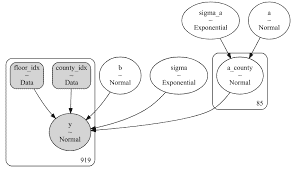
Multilevel models is a term used for models for data with hierarchical structure. The term is most commonly used in the social sciences. We can use the methodology we have already developed to fit some of these models.

We take as our example some data from the Junior School Project collected from primary (U.S. term is elementary) schools in inner London. The data is described in detail in Mortimore, Sammons, Stoll, Lewis, and Ecob (1988) and a subset is analyzed extensively in Goldstein (1995).

The variables in the data are the school, the class within the school (up to four), gender, social class of the father $(\mathrm{I}=1$; II $=2$; III nonmanual $=3$; III manual $=4$; IV=5; V=6; Long-term unemployed $=7$; Not currently employed=8; Father absent=9), raven’s test in year 1, student id number, english test score, mathematics test score and school year (coded 0,1 , and 2 for years one, two and three). So there are up to three measures per student. The data was obtained from the Multilevel Models project at http://www.ioe.ac.uk/multilevel/.

We shall take as our response the math test score result from the final year and try to model this as a function of gender, social class and the Raven’s test score from the first year which might be taken as a measure of ability when entering the school. We subset the data to ignore the math scores from the first two years:
$>\operatorname{data}(j s p)$
$>j \operatorname{spr}<-j \operatorname{sp} \quad[j \operatorname{sp} \$ y e a r==2$,
We start with two plots of the data. Due to the discreteness of the score results, it is helpful to jitter (add small random perturbations) the scores to avoid overprinting:

plot (jitter (math) jitter (raven), data=jspr, xlab=”Raven
score”,
$\quad$ ylab=”Math score”)
boxplot (math social, data=jspr,xlab=”Social
class”,ylab=”Math score”)
In Figure 8.4, we can see the positive correlation between the Raven’s test score and the final math score. The maximum math score was 40 which reduces the variability at the upper end of the scale. We also see how the math scores tend to decline with social class.

广义线性模型代考

统计代写|广义线性模型代写generalized linear model代考|Crossed Effects

当效果没有嵌套时，据说它们是交叉的。在全因子设计中，效应完全交叉，因为一个因素的每个水平都与另一个因素的每个水平发生。然而，在其他一些设计中，交叉是不完整的。即使在所有四个组合中只出现两个因素的两个水平，这些因素也会交叉。不完全交叉的一个例子是拉丁方设计，其中有一个处理因子和两个区组因子。尽管并非所有因素组合都会发生，但区组因素并不嵌套。当至少发生一些交叉时，不能使用嵌套设计的方法。我们考虑一个拉丁方的例子。

在 Davies (1954) 报告的一项实验中，四种材料 A、B、C 和 D 被送入磨损试验机。反应是体重减轻0.1 米米在测试期间。该机器一次可以处理四个样品，过去的经验表明这四个样品的位置存在一些差异。还怀疑运行与运行之间存在一些差异。可以在 Faraway (2004) 中找到该数据集的固定效应分析。进行了四次运行。可以观察到设计的拉丁方结构：

lmer 函数能够识别运行和位置效应交叉并适当地拟合模型。固定效应的 F 检验与相应的固定效应分析几乎相同。唯一的区别是固定效应分析使用的分母自由度为 6，而随机效应分析以估计的随机效应参数为条件，从而产生 12 个自由度。区别在这里并不重要。

随机效应的显着性可以使用参数引导方法进行测试。然而，由于该实验的设计已经限制了随机化以允许这些影响，因此没有动机进行这些测试，因为我们不会修改当前实验的分析。

固定效应分析在某种程度上更容易执行，但随机效应分析的优点是可以估计区组因子的变化，这在未来的研究中更有用。此实验的运行效果的固定效果估计仅对当前研究有用。

统计代写|广义线性模型代写generalized linear model代考|Multilevel Models

多级模型是用于具有层次结构的数据模型的术语。该术语在社会科学中最常用。我们可以使用我们已经开发的方法来拟合其中一些模型。
我们以初级学校项目的一些数据为例，这些数据是从伦敦市中心的小学（美国术语是小学）收集的。Mortimore、Sammons、Stoll、Lewis 和 Ecob (1988) 对数据进行了详细描述， Goldstein (1995) 对其中一个子集进行了广泛分析。
数据中的变量是学校，学校内的班级（最多四个），性别，父亲的社会阶层 $(\mathrm{I}=1 ; 二=2$; III 非手动 $=3$; 三、说明书 $=4 ; I \mathrm{I}=5 ； \mathrm{~V}=6$ ；长期失业 $=7$; 目前末就业 $=8$ ；父亲缺席 $=9 ）$ ，第一年的瑞文考试，学号，英语考试成绩，数学考试成绩和学年（第一，第二和第三年编码为 0,1 和 2) 。所以每个学生最多有 3 个小节。数据来自 http://www.ioe.ac.uk/multilevel/ 的多级模型项目。
我们应将最后一年的数学考试成绩作为我们的回应，并尝试将其建模为性别、社会阶层和第一年的 Raven 考试成绩的函数，这可能被视为入学时的能力衡量标准. 我们对数据进行子集化以忽略前两年的数学成绩:
$>\operatorname{data}(j s p)$
$>j$ spr $<-j$ sp $\quad[j$ sp $\$ y e a r==2$,
我们从两个数据图开始。由于分数结果的离散性，抖动（添加小的随机扰动) 分数有助于避免㨕印:
plot (jitter (math) jitter (raven), data=jspr, $x l a b=$ “Raven
分数”,
ylab=”Math score”)
boxplot (math social, data=jspr,xlab=”Social
class”,ylab=”Math score”)
在图8.4中，我们可以看到Raven的考试成绩和最终的数学成绩呈正相关关系. 最高数学分数为 40，这减少了量表上端的可变性。我们还看到数学成绩如何随着社会阶层的增加而下降。

统计代写|广义线性模型代写generalized linear model代考请认准statistics-lab™

统计代写请认准statistics-lab™. statistics-lab™为您的留学生涯保驾护航。

金融工程代写

金融工程是使用数学技术来解决金融问题。金融工程使用计算机科学、统计学、经济学和应用数学领域的工具和知识来解决当前的金融问题，以及设计新的和创新的金融产品。

非参数统计代写

非参数统计指的是一种统计方法，其中不假设数据来自于由少数参数决定的规定模型；这种模型的例子包括正态分布模型和线性回归模型。

广义线性模型代考

广义线性模型（GLM）归属统计学领域，是一种应用灵活的线性回归模型。该模型允许因变量的偏差分布有除了正态分布之外的其它分布。

术语广义线性模型（GLM）通常是指给定连续和/或分类预测因素的连续响应变量的常规线性回归模型。它包括多元线性回归，以及方差分析和方差分析（仅含固定效应）。

有限元方法代写

有限元方法（FEM）是一种流行的方法，用于数值解决工程和数学建模中出现的微分方程。典型的问题领域包括结构分析、传热、流体流动、质量运输和电磁势等传统领域。

有限元是一种通用的数值方法，用于解决两个或三个空间变量的偏微分方程（即一些边界值问题）。为了解决一个问题，有限元将一个大系统细分为更小、更简单的部分，称为有限元。这是通过在空间维度上的特定空间离散化来实现的，它是通过构建对象的网格来实现的：用于求解的数值域，它有有限数量的点。边界值问题的有限元方法表述最终导致一个代数方程组。该方法在域上对未知函数进行逼近。[1] 然后将模拟这些有限元的简单方程组合成一个更大的方程系统，以模拟整个问题。然后，有限元通过变化微积分使相关的误差函数最小化来逼近一个解决方案。

tatistics-lab作为专业的留学生服务机构，多年来已为美国、英国、加拿大、澳洲等留学热门地的学生提供专业的学术服务，包括但不限于Essay代写，Assignment代写，Dissertation代写，Report代写，小组作业代写，Proposal代写，Paper代写，Presentation代写，计算机作业代写，论文修改和润色，网课代做，exam代考等等。写作范围涵盖高中，本科，研究生等海外留学全阶段，辐射金融，经济学，会计学，审计学，管理学等全球99%专业科目。写作团队既有专业英语母语作者，也有海外名校硕博留学生，每位写作老师都拥有过硬的语言能力，专业的学科背景和学术写作经验。我们承诺100%原创，100%专业，100%准时，100%满意。

随机分析代写

随机微积分是数学的一个分支，对随机过程进行操作。它允许为随机过程的积分定义一个关于随机过程的一致的积分理论。这个领域是由日本数学家伊藤清在第二次世界大战期间创建并开始的。

时间序列分析代写

随机过程，是依赖于参数的一组随机变量的全体，参数通常是时间。随机变量是随机现象的数量表现，其时间序列是一组按照时间发生先后顺序进行排列的数据点序列。通常一组时间序列的时间间隔为一恒定值（如1秒，5分钟，12小时，7天，1年），因此时间序列可以作为离散时间数据进行分析处理。研究时间序列数据的意义在于现实中，往往需要研究某个事物其随时间发展变化的规律。这就需要通过研究该事物过去发展的历史记录，以得到其自身发展的规律。

回归分析代写

多元回归分析渐进（Multiple Regression Analysis Asymptotics）属于计量经济学领域，主要是一种数学上的统计分析方法，可以分析复杂情况下各影响因素的数学关系，在自然科学、社会和经济学等多个领域内应用广泛。

MATLAB代写

MATLAB 是一种用于技术计算的高性能语言。它将计算、可视化和编程集成在一个易于使用的环境中，其中问题和解决方案以熟悉的数学符号表示。典型用途包括：数学和计算算法开发建模、仿真和原型制作数据分析、探索和可视化科学和工程图形应用程序开发，包括图形用户界面构建MATLAB 是一个交互式系统，其基本数据元素是一个不需要维度的数组。这使您可以解决许多技术计算问题，尤其是那些具有矩阵和向量公式的问题，而只需用 C 或 Fortran 等标量非交互式语言编写程序所需的时间的一小部分。MATLAB 名称代表矩阵实验室。MATLAB 最初的编写目的是提供对由 LINPACK 和 EISPACK 项目开发的矩阵软件的轻松访问，这两个项目共同代表了矩阵计算软件的最新技术。MATLAB 经过多年的发展，得到了许多用户的投入。在大学环境中，它是数学、工程和科学入门和高级课程的标准教学工具。在工业领域，MATLAB 是高效研究、开发和分析的首选工具。MATLAB 具有一系列称为工具箱的特定于应用程序的解决方案。对于大多数 MATLAB 用户来说非常重要，工具箱允许您学习和应用专业技术。工具箱是 MATLAB 函数（M 文件）的综合集合，可扩展 MATLAB 环境以解决特定类别的问题。可用工具箱的领域包括信号处理、控制系统、神经网络、模糊逻辑、小波、仿真等。

R语言代写	问卷设计与分析代写
PYTHON代写	回归分析与线性模型代写
MATLAB代写	方差分析与试验设计代写
STATA代写	机器学习/统计学习代写
SPSS代写	计量经济学代写
EVIEWS代写	时间序列分析代写
EXCEL代写	深度学习代写
SQL代写	各种数据建模与可视化代写

统计代写|广义线性模型代写generalized linear model代考|MAST30025

Posted on 2023年2月11日2023年2月11日 by statistics-lab

如果你也在怎样代写广义线性模型generalized linear model这个学科遇到相关的难题，请随时右上角联系我们的24/7代写客服。

我们提供的广义线性模型generalized linear model及其相关学科的代写，服务范围广, 其中包括但不限于:

Statistical Inference 统计推断
Statistical Computing 统计计算
Advanced Probability Theory 高等概率论
Advanced Mathematical Statistics 高等数理统计学
(Generalized) Linear Models 广义线性模型
Statistical Machine Learning 统计机器学习
Longitudinal Data Analysis 纵向数据分析
Foundations of Data Science 数据科学基础

统计代写|广义线性模型代写generalized linear model代考|MAST30025

统计代写|广义线性模型代写generalized linear model代考|Split Plots

Split plot designs originated in agriculture, but occur frequently in other settings. As the name implies, main plots are split into several subplots. The main plot is treated with a level of one factor while the levels of some other factor are allowed to vary with the subplots. The design arises as a result of restrictions on a full randomization. For example, a field may be divided into four subplots. It may be possible to plant different varieties in the subplots, but only one type of irrigation may be used for the whole field. Note the distinction between split plots and blocks. Blocks are features of the experimental units which we have the option to take advantage of in the experimental design. Split plots impose restrictions on what assignments of factors are possible. They impose requirements on the design that prevent a complete randomization. Split plots often arise in nonagricultural settings when one factor is easy to change while another factor takes much more time to change. If the experimenter must do all runs for each level of the hard-to-change factor consecutively, a split-plot design results with the hardto-change factor representing the whole plot factor.

Consider the following example. In an agricultural field trial, the objective was to determine the effects of two crop varieties and four different irrigation methods. Eight fields were available, but only one type of irrigation may be applied to each field. The fields may be divided into two parts with a different variety planted in each half. The whole plot factor is the method of irrigation, which should be randomly assigned to the fields. Within each field, the variety is randomly assigned. Here is a summary of the data:

The irrigation and variety are fixed effects, but the field is clearly a random effect. We must also consider the interaction between field and variety, which is necessarily also a random effect because one of the two components is random. The fullest model that we might consider is:
$$
y_{i j k}=\mu+i_i+v_j+(\mathrm{iv}){i j}+f_k+(\mathrm{v} f){j k}+\varepsilon_{i j k}
$$
$\mu, i_i, v_j,(i v){i j}$ are fixed effects, the rest are random having variances $\sigma_f^2, \sigma{v f}^2$ and $\sigma_{\varepsilon}^2 \cdot$ Note that we have no $(i f)_{i k}$ term in this model. It would not be possible to estimate such an effect since only one type of irrigation is used on a given field; the factors are not crossed.

统计代写|广义线性模型代写generalized linear model代考|Nested Effects

When the levels of one factor vary only within the levels of another factor, that factor is said to be nested. For example, when measuring the performance of workers at several different job locations, if the workers only work at one location, the workers are nested within the locations. If the workers work at more than one location, then the workers are crossed with locations.

Here is an example to illustrate nesting. Consistency between laboratory tests is important and yet the results may depend on who did the test and where the test was performed. In an experiment to test levels of consistency, a large jar of dried egg powder was divided up into a number of samples. Because the powder was homogenized, the fat content of the samples is the same, but this fact is withheld from the laboratories. Four samples were sent to each of six laboratories. Two of the samples were labeled as $\mathrm{G}$ and two as $\mathrm{H}$, although in fact they were identical. The laboratories were instructed to give two samples to two different technicians. The technicians were then instructed to divide their samples into two parts and measure the fat content of each. So each laboratory reported eight measures, each technician four measures, that is, two replicated measures on each of two samples. The data comes from Bliss (1967): Although the technicians have been labeled “one” and “two,” they are two different people in each lab. Thus the technician factor is nested within laboratories. Furthermore, even though the samples are labeled”H” and “G,” these are not the same samples across the technicians and the laboratories. Hence we have samples nested within technicians. Technicians and samples should be treated as random effects since we may consider these as randomly sampled. If the labs were specifically selected, then they should be taken a fixed effects. If, however, they were randomly selected from those available, then they should be treated as random effects. If the purpose of the study is come to some conclusion about consistency across laboratories, the latter approach is advisable.

广义线性模型代考

统计代写|广义线性模型代写generalized linear model代考|Split Plots

裂区设计起源于农业，但在其他环境中也经常出现。顾名思义，主要情节被分成几个次要情节。主要地块用一个因素的水平处理，而其他一些因素的水平允许随子地块变化。该设计是由于对完全随机化的限制而产生的。例如，一个田地可以被分成四个子地块。可以在子地块中种植不同的品种，但整个田地只能使用一种灌溉方式。注意裂区和块之间的区别。块是实验单元的特征，我们可以选择在实验设计中利用这些特征。裂区对可能的因子分配施加了限制。他们对防止完全随机化的设计提出要求。当一个因素很容易改变而另一个因素需要更多时间才能改变时，裂区通常出现在非农业环境中。如果实验者必须连续地对难以更改的因子的每个水平进行所有试验，则裂区设计会产生一个裂区设计，其中难以更改的因子代表整区因子。
考虑以下示例。在农业田间试验中，目标是确定两种作物品种和四种不同灌溉方法的影响。有八块田地，但每块田地只能采用一种淮溉方式。这些田地可以分成两部分，每半部分种植不同的品种。整区因子是灌溉方式，应随机分配到田间。在每个字段中，品种是随机分配的。以下是数据樀要:
灌溉和品种是固定效应，但田地显然是随机效应。我们还必须考虑领域和多样性之间的相互作用，这也必然是一种随机效应，因为这两个成分之一是随机的。我们可能考虑的最完整的模型是:
$$
y_{i j k}=\mu+i_i+v_j+(\mathrm{iv}) i j+f_k+(\mathrm{v} f) j k+\varepsilon_{i j k}
$$
$\mu, i_i, v_j,(i v) i j$ 是固定效应，其余是随机的，有方差 $\sigma_f^2, \sigma v f^2$ 和 $\sigma_{\varepsilon}^2$ 请注意，我们没有 $(\text { if })_{i k}$ 这个模型中的术语。不可能估计这种影响，因为给定的田地只使用一种濩溉方式；这些因素没有交叉。

统计代写|广义线性模型代写generalized linear model代考|Nested Effects

当一个因素的水平仅在另一个因素的水平内变化时，该因素被称为嵌套。例如，在衡量多个不同工作地点的员工的绩效时，如果员工只在一个地点工作，则这些员工会嵌套在这些地点内。如果工人在不止一个地点工作，那么这些工人会跨地点工作。

下面是一个例子来说明嵌套。实验室测试之间的一致性很重要，但结果可能取决于谁进行了测试以及在何处进行测试。在测试一致性水平的实验中，将一大罐干蛋粉分成许多样品。由于粉末经过均质化处理，因此样品的脂肪含量相同，但实验室隐瞒了这一事实。四个样本被送到六个实验室中的每一个。其中两个样本被标记为G和两个作为H，尽管实际上它们是相同的。指示实验室将两个样本提供给两名不同的技术人员。然后指示技术人员将他们的样品分成两部分并测量每部分的脂肪含量。因此，每个实验室报告了八项措施，每位技术人员报告了四项措施，即对两个样品中的每一个样品进行了两次重复测量。数据来自 Bliss (1967)：虽然技术人员被标记为“一个”和“两个”，但他们在每个实验室中都是两个不同的人。因此，技术因素嵌套在实验室中。此外，即使样本被标记为“H”和“G”，但这些样本在技术人员和实验室中并不是相同的。因此，我们将样本嵌套在技术人员中。技术人员和样本应被视为随机效应，因为我们可以将它们视为随机抽样。如果专门选择实验室，则应采用固定效果。但是，如果它们是从可用的那些中随机选择的，那么它们应该被视为随机效应。如果研究的目的是得出关于实验室间一致性的结论，则后一种方法是可取的。

统计代写请认准statistics-lab™. statistics-lab™为您的留学生涯保驾护航。

金融工程代写

非参数统计代写

非参数统计指的是一种统计方法，其中不假设数据来自于由少数参数决定的规定模型；这种模型的例子包括正态分布模型和线性回归模型。

广义线性模型代考

广义线性模型（GLM）归属统计学领域，是一种应用灵活的线性回归模型。该模型允许因变量的偏差分布有除了正态分布之外的其它分布。

有限元方法代写

随机分析代写

时间序列分析代写

回归分析代写

MATLAB代写

R语言代写	问卷设计与分析代写
PYTHON代写	回归分析与线性模型代写
MATLAB代写	方差分析与试验设计代写
STATA代写	机器学习/统计学习代写
SPSS代写	计量经济学代写
EVIEWS代写	时间序列分析代写
EXCEL代写	深度学习代写
SQL代写	各种数据建模与可视化代写

统计代写|广义线性模型代写generalized linear model代考|STATS3001

Posted on 2023年2月10日2023年2月10日 by statistics-lab

如果你也在怎样代写广义线性模型generalized linear model这个学科遇到相关的难题，请随时右上角联系我们的24/7代写客服。

我们提供的广义线性模型generalized linear model及其相关学科的代写，服务范围广, 其中包括但不限于:

Statistical Inference 统计推断
Statistical Computing 统计计算
Advanced Probability Theory 高等概率论
Advanced Mathematical Statistics 高等数理统计学
(Generalized) Linear Models 广义线性模型
Statistical Machine Learning 统计机器学习
Longitudinal Data Analysis 纵向数据分析
Foundations of Data Science 数据科学基础

统计代写|广义线性模型代写generalized linear model代考|STATS3001

统计代写|广义线性模型代写generalized linear model代考|Choice of Link Function

We must choose a link function to specify a binomial regression model. It is usually not possible to make this choice based on the data alone. For regions of moderate $p$, that is not close to zero or one, the link functions we have proposed are quite similar and so a very large amount of data would be necessary to distinguish between them. Larger differences are apparent in the tails, but for very small $p$, one needs a very large amount of data to obtain just a few successes, making it expensive to distinguish between link functions in this region. So usually, the choice of link function is made based on assumptions derived from physical knowledge or simple convenience. We now look at some of the advantages and disadvantages of the three proposed link functions and what motivates the choice.

Bliss (1935) analyzed some data on the numbers of insects dying at different levels of insecticide concentration. We fit all three link functions:

The lines in the left panel of Figure $2.3$ do not seem very different, but look at the relative differences:
$>$ matplot $(x$, cbind $(p p / p l,(1-p p) /(1-$
pl)), type=”1″, $x l a b=$ Dose”, $1 \mathrm{ab}=$ “Ratio”)
$>$ matplot (x, cbind (pc/pl, (1-pc) /(1-
pl)), type=”1″, 1 lab=”Dose”,ylab=”Ratio”)
as they appear in the second and third panels of Figure 2.3. We see that the probit and logit differ substantially in the tails. The same phenomenon is observed for the complementary log-log. This is problematic since the former plot indicates it would be difficult to distinguish between the two using the data we have. This is an issue in trials of potential carcinogens and other substances that must be tested for possible harmful effects on humans. Some substances are highly poisonous in that their effects become immediately obvious at doses that might normally be experienced in the environment. It is not difficult to detect such substances. However, there are other substances whose harmful effects only become apparent at large dosages where the observed probabilities are sufficiently larger than zero to become estimable without immense sample sizes. In order to estimate the probability of a harmful effect at a low dose, it would be necessary to select an appropriate link function and yet the data for high dosages will be of little help in doing this. As Paracelsus (1493-1541) said, “All substances are poisons; there is none which is not a poison. The right dose differentiates a poison.”

A good example of this problem is asbestos. Information regarding the harmful effects of asbestos derives from historical studies of workers in industries exposed to very high levels of asbestos dust. However, we would like to know the risk to individuals exposed to low levels of asbestos dust such as those found in old buildings. It is virtually impossible to accurately determine this risk. We cannot accurately measure exposure or outcome. This is not to argue that nothing should be done, but that decisions should be made in recognition of the uncertainties.

统计代写|广义线性模型代写generalized linear model代考|Goodness of Fit

The deviance is one measure of how well the model fits the data, but there are alternatives. The Pearson’s $X^2$ statistic takes the general form:
$$
X^2=\sum_{i=1}^n \frac{\left(O_i-E_i\right)^2}{E_i}
$$
where $O_i$ is the observed counts and $E_i$ are the expected counts for case $i$. For a binomial response, we count the number of successes for which $\theta_i=y_i$ while $E_i=n_i \hat{p}i$ and failures for which $O_i=n_i-y_i$ and $E_i=n_i\left(1-\hat{p}_i\right){\text {which results in: }}$
$$
X^2=\sum_{i=1}^n \frac{\left(y_i-n_i \hat{p}i\right)^2}{n_i \hat{p}_i\left(1-\hat{p}_i\right)} $$ If we define Pearson residuals as: $$ r_i^P=\left(y_i-n_i \hat{p}_i\right) / \sqrt{\operatorname{var} \hat{y}_i} $$ which can be viewed as a type of standardized residual, then $X^2=\sum{i=1}^n\left(r_i^P\right)^2$.So the Pearson’s $X^2$ is analogous to the residual sum of squares used in normal linear models.
The Pearson $X^2$ will typically be close in size to the deviance and can be used in the same manner. Alternative versions of the hypothesis tests described above might use the $X^2$ in place of the deviance with the same approximate null distributions.

However, some care is necessary because the model is fit to minimize the deviance and not the Pearson’s $X^2$. This means that it is possible, although unlikely, that the $X^2$ could increase as a predictor is added to the model. $X^2$ can be computed like this:

The proportion of variance explained or $R^2$ is a popular measure of fit for normal linear models. We might consider applying the same concept to binomial regression models by using the proportion of deviance explained. However, a better statistic is due to Naglekerke (1991):
$$
R^2=\frac{1-\left(\hat{L}0 / \hat{L}\right)^{2 / n}}{1-\hat{L}_o^{2 / n}}=\frac{1-\exp \left(\left(D-D{\text {null }}\right) / n\right)}{1-\exp \left(-D_{\text {null }} / n\right)}
$$

广义线性模型代考

统计代写|广义线性模型代写generalized linear model代考|Choice of Link Function

我们必须选择一个链接函数来指定二项式回归模型。通常不可能仅根据数据做出这种选择。对于中度地区 $p$ ，即不接近于零或一，我们提出的链接函数非常相似，因此需要大量数据来区分它们。较大的差异在尾部很明显，但对于非常小的 $p$ ，需要大量数据才能获得少数成功，因此区分该区域中的链㢺功能非常昂贵。所以通常，链㢺函数的选择是基于从物理知识或简单的便利性得出的假设。我们现在看一下所提出的三个链接函数的一些优点和缺点，以及选择的动机。

Bliss (1935) 分析了一些关于在不同杀虫剂浓度水平下死亡的昆蝼量的数据。我们适合所有三个链㢺功能:
图左面板中的线条 $2.3$ 看起来差别不大，但是看看相对的区别:
$>$ 绘图 $(x$, 绑定 $(p p / p l,(1-p p) /(1-$
pl)), type=”1″, $x l a b=$ 剂量”, $1 \mathrm{ab}=$ “比率”)
$>$ matplot $(x$, cbind $(\mathrm{pc} / \mathrm{pl},(1-\mathrm{pc}) /(1-$
pl)), type=”1″, 1 lab=”Dose”,ylab=”Ratio”)
它们出现在图 $2.3$ 的第二和第三图中。我们看到 probit 和 logit 在尾部有很大不同。互补对数对数也观察到相同的现象。这是有问题的，因为前一个图表明很难使用我们拥有的数据来区分两者。这是潜在致癌物和其他必须测试对人体可能有害影响的物质试验中的一个问题。有些物质具有剧毒，因为它们的影响在正常情况下可能在环境中经历的剂量下立即显现出来。检则此类物质并不困难。然而，还有其他一些物质，其有害影响只有在大剂量时才会显现，在这种情况下，观察到的概率远大于零，无需大量样本即可估计。为了估计低剂量有害影响的可能性，有必要选择一个合适的链接函数，但高剂量的数据对此帮助不大。正如 Paracelsus (14931541) 所兑，“所有物质都是毒药; 无一不是毒。正确的剂量可以区分毒药。”
这个问题的一个很好的例子是石棉。有关石棉有害影响的信息来自对暴露于高浓度石棉粉尘的行业工人的历史研究。但是，我们想知道暴露于低浓度石棉粉尘（例如在旧建筑物中发现的石棉粉尘）的个人所面临的风险。准确确定这种风险几乎是不可能的。我们无法准确衡量风险或结果。这并不是说什么都不应该做，而是应该在认识到不确定性的情兄下做出决定。

统计代写|广义线性模型代写generalized linear model代考|Goodness of Fit

偏差是模型与数据拟合程度的一种衡量标准，但还有其他选择。皮尔逊的 $X^2$ 统计采用一般形式:
$$
X^2=\sum_{i=1}^n \frac{\left(O_i-E_i\right)^2}{E_i}
$$
在哪里 $O_i$ 是观察到的计数和 $E_i$ 是案例的预期计数 $i$. 对于二项式响应，我们计算成功的次数 $\theta_i=y_i$ 尽管 $E_i=n_i \hat{p} i$ 和失败的原因 $O_i=n_i-y_i$ 和 $E_i=n_i\left(1-\hat{p}i\right)$ which results in: $$ X^2=\sum{i=1}^n \frac{\left(y_i-n_i \hat{p} i\right)^2}{n_i \hat{p}i\left(1-\hat{p}_i\right)} $$ 如果我们将 Pearson 残差定义为: $$ r_i^P=\left(y_i-n_i \hat{p}_i\right) / \sqrt{\operatorname{var} \hat{y}_i} $$ 可以看作是一种标准化残差，那么 $X^2=\sum i=1^n\left(r_i^P\right)^2$. 所以皮尔逊的 $X^2$ 类似于正态线性模型中使用的残差平方和。皮尔逊 $X^2$ 通常在大小上接近偏差，并且可以以相同的方式使用。上述假设检验的替代版本可能使用 $X^2$ 用相同的近似零分布代替偏差。但是，有些注意是必要的，因为该模型适用于最小化偏差而不是 Pearson 的 $X^2$. 这意味着尽管不太可能，但有可能 $X^2$ 可能会随着预测变量添加到模型中而增加。 $X^2$ 可以这样计算: 解释的方差比例或 $R^2$ 是正态线性模型的一种流行的拟合度量。我们可能会考虑通过使用解释的偏差比例将相同的概念应用于二项式回归模型。然而，更好的统计数据来自 Naglekerke (1991): $$ R^2=\frac{1-(\hat{L} 0 / \hat{L})^{2 / n}}{1-\hat{L}_o^{2 / n}}=\frac{1-\exp ((D-D \text { null }) / n)}{1-\exp \left(-D{\text {null }} / n\right)}
$$

统计代写请认准statistics-lab™. statistics-lab™为您的留学生涯保驾护航。

金融工程代写

非参数统计代写

非参数统计指的是一种统计方法，其中不假设数据来自于由少数参数决定的规定模型；这种模型的例子包括正态分布模型和线性回归模型。

广义线性模型代考

广义线性模型（GLM）归属统计学领域，是一种应用灵活的线性回归模型。该模型允许因变量的偏差分布有除了正态分布之外的其它分布。

有限元方法代写

随机分析代写

时间序列分析代写

回归分析代写

MATLAB代写

R语言代写	问卷设计与分析代写
PYTHON代写	回归分析与线性模型代写
MATLAB代写	方差分析与试验设计代写
STATA代写	机器学习/统计学习代写
SPSS代写	计量经济学代写
EVIEWS代写	时间序列分析代写
EXCEL代写	深度学习代写
SQL代写	各种数据建模与可视化代写

统计代写|广义线性模型代写generalized linear model代考|STAT7608

Posted on 2023年2月10日2023年2月10日 by statistics-lab

如果你也在怎样代写广义线性模型generalized linear model这个学科遇到相关的难题，请随时右上角联系我们的24/7代写客服。

我们提供的广义线性模型generalized linear model及其相关学科的代写，服务范围广, 其中包括但不限于:

Statistical Inference 统计推断
Statistical Computing 统计计算
Advanced Probability Theory 高等概率论
Advanced Mathematical Statistics 高等数理统计学
(Generalized) Linear Models 广义线性模型
Statistical Machine Learning 统计机器学习
Longitudinal Data Analysis 纵向数据分析
Foundations of Data Science 数据科学基础

统计代写|广义线性模型代写generalized linear model代考|STAT7608

统计代写|广义线性模型代写generalized linear model代考|Interpreting Odds

Odds are sometimes a better scale than probability to represent chance. They arose as a way to express the payoffs for bets. An evens bet means that the winner gets paid an equal amount to that staked. A $3-1$ against bet would pay $\$ 3$ for every $\$ 1$ bet while a $3-1$ on bet would pay only $\$ 1$ for every $\$ 3$ bet. If these bets are fair in the sense that a bettor would break even in the long-run average, then we can make a correspondence to probability. Let $p$ be the probability and $o$ be the odds, where we represent $3-1$ against as $1 / 3$ and $3-1$ on as 3 , then the following relationships hold:
$$
\frac{p}{1-p}=o \quad p=\frac{o}{1+o}
$$
One mathematical advantage of odds is that they are unbounded above which makes them more convenient for some modeling purposes.

Odds also form the basis of a subjective assessment of probability. Some probabilities are determined from considerations of symmetry or long-term frequencies, but such information is often unavailable. Individuals may determine their subjective probability for events by considering what odds they would be prepared to offer on the outcome. Under this theory, other potential persons would be allowed to place bets for or against the event occurring. Thus the individual would be forced to make an honest assessment of probability to avoid financial loss.
If we have two covariates $x_1$ and $x_2$, then the logistic regression model is:
$$
\log (o \mathrm{ods})=\log \left(\frac{p}{1-p}\right)=\beta_0+\beta_1 x_1+\beta_2 x_2
$$

Now $\beta_1$ can be interpreted as follows: a unit increase in $x_1$ with $x_2$ held fixed increases the log-odds of success by $\beta_1$ or increases the odds of success by a factor of exp $\beta_1$. Of course, the usual interpretational difficulties regarding causation apply as in standard regression. No such simple interpretation exists for other links such as the probit.

An alternative notion to odds-ratio is relative risk. Suppose the probability of “success” in the presence of some condition is $p_1$ and $p_2$ in its absence. The relative risk is $P_1 / P_2$. For rare outcomes, the relative risk and the o dds ratio will be very similar, but for larger probabilities, there may be substantial differences. There is some debate over which is the more intuitive way of expressing the effect of some condition.

统计代写|广义线性模型代写generalized linear model代考|Prospective and Retrospective Sampling

In prospective sampling, the predictors are fixed and then the outcome is observed. In other words, in the infant respiratory disease example shown in Table 2.1, we would select a sample of newborn girls and boys whose parents had chosen a particular method of feeding and then monitor them for their first year. This is also called a cohort study.
In retrospective sampling, the outcome is fixed and then the predictors are observed. Typically, we would find infants coming to a doctor with a respiratory disease in the first year and then record their sex and method of feeding. We would also obtain a sample of respiratory disease-free infants and record their information. How these samples are obtained is important-we require that the probability of inclusion in the study is independent of the predictor values. This is also called a case-control study.

Since the question of interest is how the predictors affect the response, prospective sampling seems to be required. Let’s focus on just boys who are breast or bottle fed. The data we need is:

Given the infant is breast fed, the log-odds of having a respiratory disease are $\log 47 / 447=-2.25$
Given the infant is bottle fed, the log-odds of having a respiratory disease are log $77 / 381=-1.60$
The difference between these two log-odds, $\Delta=-1.60–2.25=0.65$, represents the increased risk of respiratory disease incurred by bottle feeding relative to breast feeding. This is the log-odds ratio.

广义线性模型代考

统计代写|广义线性模型代写generalized linear model代考|Interpreting Odds

赔率有时比概率更能代表机会。它们的出现是作为一种表达投注收益的方式。均等投注意味着获胜者将获得与下注金额相等的报酬。 $A 3-1$ 反对赌注会付出代价 $\$ 3$ 每一个 $\$ 1$ 下注 $3-1$ 打赌只会支付 $\$ 1$ 每一个 $\$ 3$ 赌注。如果这些投注在投注者长期平均收支平衡的意义上是公平的，那么我们可以与概率对应。让 $p$ 是概率和 $o$ 成为赔率，我们代表的地方 $3-1$ 反对作为 $1 / 3$ 和 $3-1$ 作为 3 ，则以下关系成立:
$$
\frac{p}{1-p}=o \quad p=\frac{o}{1+o}
$$
赔率的一个数学优势是它们不受限制，这使得它们更便于某些建模目的。
赔率也是概率主观评估的基础。一些概率是根据对称性或长期频率的考虑来确定的，但此类信息通常无法获得。个人可以通过考虑他们愿意为结果提供多少赔率来确定他们对事件的主观概率。根据这一理论，其他潜在的人将被允许为或反对正在发生的事件下注。因此，个人将被迫对概率做出诚实的评估，以避免经济损失。如果我们有两个协变量 $x_1$ 和 $x_2$ ，则逻辑回归模型为:
$$
\log (\text { oods })=\log \left(\frac{p}{1-p}\right)=\beta_0+\beta_1 x_1+\beta_2 x_2
$$
现在 $\beta_1$ 可以解释如下: 单位增加 $x_1$ 和 $x_2$ 保持固定增加了成功的对数几率 $\beta_1$ 或将成功几率增加 exp 倍 $\beta_1$. 当然，关于因果关系的常见解释困难适用于标准回归。其他链接 (例如 probit) 不存在这种简单的解释。
比值比的另一种概念是相对风险。假设在某些条件下“成功”的概率是 $p_1$ 和 $p_2$ 在没有它的情况下。相对风险是 $P_1 / P_2$. 对于罕见的结果，相对风险和优势比将非常相似，但对于更大的概率，可能会有很大差异。关于哪种是表达某些条件的影响的更直观的方式存在一些争论。

统计代写|广义线性模型代写generalized linear model代考|Prospective and Retrospective Sampling

在前瞻性抽样中，预恻变量是固定的，然后观察结果。换句话说，在表 $2.1$ 所示的婴儿呼吸系统疾病示例中，我们将选译父母选择特定喂养方法的新生儿女孩和男孩样本，然后在第一年监测他们。这也称为队列研究。
在回顾性抽样中，结果是固定的，然后观察预财因子。通常，我们会发现婴儿在第一年因呼吸系统疾病去看医生，然后记录他们的性别和喂养方式。我们还将获得无呼吸道疾病婴儿的样本并记录他们的信息。如何获得这些样本很重要一一我们要求纳入研究的概率与预则值无关。这也称为病例对岹研究。
由于感兴趣的问题是预测变量如何影响响应，因此似乎需要前瞻性抽样。让我们只关注母乳喂养或奶瓶喂养的男孩。我们需要的数据是:

鉴于婴儿是母乳喂养，患呼吸系统疾病的对数几率是 $\log 47 / 447=-2.25$
鉴于婴儿是奶瓶喂养，患呼吸系统疾病的对数几率是对数 $77 / 381=-1.60$ 这两个对数赔率之间的差异， $\Delta=-1.60-2.25=0.65$, 表示相对于母乳喂养，奶瓶喂养引起呼吸道疾病的风险增加。这是对数优势比。

统计代写请认准statistics-lab™. statistics-lab™为您的留学生涯保驾护航。

金融工程代写

非参数统计代写

非参数统计指的是一种统计方法，其中不假设数据来自于由少数参数决定的规定模型；这种模型的例子包括正态分布模型和线性回归模型。

广义线性模型代考

广义线性模型（GLM）归属统计学领域，是一种应用灵活的线性回归模型。该模型允许因变量的偏差分布有除了正态分布之外的其它分布。

有限元方法代写

随机分析代写

时间序列分析代写

回归分析代写

MATLAB代写

R语言代写	问卷设计与分析代写
PYTHON代写	回归分析与线性模型代写
MATLAB代写	方差分析与试验设计代写
STATA代写	机器学习/统计学习代写
SPSS代写	计量经济学代写
EVIEWS代写	时间序列分析代写
EXCEL代写	深度学习代写
SQL代写	各种数据建模与可视化代写

统计代写|广义线性模型代写generalized linear model代考|MAST30025

Posted on 2023年2月10日2023年2月10日 by statistics-lab

如果你也在怎样代写广义线性模型generalized linear model这个学科遇到相关的难题，请随时右上角联系我们的24/7代写客服。

我们提供的广义线性模型generalized linear model及其相关学科的代写，服务范围广, 其中包括但不限于:

Statistical Inference 统计推断
Statistical Computing 统计计算
Advanced Probability Theory 高等概率论
Advanced Mathematical Statistics 高等数理统计学
(Generalized) Linear Models 广义线性模型
Statistical Machine Learning 统计机器学习
Longitudinal Data Analysis 纵向数据分析
Foundations of Data Science 数据科学基础

统计代写|广义线性模型代写generalized linear model代考|Challenger Disaster Example

In January 1986, the space shuttle Challenger exploded shortly after launch. An investigation was launched into the cause of the crash and attention focused on the rubber O-ring seals in the rocket boosters. At lower temperatures, rubber becomes more brittle and is a less effective sealant. At the time of the launch, the temperature was $31^{\circ} \mathrm{F}$. Could the failure of the O-rings have been predicted? In the 23 previous shuttle missions for which data exists, some evidence of damage due to blow by and erosion was recorded on some O-rings. Each shuttle had two boosters, each with three O-rings. For each mission, we know the number of $\mathrm{O}$-rings out of six showing some damage and the launch temperature. This is a simplification of the problem-see Dalal, Fowlkes, and Hoadley (1989) for more details.

Let’s start our analysis with R. For help in obtaining R and installing the necessary add-on packages and datasets, please see Appendix B. First we load the data. To do this, you will first need to load the faraway package using the library command as seen in here. You will need to do this in every session that you run examples from this book. If you forget, you will receive a warning message about the data not being found. We then plot the proportion of damaged O-rings against temperature in Figure 2.1:
$>$ library (faraway)
$>$ data (orings)
$>$ plot (damage/ $6 \sim$ temp, orings, $x l i m=c(25,85)$, ylim $=$
$c(0,1)$,
$\quad x l a b=$ “Temperature”, ylab=”Prob of damage”)
We are interested in how the probability of failure in a given O-ring is related to the launch temperature and predicting that probability when the temperature is $31^{\circ} \mathrm{F}$. A naive approach, based on linear models, simply fits a line to this data:
$$
\begin{aligned}
& >\text { lmod }<-1 \mathrm{~lm} \text { (damage } / 6 \sim \text { temp, orings) } \\ & >\text { abline (lmod) }
\end{aligned}
$$
The fit is shown in Figure 2.1. There are several problems with this approach. Most obviously from the plot, it can predict probabilities greater than one or less than zero. One might suggest truncating predictions outside the range to zero or one as appropriate, but it does not seem eredible that these probabilities would be exactly zero or one, in this particular example or many others.

统计代写|广义线性模型代写generalized linear model代考|Binomial Regression Model

Suppose the response variable $Y_i$ for $i=1, \ldots, n_i$ is binomially distributed $B\left(n_i, p_i\right)$ so that:
$$
P\left(Y_i=y_i\right)=\left(\begin{array}{c}
n_i \
y_i
\end{array}\right) p_i^{y_i}\left(1-p_i\right)^{n_i-y_i}
$$
We further assume that the $Y_i$ are independent. The individual trials that compose the response $Y_i$ are all subject to the same $q$ predictors $\left(x_{i 1}, \ldots, x_{i q}\right)$. The group of trials is known as a covariate class. We need a model that describes the relationship of $x_1, \ldots, x_q$ to $p$. Following the linear model approach, we construct a linear predictor:
$$
\eta_i=\beta_0+\beta_1 x_{i 1}+\ldots+\beta_q x_{i q}
$$

Since the linear predictor can accommodate quantitative and qualitative predictors with the use of dummy variables and also allows for transformations and combinations of the original predictors, it is very flexible and yet retains interpretability. This notion that we can express the effect of the predictors on the response solely through the linear predictor is important. The idea can be extended to models for other types of response and is one of the defining features of the wider class of generalized linear models (GLMs) discussed in Chapter 6.

We have already seen above that setting $\eta_i=p_i$ is not appropriate because we require $0 \leq p_i \leq 1$. Instead we shall use a link function $g$ such that $\eta i=g\left(p_i\right)$. For this application, we shall need $g$ to be monotone and be such that $0 \leq \mathrm{g}^{-1}(\eta) \leq 1$ for any $\eta$. There are three common choices:

Logit: $\eta=\log (p /(1-p))$.
Probit: $\eta=\Phi^{-1}(p)$ where $\Phi^{-1}$ is the inverse normal cumulative distribution function.
Complementary $\log -\log : \eta=\log (-\log (1-p))$.
The idea of the link function is also one of the central ideas of generalized linear models. It is used to link the linear predictor to the mean of the response in the wider class of models.

We will compare these three choices of link function later, but first we estimate the parameters of the model. We shall use the method of maximum likelihood; see Appendix A for a brief introduction to this method. The log-likelihood is given by:
$$
l(\beta)=\sum_{i=1}^n\left[y_i \eta_i-n_i \log \left(1+e_i^\eta\right)+\log \left(\begin{array}{l}
n_i \
y_i
\end{array}\right)\right]
$$
We can maximize this to obtain the maximum likelihood estimates $\hat{\beta}$ and use the standard theory to obtain approximate standard errors. An algorithm to perform the maximization will be discussed in Chapter 6 .

广义线性模型代考

统计代写|广义线性模型代写generalized linear model代考|Challenger Disaster Example

1986 年 1 月，挑战者号航天飞机在发射后不久就爆炸了。对坠机原因展开了调查，并将注意力集中在火箭助推器中的橡胶 $O$ 形密封圈上。在较低的温度下，橡胶变得更脆并且是一种效果较差的密封剂。发射时的温度是 $31^{\circ} \mathrm{F}$. 是否可以预测 $\mathrm{O}$ 形圈的失效? 在现有数据的 23 次航天飞机任务中，一些 $O$ 形环上记录了由于吹过和侵蚀造成的损坏证据。每架航天飞机都有两个助推器，每个助推器都有三个 $O$ 形圈。对于每个任务，我们知道有多少 0 -六分之一的环显示了一些损坏和发射温度。这是问题的简化一一有关详细信息，请参阅 Dalal、Fowlkes 和 Hoadley (1989)。
让我们从 R 开始分析。有关获取 R和安装必要的附加包和数据集的帮助，请参阅附录 $B$ 。首先我们加载数据。为此，您首先需要使用此处所示的库命令加载 faraway 包。您将需要在运行本书示例的每个会话中执行此操作。如果您忘记了，您将收到有关末找到数据的警告消息。然后，我们在图 $2.1$ 中绘制损坏的 O 形圈与温度的比例:
$>$ 图书馆 (遥远)

数据 (orings)
$>$ 情节 (伤害 $6 \sim$ 温度, orings, $x$ lim $=c(25,85)$ ，优越的 $=$ $c(0,1)$,
$x l a b=$ “Temperature”, ylab=”Prob of damage”)
我们感兴趣的是给定 $O$ 形环的失效概率与发射温度的关系，并预测当温度为 $31^{\circ} \mathrm{F}$.一种基于线生模型的朴素方法只是为该数据拟合一条线:
$$
\begin{aligned}
& >\operatorname{lmod}<-1 \operatorname{lm}(\text { damage } / 6 \sim \text { temp, orings) } \\ & >\text { abline }(\operatorname{lmod})
\end{aligned}
$$
拟合如图 $2.1$ 所示。这种方法有几个问题。从图中最明显的是，它可以预测大于一或小于零的概率。有人可能会建议适当地将范围外的预测截断为零或一，但在这个特定示例或许多其他示例中，这些概率恰好为零或一似乎并不可信。

统计代写|广义线性模型代写generalized linear model代考|Binomial Regression Model

假设响应变量 $Y_i$ 为了 $i=1, \ldots, n_i$ 是二项分布的 $B\left(n_i, p_i\right)$ 以便:
$$
P\left(Y_i=y_i\right)=\left(n_i y_i\right) p_i^{y_i}\left(1-p_i\right)^{n_i-y_i}
$$
我们进一步假设 $Y_i$ 是独立的。构成响应的个别试验 $Y_i$ 都受到相同的 $q$ 预测器 $\left(x_{i 1}, \ldots, x_{i q}\right)$. 这组试验称为协变量类。我们需要一个描述关系的模型 $x_1, \ldots, x_q$ 到 $p$. 按照线性模型方法，我们构建了一个线性预测器:
$$
\eta_i=\beta_0+\beta_1 x_{i 1}+\ldots+\beta_q x_{i q}
$$
由于线生预测器可以通过使用虚拟变量来容纳定量和定性预测器，并且还允许原始预测器的转换和组合，因此它非常灵活并保留了可解释性。我们可以仅通过线性预恻变量来表达预则变量对响应的影响这一概念很重要。这个想法可以扩展到其他类型吅应的模型，并且是第 6 章中讨论的更广泛的广义线性模型 (GLM) 类别的定义特征之一。
我们已经在上面看到了那个设置 $\eta_i=p_i$ 不合适，因为我们需要 $0 \leq p_i \leq 1$. 相反，我们将使用链接功能 $g$ 这样 $\eta i=g\left(p_i\right)$. 对于这个应用程序，我们需要 $g$ 是单调的，并且是这样的 $0 \leq \mathrm{g}^{-1}(\eta) \leq 1$ 对于任何 $\eta$. 常见的选择有以下三种:

登录: $\eta=\log (p /(1-p))$.
概率: $\eta=\Phi^{-1}(p)$ 在哪里 $\Phi^{-1}$ 是逆正态累积分布函数。
补充 $\log -\log : \eta=\log (-\log (1-p))$.
链㢺函数的思想也是广义线性模型的核心思想之一。它用于将线生预测变量链㢺到更广泛的模型类别中的响应均值。

统计代写请认准statistics-lab™. statistics-lab™为您的留学生涯保驾护航。

金融工程代写

非参数统计代写

非参数统计指的是一种统计方法，其中不假设数据来自于由少数参数决定的规定模型；这种模型的例子包括正态分布模型和线性回归模型。

广义线性模型代考

广义线性模型（GLM）归属统计学领域，是一种应用灵活的线性回归模型。该模型允许因变量的偏差分布有除了正态分布之外的其它分布。

有限元方法代写

随机分析代写

时间序列分析代写

回归分析代写

MATLAB代写

R语言代写	问卷设计与分析代写
PYTHON代写	回归分析与线性模型代写
MATLAB代写	方差分析与试验设计代写
STATA代写	机器学习/统计学习代写
SPSS代写	计量经济学代写
EVIEWS代写	时间序列分析代写
EXCEL代写	深度学习代写
SQL代写	各种数据建模与可视化代写

统计代写|广义线性模型代写generalized linear model代考|STAT3030

Posted on 2022年12月19日2022年12月19日 by statistics-lab

如果你也在怎样代写广义线性模型generalized linear model这个学科遇到相关的难题，请随时右上角联系我们的24/7代写客服。

我们提供的广义线性模型generalized linear model及其相关学科的代写，服务范围广, 其中包括但不限于:

Statistical Inference 统计推断
Statistical Computing 统计计算
Advanced Probability Theory 高等概率论
Advanced Mathematical Statistics 高等数理统计学
(Generalized) Linear Models 广义线性模型
Statistical Machine Learning 统计机器学习
Longitudinal Data Analysis 纵向数据分析
Foundations of Data Science 数据科学基础

统计代写|广义线性模型代写generalized linear model代考|Properties of the Estimator

The least squares estimator $\hat{\boldsymbol{\beta}}$ of Equation $2.7$ has several interesting properties. If the model is correct, in the (weak) sense that the expected value of the response $Y_i$ given the predictors $\mathbf{x}_i$ is indeed $\mathbf{x}_i^{\prime} \boldsymbol{\beta}$, then the OLS estimator is unbiased, its expected value equals the true parameter value:
$$
\mathrm{E}(\hat{\boldsymbol{\beta}})=\boldsymbol{\beta} .
$$
It can also be shown that if the observations are uncorrelated and have constant variance $\sigma^2$, then the variance-covariance matrix of the OLS estimator is
$$
\operatorname{var}(\hat{\boldsymbol{\beta}})=\left(\mathbf{X}^{\prime} \mathbf{X}\right)^{-1} \sigma^2 .
$$
This result follows immediately from the fact that $\hat{\boldsymbol{\beta}}$ is a linear function of the data $\mathbf{y}$ (see Equation 2.7), and the assumption that the variance-covariance matrix of the data is $\operatorname{var}(\mathbf{Y})=\sigma^2 \mathbf{I}$, where $\mathbf{I}$ is the identity matrix.

A further property of the estimator is that it has minimum variance among all unbiased estimators that are linear functions of the data, i.e.

it is the best linear unbiased estimator (BLUE). Since no other unbiased estimator can have lower variance for a fixed sample size, we say that OLS estimators are fully efficient.

Finally, it can be shown that the sampling distribution of the OLS estimator $\hat{\boldsymbol{\beta}}$ in large samples is approximately multivariate normal with the mean and variance given above, i.e.
$$
\hat{\boldsymbol{\beta}} \sim N_p\left(\boldsymbol{\beta},\left(\mathbf{X}^{\prime} \mathbf{X}\right)^{-1} \sigma^2\right)
$$

统计代写|广义线性模型代写generalized linear model代考|Estimation of 2

Substituting the OLS estimator of $\boldsymbol{\beta}$ into the log-likelihood in Equation $2.5$ gives a profile likelihood for $\sigma^2$
$$
\log L\left(\sigma^2\right)=-\frac{n}{2} \log \left(2 \pi \sigma^2\right)-\frac{1}{2} \operatorname{RSS}(\hat{\boldsymbol{\beta}}) / \sigma^2 .
$$
Differentiating this expression with respect to $\sigma^2$ (not $\sigma$ ) and setting the derivative to zero leads to the maximum likelihood estimator
$$
\hat{\sigma^2}=\operatorname{RSS}(\hat{\boldsymbol{\beta}}) / n .
$$
This estimator happens to be brased, but the bias is easily corrected dividing by $n-p$ instead of $n$. The situation is exactly analogous to the use of $n-1$ instead of $n$ when estimating a variance. In fact, the estimator of $\sigma^2$ for the null model is the sample variance, since $\hat{\beta}=\bar{y}$ and the residual sum of squares is $\operatorname{RSS}=\sum\left(y_i-\bar{y}\right)^2$.

Under the assumption of normality, the ratio RSS $/ \sigma^2$ of the residual sum of squares to the true parameter value has a chi-squared distribution with $n-p$ degrees of freedom and is independent of the estimator of the linear parameters. You might be interested to know that using the chi-squared distribution as a likelihood to estimate $\sigma^2$ (instead of the normal likelihood to estimate both $\boldsymbol{\beta}$ and $\sigma^2$ ) leads to the unbiased estimator.

For the sample data the RSS for the null model is $2650.2$ on 19 d.f. and therefore $\hat{\sigma}=11.81$, the sample standard deviation.

广义线性模型代考

统计代写|广义线性模型代写generalized linear model代考|Properties of the Estimator

最小二乘估计量 $\hat{\beta}$ 方程式 $2.7$ 有几个有趣的属性。如果模型是正确的，在 (弱) 意义上，响应的期望值 $Y_i$ 给定预测变量 $\mathbf{x}_i$ 确实是 $\mathbf{x}_i^{\prime} \boldsymbol{\beta}$ ，则 OLS 估计量是无偏的，其期望值等于真实参数值:
$$
\mathrm{E}(\hat{\boldsymbol{\beta}})=\boldsymbol{\beta} .
$$
还可以证明，如果观测值不相关且方差恒定 $\sigma^2$ ，则OLS估计量的方差-协方差矩阵为
$$
\operatorname{var}(\hat{\boldsymbol{\beta}})=\left(\mathbf{X}^{\prime} \mathbf{X}\right)^{-1} \sigma^2
$$
这个结果直接从以下事实得出 $\hat{\boldsymbol{\beta}}$ 是数据的线性函数 $\mathbf{y}$ （参见公式 2.7），并假设数据的方差-协方差矩阵为 $\operatorname{var}(\mathbf{Y})=\sigma^2 \mathbf{I}$ ，在哪里 $\mathbf{I}$ 是单位矩阵。
估计器的另一个属性是它在所有作为数据线性函数的无偏估计器中具有最小方差，即
它是最好的线性无偏估计器（蓝色）。由于没有其他无偏估计量可以针对固定样本量具有更低的方差，因此我们说 OLS 估计量是完全有效的。
最后可以证明OLS估计量的抽样分布 $\hat{\beta}$ 在大样本中近似于多元正态分布，具有上面给出的均值和方差，即
$$
\hat{\boldsymbol{\beta}} \sim N_p\left(\boldsymbol{\beta},\left(\mathbf{X}^{\prime} \mathbf{X}\right)^{-1} \sigma^2\right)
$$

统计代写|广义线性模型代写generalized linear model代考|Estimation of 2

代入 OLS 估计量 $\beta$ 进入等式中的对数似然 $2.5$ 给出概况可能性 $\sigma^2$
$$
\log L\left(\sigma^2\right)=-\frac{n}{2} \log \left(2 \pi \sigma^2\right)-\frac{1}{2} \operatorname{RSS}(\hat{\boldsymbol{\beta}}) / \sigma^2 .
$$
对这个表达式进行微分 $\sigma^2$ (不是 $\sigma$ ) 并将导数设置为零导致最大似然估计
$$
\hat{\sigma^2}=\operatorname{RSS}(\hat{\boldsymbol{\beta}}) / n .
$$
这个估计量恰好是 brased，但偏差很容易通过除以 $n-p$ 代替 $n$. 这种情况完全类似于使用 $n-1$ 代替 $n$ 估计方差时。事实上，估计量 $\sigma^2$ 对于空模型是样本方差，因为 $\hat{\beta}=\bar{y}$ 残差平方和为 $\mathrm{RSS}=\sum\left(y_i-\bar{y}\right)^2$.
在正态性假设下，比值 RSS $/ \sigma^2$ 残差平方和与真实参数值的关系服从卡方分布 $n-p$ 自由度并且独立于线性参数的估计量。您可能有兴趣知道使用卡方分布作为估计的可能性 $\sigma^2$ (而不是估计两者的正常可能性 $\boldsymbol{\beta}$ 和 $\sigma^2$ ) 导致无偏估计。
对于示例数据，空模型的 RSS 是 $2650.2$ 在 $19 \mathrm{df}$ 上，因此 $\hat{\sigma}=11.81$ ，样本标准偏差。

统计代写请认准statistics-lab™. statistics-lab™为您的留学生涯保驾护航。

金融工程代写

非参数统计代写

非参数统计指的是一种统计方法，其中不假设数据来自于由少数参数决定的规定模型；这种模型的例子包括正态分布模型和线性回归模型。

广义线性模型代考

广义线性模型（GLM）归属统计学领域，是一种应用灵活的线性回归模型。该模型允许因变量的偏差分布有除了正态分布之外的其它分布。

有限元方法代写

随机分析代写

时间序列分析代写

回归分析代写

MATLAB代写

R语言代写	问卷设计与分析代写
PYTHON代写	回归分析与线性模型代写
MATLAB代写	方差分析与试验设计代写
STATA代写	机器学习/统计学习代写
SPSS代写	计量经济学代写
EVIEWS代写	时间序列分析代写
EXCEL代写	深度学习代写
SQL代写	各种数据建模与可视化代写

统计代写|广义线性模型代写generalized linear model代考|STA517

Posted on 2022年12月19日2022年12月19日 by statistics-lab

如果你也在怎样代写广义线性模型generalized linear model这个学科遇到相关的难题，请随时右上角联系我们的24/7代写客服。

我们提供的广义线性模型generalized linear model及其相关学科的代写，服务范围广, 其中包括但不限于:

Statistical Inference 统计推断
Statistical Computing 统计计算
Advanced Probability Theory 高等概率论
Advanced Mathematical Statistics 高等数理统计学
(Generalized) Linear Models 广义线性模型
Statistical Machine Learning 统计机器学习
Longitudinal Data Analysis 纵向数据分析
Foundations of Data Science 数据科学基础

统计代写|广义线性模型代写generalized linear model代考|STA517

统计代写|广义线性模型代写generalized linear model代考|The Systematic Structure

Let us now turn our attention to the systematic part of the model. Suppose that we have data on $p$ predictors $x_1, \ldots, x_p$ which take values $x_{i 1}, \ldots, x_{i p}$ for the $i$-th unit. We will assume that the expected response depends on these predictors. Specifically, we will assume that $\mu_i$ is as linear function of the predictors
$$
\mu_i=\beta_1 x_{i 1}+\beta_2 x_{i 2}+\ldots+\beta_p x_{i p}
$$
for some unknown coefficients $\beta_1, \beta_2, \ldots, \beta_p$. The coefficients $\beta_j$ are called regression coefficients and we will devote considerable attention to their interpretation.

This equation may be written more compactly using matrix notation as
$$
\mu_i=\mathbf{x}_i^{\prime} \boldsymbol{\beta},
$$
where $\mathbf{x}_i^{\prime}$ is a row vector with the values of the $p$ predictors for the $i$-th unit and $\boldsymbol{\beta}$ is a column vector containing the $p$ regression coefficients. Even more compactly, we may form a column vector $\boldsymbol{\mu}$ with all the expected responses and then write
$$
\boldsymbol{\mu}=\mathbf{X} \boldsymbol{\beta},
$$
where $\mathbf{X}$ is an $n \times p$ matrix containing the values of the $p$ predictors for the $n$ units. The matrix $\mathbf{X}$ is usually called the model or design matrix. Matrix notation is not only more compact but, once you get used to it, it is also easier to read than formulas with lots of subscripts.

The expression $\mathbf{X} \boldsymbol{\beta}$ is called the linear predictor, and includes many special cases of interest. Later in this chapter we will show how it includes simple and multiple linear regression models, analysis of variance models and analysis of covariance models.

The simplest possible linear model assumes that every unit has the same expected value, so that $\mu_i=\mu$ for all $i$. This model is often called the null model, because it postulates no systematic differences between the units. The null model can be obtained as a special case of Equation $2.3$ by setting $p=1$ and $x_i=1$ for all $i$. In terms of our example, this model would expect fertility to decline by the same amount in all countries, and would attribute all observed differences between countries to random variation.

统计代写|广义线性模型代写generalized linear model代考|Estimation of the Parameters

The likelihood principle instructs us to pick the values of the parameters that maximize the likelihood, or equivalently, the logarithm of the likelihood function. If the observations are independent, then the likelihood function is a product of normal densities of the form given in Equation 2.1. Taking logarithms we obtain the normal log-likelihood
$$
\log L\left(\boldsymbol{\beta}, \sigma^2\right)=-\frac{n}{2} \log \left(2 \pi \sigma^2\right)-\frac{1}{2} \sum\left(y_i-\mu_i\right)^2 / \sigma^2,
$$
where $\mu_i=\mathbf{x}_i^{\prime} \boldsymbol{\beta}$. The most important thing to notice about this expression is that maximizing the log-likelihood with respect to the linear parameters $\boldsymbol{\beta}$ for a fixed value of $\sigma^2$ is exactly equivalent to minimizing the sum of squared differences between observed and expected values, or residual sum of squares
$$
\operatorname{RSS}(\boldsymbol{\beta})=\sum\left(y_i-\mu_i\right)^2=(\mathbf{y}-\mathbf{X} \boldsymbol{\beta})^{\prime}(\mathbf{y}-\mathbf{X} \boldsymbol{\beta}) .
$$
In other words, we need to pick values of $\boldsymbol{\beta}$ that make the fitted values $\mu_i=\mathbf{x}_i^{\prime} \boldsymbol{\beta}$ as close as possible to the observed values $y_i$.

Taking derivatives of the residual sum of squares with respect to $\boldsymbol{\beta}$ and setting the derivative equal to zero leads to the so-called normal equations for the maximum-likelihood estimator $\hat{\boldsymbol{\beta}}$
$$
\mathbf{X}^{\prime} \mathbf{X} \hat{\boldsymbol{\beta}}=\mathbf{X}^{\prime} \mathbf{y} \text {. }
$$
If the model matrix $\mathbf{X}$ is of full column rank, so that no column is an exact linear combination of the others, then the matrix of cross-products $\mathbf{X}^{\prime} \mathbf{X}$ is of full rank and can be inverted to solve the normal equations. This gives an explicit formula for the ordinary least squares (OLS) or maximum likelihood estimator of the linear parameters.

广义线性模型代考

统计代写|广义线性模型代写generalized linear model代考|The Systematic Structure

现在让我们把注意力转向模型的系统部分。假设我们有关于 $p$ 预测器 $x_1, \ldots, x_p$ 取值 $x_{i 1}, \ldots, x_{i p}$ 为了 $i$ th 单位。我们将假设预期响应取决于这些预测变量。具体来说，我们假设 $\mu_i$ 是预测变量的线性函数
$$
\mu_i=\beta_1 x_{i 1}+\beta_2 x_{i 2}+\ldots+\beta_p x_{i p}
$$
对于一些末知系数 $\beta_1, \beta_2, \ldots, \beta_p$. 系数 $\beta_j$ 称为回归系数，我们将相当关注它们的解释。
这个等式可以使用矩阵表示法更紧凑地写成
$$
\mu_i=\mathbf{x}_i^{\prime} \boldsymbol{\beta},
$$
在哪里 $\mathbf{x}_i^{\prime}$ 是具有值的行向量 $p$ 的预测因子 $i$-th 单位和 $\beta$ 是包含的列向量 $p$ 回归系数。更紧凑的是，我们可以形成一个列向量 $\boldsymbol{\mu}$ 包含所有预期的响应，然后写
$$
\boldsymbol{\mu}=\mathbf{X} \boldsymbol{\beta},
$$
在哪里 $\mathbf{X}$ 是一个 $n \times p$ 包含值的矩阵 $p$ 的预测因子 $n$ 单位。矩阵 $\mathbf{X}$ 通常称为模型或设计矩阵。矩阵符号不仅更紧凑，而且一旦你习惯了它，它也比有很多下标的公式更容易阅读。
表达方式 $\mathbf{X} \beta$ 称为线性预测器，包括许多感兴趣的特殊情况。在本章的后面，我们将展示它如何包括简单和多元线性回归模型、方差模型分析和协方差模型分析。
最简单的线性模型假设每个单元都有相同的期望值，因此 $\mu_i=\mu$ 对所有人 $i$. 该模型通常称为零模型，因为它假定单位之间没有系统差异。雩模型可以作为方程式的特例获得 $2.3$ 通过设置 $p=1$ 和 $x_i=1$ 对所有人 $i$. 就我们的例子而言，该模型预计所有国家的生育率都会下降相同的量，并将所有观察到的国家间差异归因于随机变化。

统计代写|广义线性模型代写generalized linear model代考|Estimation of the Parameters

似然原理指导我们选择使似然最大化的参数值，或者等效地，似然函数的对数。如果观察是独立的，则似然函数是公式 $2.1$ 中给出的形式的正态密度的乘积。取对数我们得到正常的对数似然
$$
\log L\left(\boldsymbol{\beta}, \sigma^2\right)=-\frac{n}{2} \log \left(2 \pi \sigma^2\right)-\frac{1}{2} \sum\left(y_i-\mu_i\right)^2 / \sigma^2,
$$
在哪里 $\mu_i=\mathbf{x}_i^{\prime} \beta$. 关于这个表达式最重要的是要注意关于线性参数的对数似然最大化 $\beta$ 对于固定值 $\sigma^2$ 完全等同于最小化观测值和期望值之间的差平方和，或残差平方和
$$
\operatorname{RSS}(\boldsymbol{\beta})=\sum\left(y_i-\mu_i\right)^2=(\mathbf{y}-\mathbf{X} \boldsymbol{\beta})^{\prime}(\mathbf{y}-\mathbf{X} \boldsymbol{\beta}) .
$$
换句话说，我们需要选择值 $\boldsymbol{\beta}$ 使得拟合值 $\mu_i=\mathbf{x}_i^{\prime} \beta$ 尽可能接近观测值 $y_i$.
对残差平方和求导 $\boldsymbol{\beta}$ 并将导数设置为零导致所谓的最大似然估计器的正规方程 $\hat{\boldsymbol{\beta}}$
$$
\mathbf{X}^{\prime} \mathbf{X} \hat{\boldsymbol{\beta}}=\mathbf{X}^{\prime} \mathbf{y}
$$
如果模型矩阵 $\mathbf{X}$ 是全列秩的，因此没有列是其他列的精确线性组合，则叉积矩阵 $\mathbf{X}^{\prime} \mathbf{X}$ 是满秩的，可以倒过来求解正规方程。这给出了线性参数的普通最小二乘法 $(O L S)$ 或最大似然估计量的明确公式。

统计代写请认准statistics-lab™. statistics-lab™为您的留学生涯保驾护航。

金融工程代写

非参数统计代写

非参数统计指的是一种统计方法，其中不假设数据来自于由少数参数决定的规定模型；这种模型的例子包括正态分布模型和线性回归模型。

广义线性模型代考

广义线性模型（GLM）归属统计学领域，是一种应用灵活的线性回归模型。该模型允许因变量的偏差分布有除了正态分布之外的其它分布。

有限元方法代写

随机分析代写

时间序列分析代写

回归分析代写

MATLAB代写

R语言代写	问卷设计与分析代写
PYTHON代写	回归分析与线性模型代写
MATLAB代写	方差分析与试验设计代写
STATA代写	机器学习/统计学习代写
SPSS代写	计量经济学代写
EVIEWS代写	时间序列分析代写
EXCEL代写	深度学习代写
SQL代写	各种数据建模与可视化代写

统计代写|广义线性模型代写generalized linear model代考|MAST30025

Posted on 2022年12月19日2022年12月19日 by statistics-lab

如果你也在怎样代写广义线性模型generalized linear model这个学科遇到相关的难题，请随时右上角联系我们的24/7代写客服。

我们提供的广义线性模型generalized linear model及其相关学科的代写，服务范围广, 其中包括但不限于:

Statistical Inference 统计推断
Statistical Computing 统计计算
Advanced Probability Theory 高等概率论
Advanced Mathematical Statistics 高等数理统计学
(Generalized) Linear Models 广义线性模型
Statistical Machine Learning 统计机器学习
Longitudinal Data Analysis 纵向数据分析
Foundations of Data Science 数据科学基础

统计代写|广义线性模型代写generalized linear model代考|The Program Effort Data

We will illustrate the use of linear models for continuous data using a small dataset extracted from Mauldin and Berelson (1978) and reproduced in Table 2.1. The data include an index of social setting, an index of family planning effort, and the percent decline in the crude birth rate (CBR) – the number of births per thousand population-between 1965 and 1975, for 20 countries in Latin America and the Caribbean.

The index of social setting combines seven social indicators, namely literacy, school enrollment, life expectancy, infant mortality, percent of males aged 15-64 in the non-agricultural labor force, gross national product per capita and percent of population living in urban areas. Higher scores represent higher socio-economic levels.

The index of family planning effort combines 15 different program indicators, including such aspects as the existence of an official family planning policy, the availability of contraceptive methods, and the structure of the family planning program. An index of 0 denotes the absence of a program, 1-9 indicates weak programs, 10-19 represents moderate efforts and 20 or more denotes fairly strong programs.

Figure $2.1$ shows scatterplots for all pairs of variables. Note that CBR decline is positively associated with both social setting and family planning effort. Note also that countries with higher socio-economic levels tend to have stronger family planning programs.

In our analysis of these data we will treat the percent decline in the CBR as a continuous response and the indices of social setting and family planning effort as predictors. In a first approach to the data we will treat the predictors as continuous covariates with linear effects. Later we will group them into categories and treat them as discrete factors.

统计代写|广义线性模型代写generalized linear model代考|The Random Structure

The first issue we must deal with is that the response will vary even among units with identical values of the covariates. To model this fact we will treat each response $y_i$ as a realization of a random variable $Y_i$. Conceptually, we view the observed response as only one out of many possible outcomes that we could have observed under identical circumstances, and we describe the possible values in terms of a probability distribution.

For the models in this chapter we will assume that the random variable $Y_i$ has a normal distribution with mean $\mu_i$ and variance $\sigma^2$, in symbols:
$$
Y_i \sim N\left(\mu_i, \sigma^2\right) .
$$
The mean $\mu_i$ represents the expected outcome, and the variance $\sigma^2$ measures the extent to which an actual observation may deviate from expectation.
Note that the expected value may vary from unit to unit, but the variance is the same for all. In terms of our example, we may expect a larger fertility decline in Cuba than in Haiti, but we don’t anticipate that our expectation will be closer to the truth for one country than for the other.

The normal or Gaussian distribution (after the mathematician Karl Gauss) has probability density function
$$
f\left(y_i\right)=\frac{1}{\sqrt{2 \pi \sigma^2}} \exp \left{-\frac{1}{2} \frac{\left(y_i-\mu_i\right)^2}{\sigma^2}\right} .
$$

The standard density with mean zero and standard deviation one is shown in Figure 2.2.

Most of the probability mass in the normal distribution (in fact, 99.7\%) lies within three standard deviations of the mean. In terms of our example, we would be very surprised if fertility in a country declined $3 \sigma$ more than expected. Of course, we don’t know yet what to expect, nor what $\sigma$ is.

广义线性模型代考

统计代写|广义线性模型代写generalized linear model代考|The Program Effort Data

我们将使用从 Mauldin 和 Berelson (1978) 中提取并在表 2.1 中再现的小数据集来说明线性模型对连续数据的使用。这些数据包括拉丁美洲 20 个国家和 1965 年至 1975 年间的社会环境指数、计划生育努力指数以及粗出生率 (CBR)（每千人的出生人数）下降百分比加勒比。

社会环境指数结合了七项社会指标，即识字率、入学率、预期寿命、婴儿死亡率、15-64岁男性在非农业劳动力中的比例、人均国民生产总值和居住在城市地区的人口比例. 较高的分数代表较高的社会经济水平。

计划生育努力指数结合了 15 个不同的项目指标，包括官方计划生育政策的存在、避孕方法的可用性以及计划生育项目的结构等方面。指数 0 表示没有程序，1-9 表示程序薄弱，10-19 表示努力程度适中，20 或更多表示程序相当强大。

数字2.1显示所有变量对的散点图。请注意，CBR 下降与社会环境和计划生育工作呈正相关。另请注意，社会经济水平较高的国家往往有更强大的计划生育计划。

在我们对这些数据的分析中，我们将 CBR 的百分比下降视为连续响应，并将社会环境和计划生育努力的指数视为预测因子。在处理数据的第一种方法中，我们将预测变量视为具有线性效应的连续协变量。稍后我们会将它们分组，并将它们视为离散因素。

统计代写|广义线性模型代写generalized linear model代考|The Random Structure

我们必须处理的第一个问题是，即使在具有相同协变量值的单元之间，响应也会有所不同。为了模拟这个事实，我们将对待每个响应是一世作为随机变量的实现是一世. 从概念上讲，我们将观察到的反应视为我们在相同情况下可能观察到的许多可能结果中的一个，并且我们根据概率分布来描述可能的值。

对于本章中的模型，我们假设随机变量是一世服从均值正态分布米一世和方差p2, 在符号中：

是一世∼否(米一世,p2).
均值米一世代表预期结果，方差p2衡量实际观察可能偏离预期的程度。
请注意，期望值可能因单元而异，但方差对所有单元都是相同的。就我们的例子而言，我们可能预期古巴的生育率下降幅度大于海地，但我们预计我们的预期不会比另一个国家更接近事实。

正态分布或高斯分布（以数学家卡尔高斯命名）具有概率密度函数

f\left(y_i\right)=\frac{1}{\sqrt{2 \pi \sigma^2}} \exp \left{-\frac{1}{2} \frac{\left(y_i-\ mu_i\right)^2}{\sigma^2}\right} 。f\left(y_i\right)=\frac{1}{\sqrt{2 \pi \sigma^2}} \exp \left{-\frac{1}{2} \frac{\left(y_i-\ mu_i\right)^2}{\sigma^2}\right} 。

图 2.2 显示了均值为零和标准差为一的标准密度。

正态分布中的大部分概率质量（实际上是 99.7%）位于均值的三个标准差范围内。就我们的例子而言，如果一个国家的生育率下降，我们会感到非常惊讶3p超出预期。当然，我们还不知道会发生什么，也不知道会发生什么p是。

统计代写请认准statistics-lab™. statistics-lab™为您的留学生涯保驾护航。

金融工程代写

非参数统计代写

非参数统计指的是一种统计方法，其中不假设数据来自于由少数参数决定的规定模型；这种模型的例子包括正态分布模型和线性回归模型。

广义线性模型代考

广义线性模型（GLM）归属统计学领域，是一种应用灵活的线性回归模型。该模型允许因变量的偏差分布有除了正态分布之外的其它分布。

有限元方法代写

随机分析代写

时间序列分析代写

回归分析代写

MATLAB代写

R语言代写	问卷设计与分析代写
PYTHON代写	回归分析与线性模型代写
MATLAB代写	方差分析与试验设计代写
STATA代写	机器学习/统计学习代写
SPSS代写	计量经济学代写
EVIEWS代写	时间序列分析代写
EXCEL代写	深度学习代写
SQL代写	各种数据建模与可视化代写

统计代写|广义线性模型代写generalized linear model代考|STAT6175

Posted on 2022年11月28日2022年11月28日 by statistics-lab

如果你也在怎样代写广义线性模型generalized linear model这个学科遇到相关的难题，请随时右上角联系我们的24/7代写客服。

我们提供的广义线性模型generalized linear model及其相关学科的代写，服务范围广, 其中包括但不限于:

Statistical Inference 统计推断
Statistical Computing 统计计算
Advanced Probability Theory 高等概率论
Advanced Mathematical Statistics 高等数理统计学
(Generalized) Linear Models 广义线性模型
Statistical Machine Learning 统计机器学习
Longitudinal Data Analysis 纵向数据分析
Foundations of Data Science 数据科学基础

统计代写|广义线性模型代写generalized linear model代考|STAT6175

统计代写|广义线性模型代写generalized linear model代考|Goodness of Fit

As mentioned earlier, we cannot use the deviance for a binary response GLM as a measure of fit. We can use diagnostic plots of the binned residuals to help us identify inadequacies in the model but these cannot tell us whether the model fits or not. Even so the process of binning can help us develop a test for this purpose. We divide the observations up into $J$ bins based on the linear predictor. Let the mean response in the $j^{t h}$ bin be $y_j$ and the mean predicted probability be $\hat{p}_j$ with $m_j$ observations within the bin. We compute these values:
wcgsm <- na. omit (wcgs)
wcgsm <- mutate (wcgsm, predprob=predict (1mod, type=” response”))
gdf <- group_by (wcgsm, cut (1inpred, breaks=unique (quant ile (linpred,
$\hookrightarrow(1: 100) / 101))))$
hldf <- summarise (gdf, $y=$ sum $(y)$, ppred=mean (predprob), count=n ()$)$
There are a few missing values in the data. The default method is to ignore these cases. The na.omit command drops these cases from the data frame for the purposes of this calculation. We use the same method of binning the data as for the residuals but now we need to compute the number of observed cases of heart disease and total observations within each bin. We also need the mean predicted probability within each bin.

When we make a prediction with probability $p$, we would hope that the event occurs in practice with that proportion. We can check that by plotting the observed proportions against the predicted probabilities as seen in Figure $2.9$. For a wellcalibrated prediction model, the observed proportions and predicted probabilities should be close.

统计代写|广义线性模型代写generalized linear model代考|Binomial Regression Model

Suppose the response variable $Y_i$ for $i=1, \ldots, n$ is binomially distributed $B\left(m_i, p_i\right)$ so that:
$$
P\left(Y_i=y_i\right)=\left(\begin{array}{c}
m_i \
y_i
\end{array}\right) p_i^{y_i}\left(1-p_i\right)^{m_i-y_i}
$$
We further assume that the $Y_i$ are independent. The individual outcomes or trials that compose the response $Y_i$ are all subject to the same $q$ predictors $\left(x_{i 1}, \ldots, x_{i q}\right)$. The group of trials is known as a covariate class. For example, we might record whether customers of a particular type make a purchase or not. Conventionally, one outcome is labeled a success (say, making purchase in this example) and the other outcome is labeled as a failure. No emotional meaning should be attached to success and failure in this context. For example, success might be the label given to a patient death with survival being called a failure. Because we need to have multiple trials for each covariate class, data for binomial regression models is more likely to result from designed experiments with a few predictors at chosen values rather than observational data which is likely to be more sparse.
As in the binary case, we construct a linear predictor:
$$
\eta_i=\beta_0+\beta_1 x_{i 1}+\cdots+\beta_q x_{i q}
$$
We can use a logistic link function $\eta_i=\log \left(p_i /\left(1-p_i\right)\right)$. The log-likelihood is then given by:
$$
l(\beta)=\sum_{i=1}^n\left[y_i \eta_i-m_i \log \left(1+e_i^\eta\right)+\log \left(\begin{array}{c}
m_i \
y_i
\end{array}\right)\right]
$$
Let’s work through an example to see how the analysis differs from the binary response case.

广义线性模型代考

统计代写|广义线性模型代写generalized linear model代考|Goodness of Fit

如前所述，我们不能将二元响应 GLM 的偏差用作拟合度。我们可以使用分箱残差的诊断图来帮助我们识别模型中的不足之处，但这些不能告诉我们模型是否适合。尽管如此，分箱过程可以帮助我们为此目的开发测试。我们将观察分为 $J$ 基于线性预测器的箱子。让平均响应在 $j^{t h}$ 本是 $y_j$ 平均预测概率是 $\hat{p}_j$ 和 $m_j$ 箱内的观察结果。我们计算这些值:
wcgsm <- na。省略 (wcgs)
wcgsm <- mutate (wcgsm, predprob=predict ( $1 \mathrm{mod}$, type $=$ ” response”))
gdf <-group_by (wcgsm, cut (1inpred, breaks=unique (quant ile (linpred,
$\hookrightarrow(1: 100) / 101))))$
hldf <-总结 (gdf， $y=$ 和 $(y)$, ppred=均值 (predprob), count=n ())
数据中有一些缺失值。默认方法是忽略这些情况。出于此计算的目的，na.omit 命令从数据框中删除这些案例。我们使用与残差相同的方法对数据进行装箱，但现在我们需要计算每个箱内观察到的心脏病病例数和总观察数。我们还需要每个区间内的平均预测概率。
当我们用概率做出预测时 $p$ ，我们布望事件在实践中以该比例发生。我们可以通过绘制观察到的比例与预测概率的关系来检查这一点，如图所示 $2.9$. 对于校准良好的预测模型，观察到的比例和预测概率应该接近。

统计代写|广义线性模型代写generalized linear model代考|Binomial Regression Model

假设响应变量 $Y_i$ 为了 $i=1, \ldots, n$ 是二项分布的 $B\left(m_i, p_i\right)$ 以便:
$$
P\left(Y_i=y_i\right)=\left(m_i y_i\right) p_i^{y_i}\left(1-p_i\right)^{m_i-y_i}
$$
我们进一步假设 $Y_i$ 是独立的。构成响应的单个结果或试验 $Y_i$ 都受到相同的 $q$ 预测器 $\left(x_{i 1}, \ldots, x_{i q}\right)$. 这组试验称为协变量类。例如，我们可能会记录特定类型的客户是否进行了购买。通常，一个结果被标记为成功 (例如，在此示例中进行购买），而另一个结果被标记为失败。在这种情况下，成功和失败不应附加任何情感意义。例如，成功可能是患者死亡的标签，而生存则被称为失败。因为我们需要对每个协变量类别进行多次试验，所以二项式回归模型的数据更有可能来自设计实验，其中一些预测变量处于选定值，而不是可能更稀疏的观察数据。与二进制情况一样，我们构建了一个线性预测器:
$$
\eta_i=\beta_0+\beta_1 x_{i 1}+\cdots+\beta_q x_{i q}
$$
我们可以使用物流链接功能 $\eta_i=\log \left(p_i /\left(1-p_i\right)\right)$. 对数似然则由下式给出:
$$
l(\beta)=\sum_{i=1}^n\left[y_i \eta_i-m_i \log \left(1+e_i^\eta\right)+\log \left(m_i y_i\right)\right]
$$
让我们通过一个示例来了解分析与二进制响应案例有何不同。
1986 年 1 月，挑战者号航天飞机在发射后不久就爆炸了。对坠机原因展开了调查，并将注意力集中在火箭助推器中的橡胶 $O$ 形密封圈上。在较低的温度下，橡胶变得更脆并且是一种效果较差的密封剂。发射时，温度为 $31^{\circ} \mathrm{F}$ 。

统计代写请认准statistics-lab™. statistics-lab™为您的留学生涯保驾护航。

金融工程代写

非参数统计代写

非参数统计指的是一种统计方法，其中不假设数据来自于由少数参数决定的规定模型；这种模型的例子包括正态分布模型和线性回归模型。

广义线性模型代考

广义线性模型（GLM）归属统计学领域，是一种应用灵活的线性回归模型。该模型允许因变量的偏差分布有除了正态分布之外的其它分布。

有限元方法代写

随机分析代写

时间序列分析代写

回归分析代写

MATLAB代写

R语言代写	问卷设计与分析代写
PYTHON代写	回归分析与线性模型代写
MATLAB代写	方差分析与试验设计代写
STATA代写	机器学习/统计学习代写
SPSS代写	计量经济学代写
EVIEWS代写	时间序列分析代写
EXCEL代写	深度学习代写
SQL代写	各种数据建模与可视化代写

统计代写|广义线性模型代写generalized linear model代考|BIOS6940

Posted on 2022年11月28日2022年11月28日 by statistics-lab

如果你也在怎样代写广义线性模型generalized linear model这个学科遇到相关的难题，请随时右上角联系我们的24/7代写客服。

我们提供的广义线性模型generalized linear model及其相关学科的代写，服务范围广, 其中包括但不限于:

Statistical Inference 统计推断
Statistical Computing 统计计算
Advanced Probability Theory 高等概率论
Advanced Mathematical Statistics 高等数理统计学
(Generalized) Linear Models 广义线性模型
Statistical Machine Learning 统计机器学习
Longitudinal Data Analysis 纵向数据分析
Foundations of Data Science 数据科学基础

统计代写|广义线性模型代写generalized linear model代考|BIOS6940

统计代写|广义线性模型代写generalized linear model代考|Inference

Consider two models, a larger model with $l$ parameters and likelihood $L_L$ and a smaller model with $s$ parameters and likelihood $L_S$ where the smaller model represents a subset (or more generally a linear subspace) of the larger model. Likelihood methods suggest the likelihood ratio statistic:
$$
2 \log \frac{L_L}{L_S}
$$
as an appropriate test statistic for comparing the two models. Now suppose we choose a saturated larger model – such a model typically has as many parameters as cases and has fitted values $\hat{p}i=y_i$. The test statistic becomes: $$ D=-2 \sum{i=1}^n \hat{p}_i \operatorname{logit}\left(\hat{p}_i\right)+\log \left(1-\hat{p}_i\right)
$$
where $\hat{p}_i$ are the fitted values from the smaller model. $D$ is called the deviance and is useful in making hypothesis tests to compare models.

In other examples of GLMs, the deviance is a measure of how well the model fit the data but in this case, $D$ is just a function of the fitted values $\hat{p}$ so it cannot be used for that purpose. Other methods must be used to judge goodness of fit for binary data – for example, the Hosmer-Lemeshow test described in Section 2.6.
In the summary output previously, we had:
Deviance $=1749.049$ Nul1 Deviance $=1781.244 \quad($ Difference $=32.195)$
The Deviance is the deviance for the current model while the Null Deviance is the deviance for a model with no predictors and just an intercept term.

We can use the deviance to compare two nested models. The test statistic in (2.1) becomes $D_S-D_L$. This test statistic is asymptotically distributed $\chi_{l-s}^2$, assuming that the smaller model is correct and the distributional assumptions hold. For example, we can compare the fitted model to the null model (which has no predictors) by considering the difference between the residual and null deviances. For the heart disease example, this difference is $32.2$ on two degrees of freedom (one for each predictor).

统计代写|广义线性模型代写generalized linear model代考|Model Selection

The analysis thus far has used only two of the predictors available but we might construct a better model for the response if we used some of the other predictors. We might find that not all these predictors are helpful in explaining the response. We would like to identify a subset of the predictors that model the response well without including any superfluous predictors.

We could use the inferential methods to construct hypothesis tests to compare various candidate models and use this as a mechanism for choosing a model. Back-ward elimination is one such method which is relatively easy to implement. The method proceeds sequentially:

Start with the full model including all the available predictors. We can add derived predictors formed from transformations or interactions between two or more predictors.
Compare this model with all the models consisting of one less predictor. Compute the $p$-value corresponding to each dropped predictor. The drop 1 function in $\mathrm{R}$ can be used for this purpose.
Eliminate the term with largest $p$-value that is greater than some preset critical value, say $0.05$. Return to the previous step. If no such term meets this criterion, stop and use the current model.
Thus predictors are sequentially eliminated until a final model is settled upon. Unfortunately, this is an inferior procedure. Although the algorithm is simple to use, it is hard to identify the problem to which it provides a solution. It does not identify the best set of predictors for predicting future responses. It is not a reliable indication of which predictors are the best explanation for the response. Even if one believes the fiction that there is a true model, this procedure would not be best for identifying such a model.

The Akaike information criterion (AIC) is a popular way of choosing a model see Section A.3 for more. The criterion for a model with likelihood $L$ and number of parameters $q$ is defined by
$$
\text { AIC }=-2 \log L+2 q
$$
We select the model with the smallest value of AIC among those under consideration. Any constant terms in the definition of log-likelihood can be ignored when comparing different models that will have the same constants. For this reason we can use $\mathrm{AIC}=$ deviance $+2 q$.

广义线性模型代考

统计代写|广义线性模型代写generalized linear model代考|Inference

考虑两个模型，一个更大的模型 $l$ 参数和可能性 $L_L$ 和一个较小的模型 $s$ 参数和可能性 $L_S$ 其中较小的模型表示较大模型的子集 (或更一般地是线性子空间)。似然法建议似然比统计量:
$$
2 \log \frac{L_L}{L_S}
$$
作为比较两个模型的适当检验统计量。现在假设我们选择一个饱和的较大模型一一这样的模型通常具有与案例一样多的参数并且具有拟合值 $\$ \backslash$ hat ${\mathrm{p}}$ i=y_i.Theteststatisticbecomes : $\$ D=-2$ Isum ${\mathrm{i}=1}^{\wedge} \cap \backslash h a t{p}$ loperatorname{logit}\left(\hat{p}_ilright)+\log $\backslash$ left(1-Ihat{p}_i\right)
$\$ \$$
其中 $\hat{p}i$ 是较小模型的拟合值。 $D$ 称为偏差，在进行假设检验以比较模型时很有用。在 GLM 的其他示例中，偏差是衡量模型与数据拟合程度的指标，但在这种情况下， $D$ 只是拟合值的函数 $\hat{p}$ 所以它不能用于那个目的。必须使用其他方法来判断二进制数据的拟合优度一一例如，第 $2.6$ 节中描述的 HosmerLemeshow 检验。在之前的汇总输出中，我们有: 偏差 $=1749.049 \mathrm{Nul} 1$ 偏差 $=1781.244 \quad$ (区别= 32.195) Deviance 是当前模型的偏差，而 Null Deviance 是没有预测变量且只有截距项的模型的偏差。我们可以使用偏差来比较两个嵌套模型。(2.1)中的检验统计量变为 $D_S-D_L$. 该检验统计量呈渐近分布 $\chi{l-s}^2$ ，假设较小的模型是正确的并且分布假设成立。例如，我们可以通过考虑残差和零偏差之间的差异，将拟合模型与零模型 (没有预测变量) 进行比较。对于心脏病的例子，这个区别是 $32.2$ 在两个自由度上 (每个预测变量一
个)。

统计代写|广义线性模型代写generalized linear model代考|Model Selection

到目前为止，分析只使用了两个可用的预恻变量，但如果我们使用其他一些预测变量，我们可能会为响应构建更好的模型。我们可能会发现并非所有这些预测变量都有助于解释响应。我们想要确定一个能够很好地模拟响应的预测变量子集，而不包括任何多余的预测变量。
我们可以使用推理方法构建假设检验来比较各种候选模型，并将其用作选择模型的机制。向后淘汰是一种相对容易实现的方法。该方法按顺序进行：

从包含所有可用预测变量的完整模型开始。我们可以添加由两个或多个预测变量之间的转换或交互形成的派生预测变量。
将此模型与包含少一个预测变量的所有模型进行比较。计算 $p$-对应于每个丟弃的预测变量的值。中的 drop 1 函数R可用于此目的。
去掉最大的项 $p$ – 大于某个预设临界值的值，比如 $0.05$. 返回上一步。如果没有这样的术语满足此标准，则停止并使用当前模型。
因此，预测变量被依次消除，直到最终模型确定下来。不幸的是，这是一个劣质程序。虽然该算法使用简单，但很难确定它提供解决方案的问题。它没有确定预测末来响应的最佳预测变量集。它不能可靠地指示哪些预测变量是对响应的最佳解释。即使有人相信存在真实模型的虚构，此过程也不是识别此类模型的最佳方法。

Akaike 信息准则 (AIC) 是一种流行的选择模型的方法，请参阅第 A.3 节了解更多信息。具有似然性的模型的标准 $L$ 和参数数量 $q$ 由定义
$$
\mathrm{AIC}=-2 \log L+2 q
$$
我们在考虑的模型中选择 AIC 值最小的模型。在比较具有相同常数的不同模型时，可以忽略对数似然定义中的任何常数项。为此我们可以使用 $\mathrm{AIC}=$ 偏差 $+2 q$.

统计代写请认准statistics-lab™. statistics-lab™为您的留学生涯保驾护航。

R语言代写	问卷设计与分析代写
PYTHON代写	回归分析与线性模型代写
MATLAB代写	方差分析与试验设计代写
STATA代写	机器学习/统计学习代写
SPSS代写	计量经济学代写
EVIEWS代写	时间序列分析代写
EXCEL代写	深度学习代写
SQL代写	各种数据建模与可视化代写