标签: STAT8150

统计代写|贝叶斯分析代写Bayesian Analysis代考|Dealing with a priori ignorance

如果你也在 怎样代写贝叶斯分析Bayesian Analysis 这个学科遇到相关的难题,请随时右上角联系我们的24/7代写客服。贝叶斯分析Bayesian Analysis一种统计推断方法(以英国数学家托马斯-贝叶斯命名),它允许人们将关于人口参数的先验信息与样本中包含的信息证据相结合,以指导统计推断过程。首先指定一个感兴趣的参数的先验概率分布。然后通过应用贝叶斯定理获得并结合证据,为参数提供一个后验概率分布。后验分布为有关该参数的统计推断提供了基础。

贝叶斯分析,一种统计推断方法(以英国数学家托马斯-贝叶斯命名),允许人们将关于人口参数的先验信息与样本所含信息的证据相结合,以指导统计推断过程。

statistics-lab™ 为您的留学生涯保驾护航 在代写贝叶斯分析Bayesian Analysis方面已经树立了自己的口碑, 保证靠谱, 高质且原创的统计Statistics代写服务。我们的专家在代写贝叶斯分析Bayesian Analysis代写方面经验极为丰富,各种代写贝叶斯分析Bayesian Analysis相关的作业也就用不着说。

统计代写|贝叶斯分析代写Bayesian Analysis代考|Dealing with a priori ignorance

统计代写|贝叶斯分析代写Bayesian Analysis代考|Dealing with a priori ignorance

The Bayesian approach requires a prior distribution to be specified even when there is complete (or total) a priori ignorance (meaning no prior information at all). This feature presents a general and philosophical problem with the Bayesian paradigm, one for which several theoretical solutions have been advanced but which does not yet have a universally accepted solution. We have already discussed finding an uninformative prior in relation to particular Bayesian models, as follows.

For the normal-normal model defined by $\left(y_1, \ldots, y_n \mid \mu\right) \sim$ iid $N\left(\mu, \sigma^2\right)$ and $\mu \sim N\left(\mu_0, \sigma_0^2\right)$, an uninformative prior is given by $\sigma_0=\infty$, that is, $f(\mu) \propto 1, \mu \in \Re$.

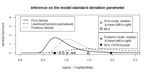
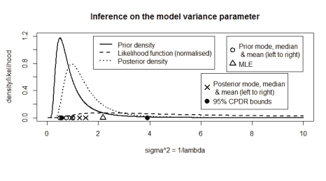
For the normal-gamma model defined by $\left(y_1, \ldots, y_n \mid \mu\right) \sim$ iid $N(\mu, 1 / \lambda)$ and $\lambda \sim \operatorname{Gamma}(\alpha, \beta)$, an uninformative prior is given by $\alpha=\beta=0$, that is, $f(\lambda) \propto 1 / \lambda, \lambda>0$.

For the binomial-beta model defined by $(y \mid \theta) \sim \operatorname{Binomial}(n, \theta)$ and $\theta \sim \operatorname{Beta}(\alpha, \beta)$ (having the posterior $(\theta \mid y) \sim \operatorname{Beta}(\alpha+y, \beta+n-y)$ ), an uninformative prior is the Bayes prior given by $\alpha=\beta=1$, that is, $f(\theta)=1,0<\theta<1$. This is the prior that was originally advocated by Thomas Bayes.

Unlike for the normal-normal and normal-gamma models, more than one uninformative prior specification has been proposed as reasonable in the context of the binomial-beta model.

One of these is the improper Haldane prior, defined by $\alpha=\beta=0$, or
$$
f(\theta) \propto \frac{1}{\theta(1-\theta)}, \quad 0<\theta<1 .
$$
Under the prior $\theta \sim \operatorname{Beta}(\alpha, \beta)$ generally, the posterior mean of $\theta$ is
$$
\hat{\theta}=E(\theta \mid y)=\frac{(\alpha+y)}{(\alpha+y)+(\beta+n-y)}=\frac{\alpha+y}{\alpha+\beta+n} .
$$
This reduces to the MLE $y / n$ under the Haldane prior but not under the Bayes prior. In contrast, the Bayes prior leads to a posterior mode which is equal to the MLE.

统计代写|贝叶斯分析代写Bayesian Analysis代考|The Jeffreys prior

The statistician Harold Jeffreys devised a rule for finding a suitable uninformative prior in a wide variety of situations. His idea was to construct a prior which is invariant under reparameterisation. For the case of a univariate model parameter $\theta$, the Jeffreys prior is given by the following equation (also known as Jeffreys’ rule):
$$
f(\theta) \propto \sqrt{I(\theta)}
$$
where $I(\theta)$ is the Fisher information defined by
$$
I(\theta)=E\left{\left(\frac{\partial}{\partial \theta} \log f(y \mid \theta)\right)^2 \mid \theta\right} .
$$
Note 1: If $\log f(y \mid \theta)$ is twice differentiable with respect to $\theta$, and certain regularity conditions hold, then
$$
I(\theta)=-E\left{\frac{\partial^2}{\partial \theta^2} \log f(y \mid \theta) \mid \theta\right} .
$$
Note 2: Jeffreys’ rule also extends to the multi-parameter case (not considered here).

The significance of Jeffreys’ rule may be described as follows. Consider a prior given by $f(\theta) \propto \sqrt{I(\theta)}$ and the transformed parameter $\phi=g(\theta)$,where $g$ is a strictly increasing or decreasing function. (For simplicity, we only consider this case.) Then the prior density for $\phi$ is
$f(\phi) \propto f(\theta)\left|\frac{\partial \theta}{\partial \phi}\right|$ by the transformation rule
$$
\begin{aligned}
& \propto \sqrt{I(\theta)\left(\frac{\partial \theta}{\partial \phi}\right)^2}=\sqrt{E\left{\left(\frac{\partial}{\partial \theta} \log f(y \mid \theta)\right)^2 \mid \theta\right}\left(\frac{\partial \theta}{\partial \phi}\right)^2} \
& =\sqrt{E\left{\left(\frac{\partial}{\partial \theta} \log f(y \mid \theta) \frac{\partial \theta}{\partial \phi}\right)^2 \mid \theta\right}} \
& =\sqrt{E\left{\left(\frac{\partial}{\partial \phi} \log f(y \mid \phi)\right)^2 \mid \phi\right}} \
& =\sqrt{I(\phi)} .
\end{aligned}
$$
Thus, Jeffreys’ rule is ‘invariant under reparameterisation’, in the sense that if a prior is constructed according to
$$
f(\theta) \propto \sqrt{I(\theta)}
$$
then, for another parameter $\phi=g(\theta)$, it is also true that
$$
f(\phi) \propto \sqrt{I(\phi)} .
$$

统计代写|贝叶斯分析代写Bayesian Analysis代考|Dealing with a priori ignorance

贝叶斯分析代考

统计代写|贝叶斯分析代写Bayesian Analysis代考|Dealing with a priori ignorance

即使存在完全(或完全)先验无知(意味着根本没有先验信息),贝叶斯方法也需要指定先验分布。这一特征提出了贝叶斯范式的一个普遍的哲学问题,其中有几个理论解决方案已经提出,但还没有一个普遍接受的解决方案。我们已经讨论了寻找与特定贝叶斯模型相关的无信息先验,如下所示。

对于$\left(y_1, \ldots, y_n \mid \mu\right) \sim$ iid $N\left(\mu, \sigma^2\right)$和$\mu \sim N\left(\mu_0, \sigma_0^2\right)$定义的正态-正态模型,无信息先验由$\sigma_0=\infty$给出,即$f(\mu) \propto 1, \mu \in \Re$。

对于由$\left(y_1, \ldots, y_n \mid \mu\right) \sim$ iid $N(\mu, 1 / \lambda)$和$\lambda \sim \operatorname{Gamma}(\alpha, \beta)$定义的正态伽玛模型,无信息先验由$\alpha=\beta=0$给出,即$f(\lambda) \propto 1 / \lambda, \lambda>0$。

对于由$(y \mid \theta) \sim \operatorname{Binomial}(n, \theta)$和$\theta \sim \operatorname{Beta}(\alpha, \beta)$(具有后验$(\theta \mid y) \sim \operatorname{Beta}(\alpha+y, \beta+n-y)$)定义的二项- β模型,无信息先验是$\alpha=\beta=1$给出的贝叶斯先验,即$f(\theta)=1,0<\theta<1$。这是Thomas Bayes最初提倡的先验。

与正态-正态和正态-伽马模型不同,在二项- β模型的背景下,不止一个无信息的先前规范被认为是合理的。

其中之一是不正确的霍尔丹先验,由$\alpha=\beta=0$或定义
$$
f(\theta) \propto \frac{1}{\theta(1-\theta)}, \quad 0<\theta<1 .
$$
在先验$\theta \sim \operatorname{Beta}(\alpha, \beta)$下,$\theta$的后验均值一般为
$$
\hat{\theta}=E(\theta \mid y)=\frac{(\alpha+y)}{(\alpha+y)+(\beta+n-y)}=\frac{\alpha+y}{\alpha+\beta+n} .
$$
这简化为在霍尔丹先验下的MLE $y / n$,而不是在贝叶斯先验下。相比之下,贝叶斯先验导致的后验模式等于最大似然。

统计代写|贝叶斯分析代写Bayesian Analysis代考|The Jeffreys prior

统计学家哈罗德·杰弗里斯(Harold Jeffreys)设计了一条规则,用于在各种各样的情况下找到合适的非信息先验。他的想法是构造一个在重参数化下不变的先验。对于单变量模型参数$\theta$,杰弗里斯先验由下式给出(也称为杰弗里斯规则):
$$
f(\theta) \propto \sqrt{I(\theta)}
$$
哪里$I(\theta)$是费雪信息的定义
$$
I(\theta)=E\left{\left(\frac{\partial}{\partial \theta} \log f(y \mid \theta)\right)^2 \mid \theta\right} .
$$
注1:如果$\log f(y \mid \theta)$对$\theta$是二次可微的,且一定的正则性条件成立,则
$$
I(\theta)=-E\left{\frac{\partial^2}{\partial \theta^2} \log f(y \mid \theta) \mid \theta\right} .
$$
注2:Jeffreys规则也适用于多参数情况(此处不考虑)。

杰弗里斯规则的意义可以描述如下。考虑$f(\theta) \propto \sqrt{I(\theta)}$给出的先验和转换后的参数$\phi=g(\theta)$,其中$g$是严格的递增或递减函数。(为简单起见,我们只考虑这种情况。)那么$\phi$的先验密度为
通过变换规则$f(\phi) \propto f(\theta)\left|\frac{\partial \theta}{\partial \phi}\right|$
$$
\begin{aligned}
& \propto \sqrt{I(\theta)\left(\frac{\partial \theta}{\partial \phi}\right)^2}=\sqrt{E\left{\left(\frac{\partial}{\partial \theta} \log f(y \mid \theta)\right)^2 \mid \theta\right}\left(\frac{\partial \theta}{\partial \phi}\right)^2} \
& =\sqrt{E\left{\left(\frac{\partial}{\partial \theta} \log f(y \mid \theta) \frac{\partial \theta}{\partial \phi}\right)^2 \mid \theta\right}} \
& =\sqrt{E\left{\left(\frac{\partial}{\partial \phi} \log f(y \mid \phi)\right)^2 \mid \phi\right}} \
& =\sqrt{I(\phi)} .
\end{aligned}
$$
因此,杰弗里斯的规则是“在重新参数化下不变的”,在这个意义上,如果一个先验是根据
$$
f(\theta) \propto \sqrt{I(\theta)}
$$
那么,对于另一个参数$\phi=g(\theta)$,也是成立的
$$
f(\phi) \propto \sqrt{I(\phi)} .
$$

统计代写|贝叶斯分析代写Bayesian Analysis代考 请认准statistics-lab™

统计代写请认准statistics-lab™. statistics-lab™为您的留学生涯保驾护航。

金融工程代写

金融工程是使用数学技术来解决金融问题。金融工程使用计算机科学、统计学、经济学和应用数学领域的工具和知识来解决当前的金融问题,以及设计新的和创新的金融产品。

非参数统计代写

非参数统计指的是一种统计方法,其中不假设数据来自于由少数参数决定的规定模型;这种模型的例子包括正态分布模型和线性回归模型。

广义线性模型代考

广义线性模型(GLM)归属统计学领域,是一种应用灵活的线性回归模型。该模型允许因变量的偏差分布有除了正态分布之外的其它分布。

术语 广义线性模型(GLM)通常是指给定连续和/或分类预测因素的连续响应变量的常规线性回归模型。它包括多元线性回归,以及方差分析和方差分析(仅含固定效应)。

有限元方法代写

有限元方法(FEM)是一种流行的方法,用于数值解决工程和数学建模中出现的微分方程。典型的问题领域包括结构分析、传热、流体流动、质量运输和电磁势等传统领域。

有限元是一种通用的数值方法,用于解决两个或三个空间变量的偏微分方程(即一些边界值问题)。为了解决一个问题,有限元将一个大系统细分为更小、更简单的部分,称为有限元。这是通过在空间维度上的特定空间离散化来实现的,它是通过构建对象的网格来实现的:用于求解的数值域,它有有限数量的点。边界值问题的有限元方法表述最终导致一个代数方程组。该方法在域上对未知函数进行逼近。[1] 然后将模拟这些有限元的简单方程组合成一个更大的方程系统,以模拟整个问题。然后,有限元通过变化微积分使相关的误差函数最小化来逼近一个解决方案。

tatistics-lab作为专业的留学生服务机构,多年来已为美国、英国、加拿大、澳洲等留学热门地的学生提供专业的学术服务,包括但不限于Essay代写,Assignment代写,Dissertation代写,Report代写,小组作业代写,Proposal代写,Paper代写,Presentation代写,计算机作业代写,论文修改和润色,网课代做,exam代考等等。写作范围涵盖高中,本科,研究生等海外留学全阶段,辐射金融,经济学,会计学,审计学,管理学等全球99%专业科目。写作团队既有专业英语母语作者,也有海外名校硕博留学生,每位写作老师都拥有过硬的语言能力,专业的学科背景和学术写作经验。我们承诺100%原创,100%专业,100%准时,100%满意。

随机分析代写


随机微积分是数学的一个分支,对随机过程进行操作。它允许为随机过程的积分定义一个关于随机过程的一致的积分理论。这个领域是由日本数学家伊藤清在第二次世界大战期间创建并开始的。

时间序列分析代写

随机过程,是依赖于参数的一组随机变量的全体,参数通常是时间。 随机变量是随机现象的数量表现,其时间序列是一组按照时间发生先后顺序进行排列的数据点序列。通常一组时间序列的时间间隔为一恒定值(如1秒,5分钟,12小时,7天,1年),因此时间序列可以作为离散时间数据进行分析处理。研究时间序列数据的意义在于现实中,往往需要研究某个事物其随时间发展变化的规律。这就需要通过研究该事物过去发展的历史记录,以得到其自身发展的规律。

回归分析代写

多元回归分析渐进(Multiple Regression Analysis Asymptotics)属于计量经济学领域,主要是一种数学上的统计分析方法,可以分析复杂情况下各影响因素的数学关系,在自然科学、社会和经济学等多个领域内应用广泛。

MATLAB代写

MATLAB 是一种用于技术计算的高性能语言。它将计算、可视化和编程集成在一个易于使用的环境中,其中问题和解决方案以熟悉的数学符号表示。典型用途包括:数学和计算算法开发建模、仿真和原型制作数据分析、探索和可视化科学和工程图形应用程序开发,包括图形用户界面构建MATLAB 是一个交互式系统,其基本数据元素是一个不需要维度的数组。这使您可以解决许多技术计算问题,尤其是那些具有矩阵和向量公式的问题,而只需用 C 或 Fortran 等标量非交互式语言编写程序所需的时间的一小部分。MATLAB 名称代表矩阵实验室。MATLAB 最初的编写目的是提供对由 LINPACK 和 EISPACK 项目开发的矩阵软件的轻松访问,这两个项目共同代表了矩阵计算软件的最新技术。MATLAB 经过多年的发展,得到了许多用户的投入。在大学环境中,它是数学、工程和科学入门和高级课程的标准教学工具。在工业领域,MATLAB 是高效研究、开发和分析的首选工具。MATLAB 具有一系列称为工具箱的特定于应用程序的解决方案。对于大多数 MATLAB 用户来说非常重要,工具箱允许您学习应用专业技术。工具箱是 MATLAB 函数(M 文件)的综合集合,可扩展 MATLAB 环境以解决特定类别的问题。可用工具箱的领域包括信号处理、控制系统、神经网络、模糊逻辑、小波、仿真等。

R语言代写问卷设计与分析代写
PYTHON代写回归分析与线性模型代写
MATLAB代写方差分析与试验设计代写
STATA代写机器学习/统计学习代写
SPSS代写计量经济学代写
EVIEWS代写时间序列分析代写
EXCEL代写深度学习代写
SQL代写各种数据建模与可视化代写

统计代写|贝叶斯分析代写Bayesian Analysis代考|Bayesian point estimation

如果你也在 怎样代写贝叶斯分析Bayesian Analysis 这个学科遇到相关的难题,请随时右上角联系我们的24/7代写客服。贝叶斯分析Bayesian Analysis一种统计推断方法(以英国数学家托马斯-贝叶斯命名),它允许人们将关于人口参数的先验信息与样本中包含的信息证据相结合,以指导统计推断过程。首先指定一个感兴趣的参数的先验概率分布。然后通过应用贝叶斯定理获得并结合证据,为参数提供一个后验概率分布。后验分布为有关该参数的统计推断提供了基础。

贝叶斯分析,一种统计推断方法(以英国数学家托马斯-贝叶斯命名),允许人们将关于人口参数的先验信息与样本所含信息的证据相结合,以指导统计推断过程。

statistics-lab™ 为您的留学生涯保驾护航 在代写贝叶斯分析Bayesian Analysis方面已经树立了自己的口碑, 保证靠谱, 高质且原创的统计Statistics代写服务。我们的专家在代写贝叶斯分析Bayesian Analysis代写方面经验极为丰富,各种代写贝叶斯分析Bayesian Analysis相关的作业也就用不着说。

统计代写|贝叶斯分析代写Bayesian Analysis代考|Bayesian point estimation

统计代写|贝叶斯分析代写Bayesian Analysis代考|Bayesian point estimation

Once the posterior distribution or density $f(\theta \mid y)$ has been obtained, Bayesian point estimates of the model parameter $\theta$ can be calculated. The three most commonly used point estimates are as follows.

The posterior mean of $\theta$ is
$$
E(\theta \mid y)=\int \theta d F(\theta \mid y)=\left{\begin{array}{cl}
\int \theta f(\theta \mid y) d \theta & \text { if } \theta \text { is continuous } \
\sum_\theta \theta f(\theta \mid y) & \text { if } \theta \text { is discrete. }
\end{array}\right.
$$

The posterior mode of $\theta$ is
$\operatorname{Mode}(\theta \mid y)=$ any value $m \in \Re$ which satisfies
$$
f(\theta=m \mid x)=\max \theta f(\theta \mid x) $$ or $\lim {\theta \rightarrow m} f(\theta \mid x)=\sup f(\theta \mid x)$,
or the set of all such values.

The posterior median of $\theta$ is
$\operatorname{Median}(\theta \mid y)=$ any value $m$ of $\theta$ such that
$$
\begin{aligned}
& P(\theta \leq m \mid y) \geq 1 / 2 \
& \text { and } P(\theta \geq m \mid y) \geq 1 / 2 \text {, } \
&
\end{aligned}
$$
or the set of all such values.

统计代写|贝叶斯分析代写Bayesian Analysis代考|Bayesian interval estimation

There are many ways to construct a Bayesian interval estimate, but the two most common ways are defined as follows. The $1-\alpha$ (or $100(1-\alpha) \%$ ) highest posterior density region (HPDR) for $\theta$ is the smallest set $S$ such that:
$$
P(\theta \in S \mid y) \geq 1-\alpha
$$
and $f\left(\theta_1 \mid y\right) \geq f\left(\theta_2 \mid y\right)$ if $\theta_1 \in S$ and $\theta_2 \notin S$.
Figure 1.6 illustrates the idea of the HPDR. In the very common situation where $\theta$ is scalar, continuous and has a posterior density which is unimodal with no local modes (i.e. has the form of a single ‘mound’), the $1-\alpha$ HPDR takes on the form of a single interval defined by two points at which the posterior density has the same value. When the HPDR is a single interval, it is the shortest possible single interval over which the area under the posterior density is $1-\alpha$.

The $1-\alpha$ central posterior density region (CPDR) for a scalar parameter $\theta$ may be defined as the shortest single interval $[a, b]$ such that:
$$
P(\thetab \mid y) \leq \alpha / 2$.

In the common case of a continuous parameter with a posterior density in the form of a single ‘mound’ which is furthermore symmetric, the CPDR and HPDR are identical.

统计代写|贝叶斯分析代写Bayesian Analysis代考|Bayesian point estimation

贝叶斯分析代考

统计代写|贝叶斯分析代写Bayesian Analysis代考|Bayesian point estimation

一旦获得后验分布或密度$f(\theta \mid y)$,就可以计算模型参数$\theta$的贝叶斯点估计。三种最常用的点估计如下。

$\ $的后验均值是
$ $
E(\theta \mid y)=\int \theta d F(\theta \mid y)=\left{\begin{array}{cl}
\int \theta f(\theta \mid y) d \theta & \text {if} \theta \text{是连续的}
\sum_\theta \theta f(\theta \mid y) & \text {if} \theta \text{是离散的。}
数组{}\ \端。
$ $

$\ $的后验模式是
$\operatorname{Mode}(\theta \mid y)=$任意值$m \in \Re$满足
$ $
F (\theta=m \mid x)=\max \theta F (\theta \mid x)$ $或$\lim {\theta \right row m} F (\theta \mid x)=\sup F (\theta \mid x)$ $,
或者说所有这些值的集合。

$\ $的后中位数是
$\operatorname{Median}(\theta \mid y)=$ \theta$的任意值$m$
$ $
开始{对齐}
& P(\theta \leq m \mid y) \geq 1 / 2 \
& \text {and} P(\theta \geq m \mid y) \geq 1 / 2 \text {,} \
&
结束{对齐}
$ $
或者说所有这些值的集合。

统计代写|贝叶斯分析代写Bayesian Analysis代考|Bayesian interval estimation

有许多方法可以构造贝叶斯区间估计,但最常见的两种方法定义如下。$\theta$的$1-\alpha$(或$100(1-\alpha) \%$)最高后验密度区域(HPDR)是满足以下条件的最小集合$S$:
$ $
P(\theta \in S \mid y) \geq 1-\ α
$ $
$f\left(\theta_1 \mid y\right)$ geq f\left(\theta_2 \mid y\right)$ if $\theta_1 \in S$和$\theta_2 \notin S$。
图1.6说明了HPDR的思想。在非常常见的情况下,$\theta$是标量的,连续的,并且具有单峰的无局部模态的后验密度(即具有单个“丘”的形式),$1-\alpha$ HPDR采用由两个后验密度具有相同值的点定义的单个区间的形式。当HPDR为单个区间时,它是后验密度下的面积为$1-\alpha$的最短可能的单个区间。

标量参数$\theta$的$1- $中央后验密度区域(CPDR)可以定义为满足以下条件的最短单区间$[a, b]$:
$ $
P(\thetab \mid y) \leq \alpha / 2$。

在一般情况下,一个连续参数的后验密度为一个进一步对称的“堆”形式,CPDR和HPDR是相同的。

统计代写|贝叶斯分析代写Bayesian Analysis代考 请认准statistics-lab™

统计代写请认准statistics-lab™. statistics-lab™为您的留学生涯保驾护航。

金融工程代写

金融工程是使用数学技术来解决金融问题。金融工程使用计算机科学、统计学、经济学和应用数学领域的工具和知识来解决当前的金融问题,以及设计新的和创新的金融产品。

非参数统计代写

非参数统计指的是一种统计方法,其中不假设数据来自于由少数参数决定的规定模型;这种模型的例子包括正态分布模型和线性回归模型。

广义线性模型代考

广义线性模型(GLM)归属统计学领域,是一种应用灵活的线性回归模型。该模型允许因变量的偏差分布有除了正态分布之外的其它分布。

术语 广义线性模型(GLM)通常是指给定连续和/或分类预测因素的连续响应变量的常规线性回归模型。它包括多元线性回归,以及方差分析和方差分析(仅含固定效应)。

有限元方法代写

有限元方法(FEM)是一种流行的方法,用于数值解决工程和数学建模中出现的微分方程。典型的问题领域包括结构分析、传热、流体流动、质量运输和电磁势等传统领域。

有限元是一种通用的数值方法,用于解决两个或三个空间变量的偏微分方程(即一些边界值问题)。为了解决一个问题,有限元将一个大系统细分为更小、更简单的部分,称为有限元。这是通过在空间维度上的特定空间离散化来实现的,它是通过构建对象的网格来实现的:用于求解的数值域,它有有限数量的点。边界值问题的有限元方法表述最终导致一个代数方程组。该方法在域上对未知函数进行逼近。[1] 然后将模拟这些有限元的简单方程组合成一个更大的方程系统,以模拟整个问题。然后,有限元通过变化微积分使相关的误差函数最小化来逼近一个解决方案。

tatistics-lab作为专业的留学生服务机构,多年来已为美国、英国、加拿大、澳洲等留学热门地的学生提供专业的学术服务,包括但不限于Essay代写,Assignment代写,Dissertation代写,Report代写,小组作业代写,Proposal代写,Paper代写,Presentation代写,计算机作业代写,论文修改和润色,网课代做,exam代考等等。写作范围涵盖高中,本科,研究生等海外留学全阶段,辐射金融,经济学,会计学,审计学,管理学等全球99%专业科目。写作团队既有专业英语母语作者,也有海外名校硕博留学生,每位写作老师都拥有过硬的语言能力,专业的学科背景和学术写作经验。我们承诺100%原创,100%专业,100%准时,100%满意。

随机分析代写


随机微积分是数学的一个分支,对随机过程进行操作。它允许为随机过程的积分定义一个关于随机过程的一致的积分理论。这个领域是由日本数学家伊藤清在第二次世界大战期间创建并开始的。

时间序列分析代写

随机过程,是依赖于参数的一组随机变量的全体,参数通常是时间。 随机变量是随机现象的数量表现,其时间序列是一组按照时间发生先后顺序进行排列的数据点序列。通常一组时间序列的时间间隔为一恒定值(如1秒,5分钟,12小时,7天,1年),因此时间序列可以作为离散时间数据进行分析处理。研究时间序列数据的意义在于现实中,往往需要研究某个事物其随时间发展变化的规律。这就需要通过研究该事物过去发展的历史记录,以得到其自身发展的规律。

回归分析代写

多元回归分析渐进(Multiple Regression Analysis Asymptotics)属于计量经济学领域,主要是一种数学上的统计分析方法,可以分析复杂情况下各影响因素的数学关系,在自然科学、社会和经济学等多个领域内应用广泛。

MATLAB代写

MATLAB 是一种用于技术计算的高性能语言。它将计算、可视化和编程集成在一个易于使用的环境中,其中问题和解决方案以熟悉的数学符号表示。典型用途包括:数学和计算算法开发建模、仿真和原型制作数据分析、探索和可视化科学和工程图形应用程序开发,包括图形用户界面构建MATLAB 是一个交互式系统,其基本数据元素是一个不需要维度的数组。这使您可以解决许多技术计算问题,尤其是那些具有矩阵和向量公式的问题,而只需用 C 或 Fortran 等标量非交互式语言编写程序所需的时间的一小部分。MATLAB 名称代表矩阵实验室。MATLAB 最初的编写目的是提供对由 LINPACK 和 EISPACK 项目开发的矩阵软件的轻松访问,这两个项目共同代表了矩阵计算软件的最新技术。MATLAB 经过多年的发展,得到了许多用户的投入。在大学环境中,它是数学、工程和科学入门和高级课程的标准教学工具。在工业领域,MATLAB 是高效研究、开发和分析的首选工具。MATLAB 具有一系列称为工具箱的特定于应用程序的解决方案。对于大多数 MATLAB 用户来说非常重要,工具箱允许您学习应用专业技术。工具箱是 MATLAB 函数(M 文件)的综合集合,可扩展 MATLAB 环境以解决特定类别的问题。可用工具箱的领域包括信号处理、控制系统、神经网络、模糊逻辑、小波、仿真等。

R语言代写问卷设计与分析代写
PYTHON代写回归分析与线性模型代写
MATLAB代写方差分析与试验设计代写
STATA代写机器学习/统计学习代写
SPSS代写计量经济学代写
EVIEWS代写时间序列分析代写
EXCEL代写深度学习代写
SQL代写各种数据建模与可视化代写

统计代写|贝叶斯分析代写Bayesian Analysis代考|The Evidence Idiom

如果你也在 怎样代写贝叶斯分析Bayesian Analysis这个学科遇到相关的难题,请随时右上角联系我们的24/7代写客服。

贝叶斯分析,一种统计推断方法(以英国数学家托马斯-贝叶斯命名),允许人们将关于人口参数的先验信息与样本所含信息的证据相结合,以指导统计推断过程。

statistics-lab™ 为您的留学生涯保驾护航 在代写贝叶斯分析Bayesian Analysis方面已经树立了自己的口碑, 保证靠谱, 高质且原创的统计Statistics代写服务。我们的专家在代写贝叶斯分析Bayesian Analysis代写方面经验极为丰富,各种代写贝叶斯分析Bayesian Analysis相关的作业也就用不着说。

我们提供的贝叶斯分析Bayesian Analysis及其相关学科的代写,服务范围广, 其中包括但不限于:

  • Statistical Inference 统计推断
  • Statistical Computing 统计计算
  • Advanced Probability Theory 高等概率论
  • Advanced Mathematical Statistics 高等数理统计学
  • (Generalized) Linear Models 广义线性模型
  • Statistical Machine Learning 统计机器学习
  • Longitudinal Data Analysis 纵向数据分析
  • Foundations of Data Science 数据科学基础

统计代写|贝叶斯分析代写Bayesian Analysis代考|The Evidence Idiom

We can think of the simple two-node BN (consisting of a hypothesis node $H$, i.e., a parent of an evidence node $E$ ) -and its extension to multiple pieces of evidence-as the most basic $\mathrm{BN}$ idiom for legal reasoning. This basic idiom, which we call the evidence idiom, is an instantiation of the cause-consequence idiom and has the generic structure shown in Figure 16.1.

We do not distinguish between evidence that supports the prosecution $(H$ true) and evidence that supports the defense $(H$ false), since the BN model handles both types of evidence seamlessly. Hence, this idiom subsumes two basic patterns:

  1. Corroboration pattern: this is simply the case where there are two pieces of evidence, E1 and E2, that both support one side of the argument.
  2. Conflict pattern: this is simply the case where there are two pieces of evidence, E1 and E2, with one supporting the prosecution and the other supporting the defense.
    The evidence idiom assumes that the various pieces of evidence are independent, and it is this assumption that makes it possible to compute the overall likelihood ratio for the combined evidence by simply multiplying the individual LRs (as we explained in Chapter 15). In other words, we do not need BN computations to calculate the LR. It is not surprising, therefore, that in practice, forensic experts try to force their evidence to fit this idiom. However, as we also discussed in Chapter 15 , in real cases, the assumption is oversimplistic, meaning that the evidence idiom has a number of limitations. The following idioms identify and address these various limitations in turn.

统计代写|贝叶斯分析代写Bayesian Analysis代考|The Evidence Accuracy Idiom

The evidence accuracy idiom (Figure 16.2) is the legal equivalent of the measurement idiom. Just as the measurement idiom is crucial for distinguishing between a potentially inaccurate “measured value” of some attribute and the true but unknown value itself (such as an IQ test to measure the intelligence of a person or a mobile phone app to measure the temperature outside), any piece of evidence in a legal case can be considered a potentially inaccurate assertion about the true value of some unknown hypothesis. So, when an expert witness testifies that a defendant had an excess amount of alcohol in his or her blood, we cannot treat this as being exactly the same as the fact that the defendant had an excess amount of alcohol in his or her blood. The expert could be using inaccurate test equipment or might make errors in reporting.

For simplicity, we have lumped together all possible sources of inaccuracy into a single node (see sidebar “Modeling Different Notions of ‘Accuracy”‘).

In general, what is often assumed to be a “single piece of evidence for a single hypothesis” turns out to be more realistically modeled by multiple instances of the evidence accuracy idiom.

In Chapter 15 , we explained the importance of including all relevant context when building a $\mathrm{BN}$ model to evaluate the probative value of legal evidence. In particular, our ultimate goal is to determine the impact of the evidence on the ultimate hypothesis (defendant is guilty). Hence, if we wish to build BNs for complete legal cases, we need to include the ultimate hypothesis as a node in the model. It may seem “correct” that such a node should have no parents, as this fits naturally with the intuitive approach to legal reasoning whereby it is the hypothesis about which we start with an unconditional prior belief before observing evidence to update that belief. However, there are two very common types of evidence that, unlike the examples seen so far, support hypotheses that are causes, rather than consequences, of guilt. These hypotheses are concerned with “opportunity” and “motive,” and they inevitably change the fundamental structure of the underlying causal model.

贝叶斯分析代考

统计代写|贝叶斯分析代写Bayesian Analysis代考|The Evidence Idiom

我们可以想到简单的双节点 BN(由一个假设节点组成H,即证据节点的父节点和)——及其对多条证据的扩展——作为最基本的乙否法律推理的成语。这个基本习语,我们称之为证据习语,是因果习语的一个实例,具有图 16.1 所示的通用结构。

我们不区分支持起诉的证据(H真)和支持辩护的证据(Hfalse),因为 BN 模型可以无缝处理这两种类型的证据。因此,这个成语包含两个基本模式:

  1. 确证模式:这是简单的情况,有两个证据,E1 和 E2,都支持论点的一方。
  2. 冲突模式:简单来说就是有两份证据E1和E2,一份支持控方,另一份支持辩方。
    证据习语假设各种证据是独立的,正是这种假设使得通过简单地乘以各个 LR 来计算组合证据的总体似然比成为可能(如我们在第 15 章中解释的那样)。换句话说,我们不需要 BN 计算来计算 LR。因此,在实践中,法医专家试图强制他们的证据符合这个习语也就不足为奇了。然而,正如我们在第 15 章中也讨论过的那样,在实际案例中,假设过于简单化,这意味着证据习语有许多局限性。以下成语依次识别和解决这些不同的限制。

统计代写|贝叶斯分析代写Bayesian Analysis代考|The Evidence Accuracy Idiom

证据准确性习语(图 16.2)是测量习语的法律等价物。正如测量习语对于区分某些属性的潜在不准确“测量值”和真实但未知的值本身(例如用于测量人智力的智商测试或用于测量室外温度的手机应用程序)至关重要), 法律案件中的任何证据都可以被认为是对某些未知假设的真实价值的潜在不准确断言。所以,当专家证人证明被告人血液中酒精含量超标时,我们不能把这与被告人血液中酒精含量超标的事实完全等同。专家可能使用了不准确的测试设备或可能在报告中出错。

为简单起见,我们将所有可能的不准确性来源集中到一个节点中(请参阅边栏“对“准确性”的不同概念进行建模”)。

总的来说,通常被认为是“单一假设的单一证据”的事实证明,证据准确性习语的多个实例更符合实际。

在第 15 章中,我们解释了在构建乙否评估法律证据证明力的模型。特别是,我们的最终目标是确定证据对最终假设(被告有罪)的影响。因此,如果我们希望为完整的法律案件构建 BN,我们需要将最终假设作为节点包含在模型中。这样的节点应该没有父节点似乎是“正确的”,因为这自然符合法律推理的直觉方法,即我们在观察证据以更新该信念之前从无条件先验信念开始的假设。然而,有两种非常常见的证据类型,与目前看到的例子不同,它们支持的假设是内疚的原因,而不是结果。这些假设与“机会”和“动机”有关,

统计代写|贝叶斯分析代写Bayesian Analysis代考 请认准statistics-lab™

统计代写请认准statistics-lab™. statistics-lab™为您的留学生涯保驾护航。

金融工程代写

金融工程是使用数学技术来解决金融问题。金融工程使用计算机科学、统计学、经济学和应用数学领域的工具和知识来解决当前的金融问题,以及设计新的和创新的金融产品。

非参数统计代写

非参数统计指的是一种统计方法,其中不假设数据来自于由少数参数决定的规定模型;这种模型的例子包括正态分布模型和线性回归模型。

广义线性模型代考

广义线性模型(GLM)归属统计学领域,是一种应用灵活的线性回归模型。该模型允许因变量的偏差分布有除了正态分布之外的其它分布。

术语 广义线性模型(GLM)通常是指给定连续和/或分类预测因素的连续响应变量的常规线性回归模型。它包括多元线性回归,以及方差分析和方差分析(仅含固定效应)。

有限元方法代写

有限元方法(FEM)是一种流行的方法,用于数值解决工程和数学建模中出现的微分方程。典型的问题领域包括结构分析、传热、流体流动、质量运输和电磁势等传统领域。

有限元是一种通用的数值方法,用于解决两个或三个空间变量的偏微分方程(即一些边界值问题)。为了解决一个问题,有限元将一个大系统细分为更小、更简单的部分,称为有限元。这是通过在空间维度上的特定空间离散化来实现的,它是通过构建对象的网格来实现的:用于求解的数值域,它有有限数量的点。边界值问题的有限元方法表述最终导致一个代数方程组。该方法在域上对未知函数进行逼近。[1] 然后将模拟这些有限元的简单方程组合成一个更大的方程系统,以模拟整个问题。然后,有限元通过变化微积分使相关的误差函数最小化来逼近一个解决方案。

tatistics-lab作为专业的留学生服务机构,多年来已为美国、英国、加拿大、澳洲等留学热门地的学生提供专业的学术服务,包括但不限于Essay代写,Assignment代写,Dissertation代写,Report代写,小组作业代写,Proposal代写,Paper代写,Presentation代写,计算机作业代写,论文修改和润色,网课代做,exam代考等等。写作范围涵盖高中,本科,研究生等海外留学全阶段,辐射金融,经济学,会计学,审计学,管理学等全球99%专业科目。写作团队既有专业英语母语作者,也有海外名校硕博留学生,每位写作老师都拥有过硬的语言能力,专业的学科背景和学术写作经验。我们承诺100%原创,100%专业,100%准时,100%满意。

随机分析代写


随机微积分是数学的一个分支,对随机过程进行操作。它允许为随机过程的积分定义一个关于随机过程的一致的积分理论。这个领域是由日本数学家伊藤清在第二次世界大战期间创建并开始的。

时间序列分析代写

随机过程,是依赖于参数的一组随机变量的全体,参数通常是时间。 随机变量是随机现象的数量表现,其时间序列是一组按照时间发生先后顺序进行排列的数据点序列。通常一组时间序列的时间间隔为一恒定值(如1秒,5分钟,12小时,7天,1年),因此时间序列可以作为离散时间数据进行分析处理。研究时间序列数据的意义在于现实中,往往需要研究某个事物其随时间发展变化的规律。这就需要通过研究该事物过去发展的历史记录,以得到其自身发展的规律。

回归分析代写

多元回归分析渐进(Multiple Regression Analysis Asymptotics)属于计量经济学领域,主要是一种数学上的统计分析方法,可以分析复杂情况下各影响因素的数学关系,在自然科学、社会和经济学等多个领域内应用广泛。

MATLAB代写

MATLAB 是一种用于技术计算的高性能语言。它将计算、可视化和编程集成在一个易于使用的环境中,其中问题和解决方案以熟悉的数学符号表示。典型用途包括:数学和计算算法开发建模、仿真和原型制作数据分析、探索和可视化科学和工程图形应用程序开发,包括图形用户界面构建MATLAB 是一个交互式系统,其基本数据元素是一个不需要维度的数组。这使您可以解决许多技术计算问题,尤其是那些具有矩阵和向量公式的问题,而只需用 C 或 Fortran 等标量非交互式语言编写程序所需的时间的一小部分。MATLAB 名称代表矩阵实验室。MATLAB 最初的编写目的是提供对由 LINPACK 和 EISPACK 项目开发的矩阵软件的轻松访问,这两个项目共同代表了矩阵计算软件的最新技术。MATLAB 经过多年的发展,得到了许多用户的投入。在大学环境中,它是数学、工程和科学入门和高级课程的标准教学工具。在工业领域,MATLAB 是高效研究、开发和分析的首选工具。MATLAB 具有一系列称为工具箱的特定于应用程序的解决方案。对于大多数 MATLAB 用户来说非常重要,工具箱允许您学习应用专业技术。工具箱是 MATLAB 函数(M 文件)的综合集合,可扩展 MATLAB 环境以解决特定类别的问题。可用工具箱的领域包括信号处理、控制系统、神经网络、模糊逻辑、小波、仿真等。

R语言代写问卷设计与分析代写
PYTHON代写回归分析与线性模型代写
MATLAB代写方差分析与试验设计代写
STATA代写机器学习/统计学习代写
SPSS代写计量经济学代写
EVIEWS代写时间序列分析代写
EXCEL代写深度学习代写
SQL代写各种数据建模与可视化代写

统计代写|贝叶斯分析代写Bayesian Analysis代考|Basics of Bayes for Reasoning about Legal Evidence

如果你也在 怎样代写贝叶斯分析Bayesian Analysis这个学科遇到相关的难题,请随时右上角联系我们的24/7代写客服。

贝叶斯分析,一种统计推断方法(以英国数学家托马斯-贝叶斯命名),允许人们将关于人口参数的先验信息与样本所含信息的证据相结合,以指导统计推断过程。

statistics-lab™ 为您的留学生涯保驾护航 在代写贝叶斯分析Bayesian Analysis方面已经树立了自己的口碑, 保证靠谱, 高质且原创的统计Statistics代写服务。我们的专家在代写贝叶斯分析Bayesian Analysis代写方面经验极为丰富,各种代写贝叶斯分析Bayesian Analysis相关的作业也就用不着说。

我们提供的贝叶斯分析Bayesian Analysis及其相关学科的代写,服务范围广, 其中包括但不限于:

  • Statistical Inference 统计推断
  • Statistical Computing 统计计算
  • Advanced Probability Theory 高等概率论
  • Advanced Mathematical Statistics 高等数理统计学
  • (Generalized) Linear Models 广义线性模型
  • Statistical Machine Learning 统计机器学习
  • Longitudinal Data Analysis 纵向数据分析
  • Foundations of Data Science 数据科学基础

统计代写|贝叶斯分析代写Bayesian Analysis代考|Basics of Bayes for Reasoning about Legal Evidence

Probabilistic reasoning of legal evidence often boils down to the simple BN model shown in Figure 15.1. The hypothesis $H$ is a statement whose truth value we seek to determine, but is generally unknown-and which may never be known with certainty.
Examples include:
“Defendant is guilty of the crime as charged” (this is an example of what is called an offense-level hypothesis, but also called the ultimate hypothesis, since in many criminal cases, it is ultimately the only hypothesis we are really interested in)

  • “Defendant was at the crime scene” (this is an example of what is often referred to as an activity-level hypothesis)
  • “Defendant was the source of DNA found at the crime scene” (this is an example of what is often referred to as a source-level hypothesis)

The evidence $E$ is a statement that claims to support either the hypothesis $H$ or the alternative hypothesis (which is the negation of $H$ ). For example, a statement by an eyewitness who claims he or she saw the defendant at the scene of the crime might be considered evidence to support any of the above types of hypotheses. Of special interest is forensic evidence, such as the example shown in the explicit BN of Figure 15.2. In this example, we assume:

  • The evidence $E$ is a DNA trace found at the scene of the crime (for simplicity, we assume the crime was committed on an island with 10,000 people who therefore represent the entire set of possible suspects).
  • The defendant was arrested and some of his DNA was sampled and analyzed (see Box 15.7 for the necessary background about DNA profiles).

统计代写|贝叶斯分析代写Bayesian Analysis代考|The Problems with Trying to Avoid Using Prior Probabilities with the Likelihood Ratio

It is possible to avoid the delicate and controversial issue of assigning a subjective prior probability to the ultimate hypothesis (or, indeed, to any specific hypothesis) if we instead are prepared to focus only on the “probabilistic value” of the evidence. Recall from Chapter 6 and the sidebar that the impact of any single piece of evidence $E$ on a hypothesis $H$ can be determined by considering only the likelihood ratio of $E$, which is the probability of seeing that evidence if $H$ is true (e.g., “defendant is guilty”) divided by the probability of seeing that evidence if $H$ is not true (e.g., “defendant is not guilty”), that is, $P(E \mid H)$ divided by $P(E \mid \operatorname{not} H)$.

In the DNA example of Figure 15.2, the likelihood ratio is 1000 (since the prosecution likelihood is 1 and the defense likelihood is $1 / 1000$ ). So this particular evidence is clearly very probative in favor of the prosecution hypothesis (that the suspect is the source of the DNA found at the crime scene). In court, the DNA expert would be able to present this likelihood ratio without making any assertions about the prior probability of the prosecution hypothesis by simply saying:
We are 1000 more times likely to find this evidence under the assumption that the prosecution hypothesis is true than under the assumption that the defense hypothesis is true.
While this is helpful, the extent to which it can lead a judge or jury to “believe” the prosecution hypothesis still depends on the prior probability; as explained in Box 15.9, we use the “odds” version of Bayes (that we introduced in Chapter 6) to make the necessary conclusions.

In summary, whether the likelihood ratio of 1000 -or even 10 million-“swings” the odds sufficiently in favor of the prosecution hypothesis depends entirely on the prior odds. So, while the likelihood ratio enables us to assess the impact of evidence on $H$ without having to consider the prior probability of $H$, it is clear from the above DNA example that the prior probability must ultimately be considered before returning a verdict. With or without a Bayesian approach, jurors and judges intuitively make assumptions about the prior probability and adjust this in light of the evidence. A key benefit of the Bayesian approach is to make explicit the ramifications of different prior assumptions. So, a judge could state something like the following where, say, the evidence has a likelihood ratio of one million:
Whatever you believed before about the possible guilt of the defendant, the evidence is one million times more likely if the defendant is guilty than if he is innocent. So, if you believed at the beginning that there was a 50:50 chance that the defendant was innocent, then it is only rational for you to conclude with the evidence that there is only a million to one chance the defendant really is innocent. On this basis you should return a guilty verdict. But if you believed at the beginning that the defendant is no more likely to be guilty than a million other people in the area, then it is only rational for you to conclude with the evidence that there is a $50: 50$ chance the defendant really is innocent. On that basis you should return a not guilty verdict.

贝叶斯分析代考

统计代写|贝叶斯分析代写Bayesian Analysis代考|Basics of Bayes for Reasoning about Legal Evidence

法律证据的概率推理通常归结为图 15.1 所示的简单 BN 模型。假设H是一个陈述,我们试图确定其真值,但通常是未知的——而且可能永远无法确定。
示例包括:
“被告犯有被指控的罪行”(这是所谓的犯罪级别假设的示例,但也称为最终假设,因为在许多刑事案件中,它最终是我们真正的唯一假设有兴趣)

  • “被告在犯罪现场”(这是通常被称为活动水平假设的一个例子)
  • “被告是在犯罪现场发现的 DNA 的来源”(这是通常被称为源级假设的一个例子)

证据和是声称支持假设的陈述H或替代假设(这是否定的H). 例如,目击者声称他或她在犯罪现场看到被告的陈述可能被视为支持上述任何类型假设的证据。特别感兴趣的是取证证据,例如图 15.2 的显式 BN 中显示的示例。在这个例子中,我们假设:

  • 证据和是在犯罪现场发现的 DNA 痕迹(为简单起见,我们假设犯罪发生在一个有 10,000 人的岛上,因此代表了所有可能的嫌疑人)。
  • 被告被捕,对他的一些 DNA 进行了取样和分析(有关 DNA 图谱的必要背景,请参见专栏 15.7)。

统计代写|贝叶斯分析代写Bayesian Analysis代考|The Problems with Trying to Avoid Using Prior Probabilities with the Likelihood Ratio

如果我们只关注证据的“概率值”,就可以避免将主观先验概率分配给最终假设(或者实际上,分配给任何特定假设)这一微妙而有争议的问题。回想一下第 6 章和侧边栏,任何单个证据的影响和假设H可以通过仅考虑似然比来确定和,这是看到该证据的概率,如果H是真的(例如,“被告有罪”)除以看到该证据的概率,如果H是不正确的(例如,“被告无罪”),也就是说,P(和∣H)除以P(和∣不是⁡H).

在图 15.2 的 DNA 示例中,似然比为 1000(因为起诉可能性为 1,而辩护可能性为1/1000). 因此,这一特定证据显然非常有利于起诉假设(嫌疑人是在犯罪现场发现的 DNA 的来源)。在法庭上,DNA 专家将能够在不对起诉假设的先验概率做出任何断言的情况下提出这种似然比,只需简单地说:在假设
起诉假设为真的情况下,我们找到该证据的可能性是 1000 倍在防御假说成立的假设下。
虽然这很有帮助,但它能在多大程度上让法官或陪审团“相信”起诉假设仍然取决于先验概率;正如专栏 15.9 中所解释的,我们使用贝叶斯的“几率”版本(我们在第 6 章中介绍过)来得出必要的结论。

总而言之,1000 甚至 1000 万的似然比是否“摇摆”概率足以支持起诉假设完全取决于先验概率。因此,虽然似然比使我们能够评估证据对H无需考虑先验概率H,从上面的DNA例子中可以看出,在返回判决之前最终必须考虑先验概率。无论是否使用贝叶斯方法,陪审员和法官都会凭直觉对先验概率做出假设,并根据证据对其进行调整。贝叶斯方法的一个主要好处是明确不同先验假设的后果。因此,法官可以陈述如下内容,例如,证据的似然比为一百万:
无论您之前对被告可能有罪的看法如何,如果被告有罪,证据的可能性是他无罪的一百万倍。因此,如果您一开始就认为被告有 50:50 的可能性是无辜的,那么您只能合理地得出结论,证据表明被告真正无罪的可能性只有百万分之一。在此基础上,您应该作出有罪判决。但是,如果您一开始就认为被告人有罪的可能性并不比该地区的其他 100 万人高,那么您就只能理性地得出结论,证据表明存在50:50被告真的是无辜的。在此基础上,您应该作出无罪判决。

统计代写|贝叶斯分析代写Bayesian Analysis代考 请认准statistics-lab™

统计代写请认准statistics-lab™. statistics-lab™为您的留学生涯保驾护航。

金融工程代写

金融工程是使用数学技术来解决金融问题。金融工程使用计算机科学、统计学、经济学和应用数学领域的工具和知识来解决当前的金融问题,以及设计新的和创新的金融产品。

非参数统计代写

非参数统计指的是一种统计方法,其中不假设数据来自于由少数参数决定的规定模型;这种模型的例子包括正态分布模型和线性回归模型。

广义线性模型代考

广义线性模型(GLM)归属统计学领域,是一种应用灵活的线性回归模型。该模型允许因变量的偏差分布有除了正态分布之外的其它分布。

术语 广义线性模型(GLM)通常是指给定连续和/或分类预测因素的连续响应变量的常规线性回归模型。它包括多元线性回归,以及方差分析和方差分析(仅含固定效应)。

有限元方法代写

有限元方法(FEM)是一种流行的方法,用于数值解决工程和数学建模中出现的微分方程。典型的问题领域包括结构分析、传热、流体流动、质量运输和电磁势等传统领域。

有限元是一种通用的数值方法,用于解决两个或三个空间变量的偏微分方程(即一些边界值问题)。为了解决一个问题,有限元将一个大系统细分为更小、更简单的部分,称为有限元。这是通过在空间维度上的特定空间离散化来实现的,它是通过构建对象的网格来实现的:用于求解的数值域,它有有限数量的点。边界值问题的有限元方法表述最终导致一个代数方程组。该方法在域上对未知函数进行逼近。[1] 然后将模拟这些有限元的简单方程组合成一个更大的方程系统,以模拟整个问题。然后,有限元通过变化微积分使相关的误差函数最小化来逼近一个解决方案。

tatistics-lab作为专业的留学生服务机构,多年来已为美国、英国、加拿大、澳洲等留学热门地的学生提供专业的学术服务,包括但不限于Essay代写,Assignment代写,Dissertation代写,Report代写,小组作业代写,Proposal代写,Paper代写,Presentation代写,计算机作业代写,论文修改和润色,网课代做,exam代考等等。写作范围涵盖高中,本科,研究生等海外留学全阶段,辐射金融,经济学,会计学,审计学,管理学等全球99%专业科目。写作团队既有专业英语母语作者,也有海外名校硕博留学生,每位写作老师都拥有过硬的语言能力,专业的学科背景和学术写作经验。我们承诺100%原创,100%专业,100%准时,100%满意。

随机分析代写


随机微积分是数学的一个分支,对随机过程进行操作。它允许为随机过程的积分定义一个关于随机过程的一致的积分理论。这个领域是由日本数学家伊藤清在第二次世界大战期间创建并开始的。

时间序列分析代写

随机过程,是依赖于参数的一组随机变量的全体,参数通常是时间。 随机变量是随机现象的数量表现,其时间序列是一组按照时间发生先后顺序进行排列的数据点序列。通常一组时间序列的时间间隔为一恒定值(如1秒,5分钟,12小时,7天,1年),因此时间序列可以作为离散时间数据进行分析处理。研究时间序列数据的意义在于现实中,往往需要研究某个事物其随时间发展变化的规律。这就需要通过研究该事物过去发展的历史记录,以得到其自身发展的规律。

回归分析代写

多元回归分析渐进(Multiple Regression Analysis Asymptotics)属于计量经济学领域,主要是一种数学上的统计分析方法,可以分析复杂情况下各影响因素的数学关系,在自然科学、社会和经济学等多个领域内应用广泛。

MATLAB代写

MATLAB 是一种用于技术计算的高性能语言。它将计算、可视化和编程集成在一个易于使用的环境中,其中问题和解决方案以熟悉的数学符号表示。典型用途包括:数学和计算算法开发建模、仿真和原型制作数据分析、探索和可视化科学和工程图形应用程序开发,包括图形用户界面构建MATLAB 是一个交互式系统,其基本数据元素是一个不需要维度的数组。这使您可以解决许多技术计算问题,尤其是那些具有矩阵和向量公式的问题,而只需用 C 或 Fortran 等标量非交互式语言编写程序所需的时间的一小部分。MATLAB 名称代表矩阵实验室。MATLAB 最初的编写目的是提供对由 LINPACK 和 EISPACK 项目开发的矩阵软件的轻松访问,这两个项目共同代表了矩阵计算软件的最新技术。MATLAB 经过多年的发展,得到了许多用户的投入。在大学环境中,它是数学、工程和科学入门和高级课程的标准教学工具。在工业领域,MATLAB 是高效研究、开发和分析的首选工具。MATLAB 具有一系列称为工具箱的特定于应用程序的解决方案。对于大多数 MATLAB 用户来说非常重要,工具箱允许您学习应用专业技术。工具箱是 MATLAB 函数(M 文件)的综合集合,可扩展 MATLAB 环境以解决特定类别的问题。可用工具箱的领域包括信号处理、控制系统、神经网络、模糊逻辑、小波、仿真等。

R语言代写问卷设计与分析代写
PYTHON代写回归分析与线性模型代写
MATLAB代写方差分析与试验设计代写
STATA代写机器学习/统计学习代写
SPSS代写计量经济学代写
EVIEWS代写时间序列分析代写
EXCEL代写深度学习代写
SQL代写各种数据建模与可视化代写

统计代写|贝叶斯分析代写Bayesian Analysis代考|Context and Review of Bayes in Legal Proceedings

如果你也在 怎样代写贝叶斯分析Bayesian Analysis这个学科遇到相关的难题,请随时右上角联系我们的24/7代写客服。

贝叶斯分析,一种统计推断方法(以英国数学家托马斯-贝叶斯命名),允许人们将关于人口参数的先验信息与样本所含信息的证据相结合,以指导统计推断过程。

statistics-lab™ 为您的留学生涯保驾护航 在代写贝叶斯分析Bayesian Analysis方面已经树立了自己的口碑, 保证靠谱, 高质且原创的统计Statistics代写服务。我们的专家在代写贝叶斯分析Bayesian Analysis代写方面经验极为丰富,各种代写贝叶斯分析Bayesian Analysis相关的作业也就用不着说。

我们提供的贝叶斯分析Bayesian Analysis及其相关学科的代写,服务范围广, 其中包括但不限于:

  • Statistical Inference 统计推断
  • Statistical Computing 统计计算
  • Advanced Probability Theory 高等概率论
  • Advanced Mathematical Statistics 高等数理统计学
  • (Generalized) Linear Models 广义线性模型
  • Statistical Machine Learning 统计机器学习
  • Longitudinal Data Analysis 纵向数据分析
  • Foundations of Data Science 数据科学基础

统计代写|贝叶斯分析代写Bayesian Analysis代考|Context and Review of Bayes in Legal Proceedings

The use of statistics in legal proceedings (both criminal and civil) has a long, but not terribly distinguished, history. This is well documented in the references at the end of this chapter. The earliest reported case of a detailed statistical analysis being presented as evidence was in the Howland case in 1867. In this case, Benjamin Peirce attempted to show that a contested signature on a will had been traced from the genuine signature by arguing that their agreement in all 30 downstrokes was extremely improbable under a binomial model. However, there were misuses of the “product rule” in Peirce’s evidence for multiplying probabilities of independent events. In any case, the court found a technical excuse not to use the evidence.

The historical reticence to accept statistical analysis as valid evidence is, sadly, not without good reason. When, in 1894, a statistical analysis was used in the Dreyfus case, it turned out to be fundamentally flawed. Not until 1968 was there another well-documented case in which statistical analysis played a key role. In that case, another flawed statistical argument further set back the cause of statistics in court. The Collins case (see Box 15.1) was characterized by two errors:

  1. It underestimated the probability that some evidence would be observed if the defendants were innocent by failing to consider dependence between components of the evidence.
  2. It implied that the low probability from the calculation in (1) was synonymous with innocence (the so-called “prosecutor’s fallacy” that we introduced in Chapter 6 and will discuss further in Section 15.3).

Since then, the same errors (either in combination or individually) have occurred in other cases. One of the most notorious was that of $R$ v Sally Clark (Box 15.2).

The Lucia de Berk case (see Box 15.3) is another example whereby a prosecution case was fitted around the fact that one person was connected to a number of related deaths. People die in hospitals, and it is inevitable that there will be instances of individual nurses associated with much higher than normal death rates in any given period of time. The extremely low probability P(evidence I not guilty) – which, without any real evidence that the defendant has committed a crime, tells us very little-was used to drive the prosecution case. Another very similar case (currently subject to an appeal based on precisely these concerns) is that of Ben Geen, who was also a nurse convicted of multiple murders and attempted murder.

统计代写|贝叶斯分析代写Bayesian Analysis代考|Basics of Bayes for Reasoning about Legal Evidence

Probabilistic reasoning of legal evidence often boils down to the simple BN model shown in Figure 15.1. The hypothesis $H$ is a statement whose truth value we seek to determine, but is generally unknown-and which may never be known with certainty.
Examples include:

  • “Defendant is guilty of the crime as charged” (this is an example of what is called an offense-level hypothesis, but also called the ultimate hypothesis, since in many criminal cases, it is ultimately the only hypothesis we are really interested in)
  • “Defendant was at the crime scene” (this is an example of what is often referred to as an activity-level hypothesis)
  • “Defendant was the source of DNA found at the crime scene” (this is an example of what is often referred to as a source-level hypothesis)

The evidence $E$ is a statement that claims to support either the hypothesis $H$ or the alternative hypothesis (which is the negation of $H$ ). For example, a statement by an eyewitness who claims he or she saw the defendant at the scene of the crime might be considered evidence to support any of the above types of hypotheses. Of special interest is forensic evidence, such as the example shown in the explicit BN of Figure 15.2. In this example, we assume:

  • The evidence $E$ is a DNA trace found at the scene of the crime (for simplicity, we assume the crime was committed on an island with 10,000 people who therefore represent the entire set of possible suspects).
  • The defendant was arrested and some of his DNA was sampled and analyzed (see Box 15.7 for the necessary background about DNA profiles).

The direction of the causal structure makes sense here because $H$ being true (resp. false) can cause $E$ to be true (resp. false), while $E$ cannot “cause” $H$. However, inference can go in both directions.

贝叶斯分析代考

统计代写|贝叶斯分析代写Bayesian Analysis代考|Context and Review of Bayes in Legal Proceedings

在法律程序(包括刑事和民事)中使用统计数据有着悠久但并不十分突出的历史。这在本章末尾的参考资料中有详细记录。最早报道的详细统计分析案例是 1867 年的 Howland 案例。在该案例中,本杰明·皮尔斯 (Benjamin Peirce) 试图通过论证他们在在二项式模型下,所有 30 次下击都是极不可能的。然而,皮尔士在乘法独立事件概率的证据中存在对“乘积法则”的误用。无论如何,法院找到了不使用证据的技术借口。

可悲的是,历史上一直不愿接受统计分析作为有效证据,这并非没有充分的理由。1894 年,在德雷福斯案中使用统计分析时,结果证明它存在根本性缺陷。直到 1968 年,才出现了另一个有据可查的案例,其中统计分析发挥了关键作用。在那种情况下,另一个有缺陷的统计论证进一步挫败了法庭上的统计事业。柯林斯案例(见专栏 15.1)有两个错误:

  1. 它低估了如果被告是无辜的,由于没有考虑证据组成部分之间的依赖性,一些证据将被观察到的可能性。
  2. 这意味着 (1) 中计算的低概率等同于清白(我们在第 6 章中介绍过的所谓“检察官谬误”,将在 15.3 节中进一步讨论)。

从那时起,在其他情况下也发生了相同的错误(无论是组合错误还是​​单独错误)。其中最臭名昭著的是Rv Sally Clark(专栏 15.2)。

Lucia de Berk 案(见专栏 15.3)是另一个例子,起诉案件围绕一个人与多起相关死亡事件有关这一事实展开。人们死在医院里,在任何给定时间段内,不可避免地会出现个别护士的死亡率远高于正常水平的情况。极低的概率 P(证据我无罪)——在没有任何被告犯罪的真实证据的情况下,告诉我们的很少——被用来推动起诉案件。另一个非常相似的案例(目前正是基于这些担忧而提出上诉)是本·吉恩(Ben Geen)的案例,他也是一名护士,被判犯有多项谋杀罪和谋杀未遂罪。

统计代写|贝叶斯分析代写Bayesian Analysis代考|Basics of Bayes for Reasoning about Legal Evidence

法律证据的概率推理通常归结为图 15.1 所示的简单 BN 模型。假设H是一个陈述,我们试图确定其真值,但通常是未知的——而且可能永远无法确定。
例子包括:

  • “Defendant is guild of the crime as charged”(这是所谓的犯罪级别假设的一个例子,也称为最终假设,因为在许多刑事案件中,它最终是我们真正感兴趣的唯一假设)
  • “被告在犯罪现场”(这是通常被称为活动水平假设的一个例子)
  • “被告是在犯罪现场发现的 DNA 的来源”(这是通常被称为源级假设的一个例子)

证据和是声称支持假设的陈述H或替代假设(这是否定的H). 例如,目击者声称他或她在犯罪现场看到被告的陈述可能被视为支持上述任何类型假设的证据。特别感兴趣的是取证证据,例如图 15.2 的显式 BN 中显示的示例。在这个例子中,我们假设:

  • 证据和是在犯罪现场发现的 DNA 痕迹(为简单起见,我们假设犯罪发生在一个有 10,000 人的岛上,因此代表了所有可能的嫌疑人)。
  • 被告被捕,对他的一些 DNA 进行了取样和分析(有关 DNA 图谱的必要背景,请参见专栏 15.7)。

因果结构的方向在这里是有意义的,因为H为真(分别为假)会导致和为真(分别为假),而和不能“导致”H. 然而,推理可以双向进行。

统计代写|贝叶斯分析代写Bayesian Analysis代考 请认准statistics-lab™

统计代写请认准statistics-lab™. statistics-lab™为您的留学生涯保驾护航。

金融工程代写

金融工程是使用数学技术来解决金融问题。金融工程使用计算机科学、统计学、经济学和应用数学领域的工具和知识来解决当前的金融问题,以及设计新的和创新的金融产品。

非参数统计代写

非参数统计指的是一种统计方法,其中不假设数据来自于由少数参数决定的规定模型;这种模型的例子包括正态分布模型和线性回归模型。

广义线性模型代考

广义线性模型(GLM)归属统计学领域,是一种应用灵活的线性回归模型。该模型允许因变量的偏差分布有除了正态分布之外的其它分布。

术语 广义线性模型(GLM)通常是指给定连续和/或分类预测因素的连续响应变量的常规线性回归模型。它包括多元线性回归,以及方差分析和方差分析(仅含固定效应)。

有限元方法代写

有限元方法(FEM)是一种流行的方法,用于数值解决工程和数学建模中出现的微分方程。典型的问题领域包括结构分析、传热、流体流动、质量运输和电磁势等传统领域。

有限元是一种通用的数值方法,用于解决两个或三个空间变量的偏微分方程(即一些边界值问题)。为了解决一个问题,有限元将一个大系统细分为更小、更简单的部分,称为有限元。这是通过在空间维度上的特定空间离散化来实现的,它是通过构建对象的网格来实现的:用于求解的数值域,它有有限数量的点。边界值问题的有限元方法表述最终导致一个代数方程组。该方法在域上对未知函数进行逼近。[1] 然后将模拟这些有限元的简单方程组合成一个更大的方程系统,以模拟整个问题。然后,有限元通过变化微积分使相关的误差函数最小化来逼近一个解决方案。

tatistics-lab作为专业的留学生服务机构,多年来已为美国、英国、加拿大、澳洲等留学热门地的学生提供专业的学术服务,包括但不限于Essay代写,Assignment代写,Dissertation代写,Report代写,小组作业代写,Proposal代写,Paper代写,Presentation代写,计算机作业代写,论文修改和润色,网课代做,exam代考等等。写作范围涵盖高中,本科,研究生等海外留学全阶段,辐射金融,经济学,会计学,审计学,管理学等全球99%专业科目。写作团队既有专业英语母语作者,也有海外名校硕博留学生,每位写作老师都拥有过硬的语言能力,专业的学科背景和学术写作经验。我们承诺100%原创,100%专业,100%准时,100%满意。

随机分析代写


随机微积分是数学的一个分支,对随机过程进行操作。它允许为随机过程的积分定义一个关于随机过程的一致的积分理论。这个领域是由日本数学家伊藤清在第二次世界大战期间创建并开始的。

时间序列分析代写

随机过程,是依赖于参数的一组随机变量的全体,参数通常是时间。 随机变量是随机现象的数量表现,其时间序列是一组按照时间发生先后顺序进行排列的数据点序列。通常一组时间序列的时间间隔为一恒定值(如1秒,5分钟,12小时,7天,1年),因此时间序列可以作为离散时间数据进行分析处理。研究时间序列数据的意义在于现实中,往往需要研究某个事物其随时间发展变化的规律。这就需要通过研究该事物过去发展的历史记录,以得到其自身发展的规律。

回归分析代写

多元回归分析渐进(Multiple Regression Analysis Asymptotics)属于计量经济学领域,主要是一种数学上的统计分析方法,可以分析复杂情况下各影响因素的数学关系,在自然科学、社会和经济学等多个领域内应用广泛。

MATLAB代写

MATLAB 是一种用于技术计算的高性能语言。它将计算、可视化和编程集成在一个易于使用的环境中,其中问题和解决方案以熟悉的数学符号表示。典型用途包括:数学和计算算法开发建模、仿真和原型制作数据分析、探索和可视化科学和工程图形应用程序开发,包括图形用户界面构建MATLAB 是一个交互式系统,其基本数据元素是一个不需要维度的数组。这使您可以解决许多技术计算问题,尤其是那些具有矩阵和向量公式的问题,而只需用 C 或 Fortran 等标量非交互式语言编写程序所需的时间的一小部分。MATLAB 名称代表矩阵实验室。MATLAB 最初的编写目的是提供对由 LINPACK 和 EISPACK 项目开发的矩阵软件的轻松访问,这两个项目共同代表了矩阵计算软件的最新技术。MATLAB 经过多年的发展,得到了许多用户的投入。在大学环境中,它是数学、工程和科学入门和高级课程的标准教学工具。在工业领域,MATLAB 是高效研究、开发和分析的首选工具。MATLAB 具有一系列称为工具箱的特定于应用程序的解决方案。对于大多数 MATLAB 用户来说非常重要,工具箱允许您学习应用专业技术。工具箱是 MATLAB 函数(M 文件)的综合集合,可扩展 MATLAB 环境以解决特定类别的问题。可用工具箱的领域包括信号处理、控制系统、神经网络、模糊逻辑、小波、仿真等。

R语言代写问卷设计与分析代写
PYTHON代写回归分析与线性模型代写
MATLAB代写方差分析与试验设计代写
STATA代写机器学习/统计学习代写
SPSS代写计量经济学代写
EVIEWS代写时间序列分析代写
EXCEL代写深度学习代写
SQL代写各种数据建模与可视化代写

统计代写|贝叶斯分析代写Bayesian Analysis代考|KUUUB Factors

如果你也在 怎样代写贝叶斯分析Bayesian Analysis这个学科遇到相关的难题,请随时右上角联系我们的24/7代写客服。

贝叶斯分析,一种统计推断方法(以英国数学家托马斯-贝叶斯命名),允许人们将关于人口参数的先验信息与样本所含信息的证据相结合,以指导统计推断过程。

statistics-lab™ 为您的留学生涯保驾护航 在代写贝叶斯分析Bayesian Analysis方面已经树立了自己的口碑, 保证靠谱, 高质且原创的统计Statistics代写服务。我们的专家在代写贝叶斯分析Bayesian Analysis代写方面经验极为丰富,各种代写贝叶斯分析Bayesian Analysis相关的作业也就用不着说。

我们提供的贝叶斯分析Bayesian Analysis及其相关学科的代写,服务范围广, 其中包括但不限于:

  • Statistical Inference 统计推断
  • Statistical Computing 统计计算
  • Advanced Probability Theory 高等概率论
  • Advanced Mathematical Statistics 高等数理统计学
  • (Generalized) Linear Models 广义线性模型
  • Statistical Machine Learning 统计机器学习
  • Longitudinal Data Analysis 纵向数据分析
  • Foundations of Data Science 数据科学基础

统计代写|贝叶斯分析代写Bayesian Analysis代考|KUUUB Factors

The term KUUUB analysis was coined by Chapman and Ward (2000) and the acronym stands for the analysis of

  • Known Unknowns
  • Unknown Unknowns
  • Bias
    We can use KUUUB analysis to adjust a quantitative estimate to take account of key risks that might affect, positively or negatively, the estimate at hand.
    Typically, we will consider a range of scenarios:
    ■ Status quo-The estimate remains unchanged because the situation is unchanged
  • Degradation-The estimate is directionally biased or less/more variable than it should be because the situation has degraded.
  • Improvement-The estimate is biased but in the opposite direction from degradation.
    We can then produce a new estimate using a simple conditionally deterministic expression, adjusting the original estimate, $E$, by the delta change, $\Delta$, to give a KUUUB adjusted estimate, $K$ :
    $$
    K=\Delta E
    $$
    The function $\Delta$ is usually a statistical function for the different scenarios of degradation or improvement in the situation, some of which may be more or less likely. Many will be assessed using expert judgment alone, simply because they may reflect rare conditions. The following example shows how we might use the KUUUB factor in practice as a statistical mixture model, where the low probability “extremes” are mixed with the high probability “normal” events.

统计代写|贝叶斯分析代写Bayesian Analysis代考|Adjusting a Financial Loss Estimate

An organization has suffered a historical operating financial loss over the preceding years and has an estimate of those losses, $E$, in millions of dollars:
$$
E \sim \operatorname{TNormal}(50,200,0,200)
$$
(a truncated Normal distribution over the range 0 to 200 , with mean 50 and variance 200).

However, they are required to project next year’s profit or loss based on different scenarios of likely external market and internal operating conditions. These are reflected in three key risk indicator (KRI) measures, which are described on a seven-point scale from major improvement to major degradation with “no change” in between. As shown in Figure 13.15 , these are used to determine a Change variable, defined as a ranked node, with the same scale (the NPT for this node is simply a weighted mean as described in Chapter 9). The challenge is to map this ranked node into an associated continuous scale for the delta node needed for the KUUUB analysis. Specifically, the delta node is a child of the Change node. The NPT for delta is defined as a TNormal(mean, variance, lower bound, upper bound) distribution where the parameters are conditioned on the states of the Change node as shown in Table 13.6. Obviously when the Change state is “no change,” the distribution for the delta collapses to a single constant value of one.

In the BN model for this example in Figure 13.15 we have entered observations for each of the three KRI’s, which results in a slight overall degradation. You can see that the resulting KUUUB adjusted profit or loss distribution, $K$, has a long tail with a 95 th percentile value of $\$ 416$ $\mathrm{m}$, much larger than the $\$ 200 \mathrm{~m}$ upper limit assumed in the loss estimate, $E$, thus showing how the extremes have been grafted onto the original estimate. The median loss, however, has only increased to $\$ 64 \mathrm{~m}$.

贝叶斯分析代考

统计代写|贝叶斯分析代写Bayesian Analysis代考|KUUUB Factors

术语 KUUUB 分析是由 Chapman 和 Ward (2000) 创造的,首字母缩写词代表分析

  • 已知未知
  • 未知的未知
  • 偏差
    我们可以使用 KUUUB 分析来调整定量估计,以考虑可能对当前估计产生正面或负面影响的关键风险。
    通常,我们会考虑一系列场景:
    ■ 现状——估计保持不变,因为情况没有改变
  • 退化-由于情况已经退化,估计有方向性偏差或比应有的变化更少/更多。
  • 改进——估计是有偏差的,但与退化的方向相反。
    然后我们可以使用简单的条件确定性表达式生成新的估计,调整原始估计,和, 通过 delta 变化,丁,给出 KUUUB 调整后的估计,钾 :
    钾=丁和
    功能丁通常是情况恶化或改善的不同情景的统计函数,其中一些可能性或多或少。许多将仅使用专家判断进行评估,仅仅是因为它们可能反映了罕见的情况。以下示例显示了我们如何在实践中将 KUUUB 因子用作统计混合模型,其中低概率“极端”事件与高概率“正常”事件混合。

统计代写|贝叶斯分析代写Bayesian Analysis代考|Adjusting a Financial Loss Estimate

一个组织在前几年遭受了历史性的经营财务损失,并对这些损失进行了估计,和, 百万美元:

和∼T正常⁡(50,200,0,200)
(0 到 200 范围内的截断正态分布,均值为 50,方差为 200)。

然而,他们需要根据可能的外部市场和内部经营状况的不同情景来预测明年的损益。这些反映在三个关键风险指标 (KRI) 措施中,这些措施以七分制描述,从重大改善到重大退化,中间“没有变化”。如图 13.15 所示,这些用于确定变化变量,定义为排名节点,具有相同的尺度(该节点的 NPT 只是一个加权平均值,如第 9 章所述)。挑战在于将此排名节点映射到 KUUUB 分析所需的增量节点的关联连续尺度。具体来说,delta 节点是 Change 节点的子节点。delta 的 NPT 被定义为 TNormal(mean, variance, lower bound, 上限)分布,其中参数以 Change 节点的状态为条件,如表 13.6 所示。显然,当 Change 状态为“无变化”时,delta 的分布会收缩为一个常数值 1。

在图 13.15 这个例子的 BN 模型中,我们为三个 KRI 中的每一个输入了观察结果,这导致了轻微的整体退化。您可以看到由此产生的 KUUUB 调整后的损益分配,钾, 有一条长尾巴,第 95 个百分位值为$416 米, 远大于$200 米损失估计中假定的上限,和,从而显示极端值是如何嫁接到原始估计值上的。然而,中值损失仅增加到$64 米.

统计代写|贝叶斯分析代写Bayesian Analysis代考 请认准statistics-lab™

统计代写请认准statistics-lab™. statistics-lab™为您的留学生涯保驾护航。

金融工程代写

金融工程是使用数学技术来解决金融问题。金融工程使用计算机科学、统计学、经济学和应用数学领域的工具和知识来解决当前的金融问题,以及设计新的和创新的金融产品。

非参数统计代写

非参数统计指的是一种统计方法,其中不假设数据来自于由少数参数决定的规定模型;这种模型的例子包括正态分布模型和线性回归模型。

广义线性模型代考

广义线性模型(GLM)归属统计学领域,是一种应用灵活的线性回归模型。该模型允许因变量的偏差分布有除了正态分布之外的其它分布。

术语 广义线性模型(GLM)通常是指给定连续和/或分类预测因素的连续响应变量的常规线性回归模型。它包括多元线性回归,以及方差分析和方差分析(仅含固定效应)。

有限元方法代写

有限元方法(FEM)是一种流行的方法,用于数值解决工程和数学建模中出现的微分方程。典型的问题领域包括结构分析、传热、流体流动、质量运输和电磁势等传统领域。

有限元是一种通用的数值方法,用于解决两个或三个空间变量的偏微分方程(即一些边界值问题)。为了解决一个问题,有限元将一个大系统细分为更小、更简单的部分,称为有限元。这是通过在空间维度上的特定空间离散化来实现的,它是通过构建对象的网格来实现的:用于求解的数值域,它有有限数量的点。边界值问题的有限元方法表述最终导致一个代数方程组。该方法在域上对未知函数进行逼近。[1] 然后将模拟这些有限元的简单方程组合成一个更大的方程系统,以模拟整个问题。然后,有限元通过变化微积分使相关的误差函数最小化来逼近一个解决方案。

tatistics-lab作为专业的留学生服务机构,多年来已为美国、英国、加拿大、澳洲等留学热门地的学生提供专业的学术服务,包括但不限于Essay代写,Assignment代写,Dissertation代写,Report代写,小组作业代写,Proposal代写,Paper代写,Presentation代写,计算机作业代写,论文修改和润色,网课代做,exam代考等等。写作范围涵盖高中,本科,研究生等海外留学全阶段,辐射金融,经济学,会计学,审计学,管理学等全球99%专业科目。写作团队既有专业英语母语作者,也有海外名校硕博留学生,每位写作老师都拥有过硬的语言能力,专业的学科背景和学术写作经验。我们承诺100%原创,100%专业,100%准时,100%满意。

随机分析代写


随机微积分是数学的一个分支,对随机过程进行操作。它允许为随机过程的积分定义一个关于随机过程的一致的积分理论。这个领域是由日本数学家伊藤清在第二次世界大战期间创建并开始的。

时间序列分析代写

随机过程,是依赖于参数的一组随机变量的全体,参数通常是时间。 随机变量是随机现象的数量表现,其时间序列是一组按照时间发生先后顺序进行排列的数据点序列。通常一组时间序列的时间间隔为一恒定值(如1秒,5分钟,12小时,7天,1年),因此时间序列可以作为离散时间数据进行分析处理。研究时间序列数据的意义在于现实中,往往需要研究某个事物其随时间发展变化的规律。这就需要通过研究该事物过去发展的历史记录,以得到其自身发展的规律。

回归分析代写

多元回归分析渐进(Multiple Regression Analysis Asymptotics)属于计量经济学领域,主要是一种数学上的统计分析方法,可以分析复杂情况下各影响因素的数学关系,在自然科学、社会和经济学等多个领域内应用广泛。

MATLAB代写

MATLAB 是一种用于技术计算的高性能语言。它将计算、可视化和编程集成在一个易于使用的环境中,其中问题和解决方案以熟悉的数学符号表示。典型用途包括:数学和计算算法开发建模、仿真和原型制作数据分析、探索和可视化科学和工程图形应用程序开发,包括图形用户界面构建MATLAB 是一个交互式系统,其基本数据元素是一个不需要维度的数组。这使您可以解决许多技术计算问题,尤其是那些具有矩阵和向量公式的问题,而只需用 C 或 Fortran 等标量非交互式语言编写程序所需的时间的一小部分。MATLAB 名称代表矩阵实验室。MATLAB 最初的编写目的是提供对由 LINPACK 和 EISPACK 项目开发的矩阵软件的轻松访问,这两个项目共同代表了矩阵计算软件的最新技术。MATLAB 经过多年的发展,得到了许多用户的投入。在大学环境中,它是数学、工程和科学入门和高级课程的标准教学工具。在工业领域,MATLAB 是高效研究、开发和分析的首选工具。MATLAB 具有一系列称为工具箱的特定于应用程序的解决方案。对于大多数 MATLAB 用户来说非常重要,工具箱允许您学习应用专业技术。工具箱是 MATLAB 函数(M 文件)的综合集合,可扩展 MATLAB 环境以解决特定类别的问题。可用工具箱的领域包括信号处理、控制系统、神经网络、模糊逻辑、小波、仿真等。

R语言代写问卷设计与分析代写
PYTHON代写回归分析与线性模型代写
MATLAB代写方差分析与试验设计代写
STATA代写机器学习/统计学习代写
SPSS代写计量经济学代写
EVIEWS代写时间序列分析代写
EXCEL代写深度学习代写
SQL代写各种数据建模与可视化代写

统计代写|贝叶斯分析代写Bayesian Analysis代考|Assessing the Effect of Black Box Components

如果你也在 怎样代写贝叶斯分析Bayesian Analysis这个学科遇到相关的难题,请随时右上角联系我们的24/7代写客服。

贝叶斯分析,一种统计推断方法(以英国数学家托马斯-贝叶斯命名),允许人们将关于人口参数的先验信息与样本所含信息的证据相结合,以指导统计推断过程。

statistics-lab™ 为您的留学生涯保驾护航 在代写贝叶斯分析Bayesian Analysis方面已经树立了自己的口碑, 保证靠谱, 高质且原创的统计Statistics代写服务。我们的专家在代写贝叶斯分析Bayesian Analysis代写方面经验极为丰富,各种代写贝叶斯分析Bayesian Analysis相关的作业也就用不着说。

我们提供的贝叶斯分析Bayesian Analysis及其相关学科的代写,服务范围广, 其中包括但不限于:

  • Statistical Inference 统计推断
  • Statistical Computing 统计计算
  • Advanced Probability Theory 高等概率论
  • Advanced Mathematical Statistics 高等数理统计学
  • (Generalized) Linear Models 广义线性模型
  • Statistical Machine Learning 统计机器学习
  • Longitudinal Data Analysis 纵向数据分析
  • Foundations of Data Science 数据科学基础

统计代写|贝叶斯分析代写Bayesian Analysis代考|Assessing the Effect of Black Box Components

Consider the following problem: You are in charge of a critical system, such as a transport system or a nuclear installation. The system is made up of many components that you buy as black boxes from different suppliers. When you need a new type of component you invite a dozen suppliers to tender. If you are lucky you might be able to get some independent test results or even operational test data on the components supplied. Your task is to accept or reject a component. One of your key acceptance criteria is the safety of the component. This might, for example, be measured in terms of the predicted number of safety-related failures that the component can cause in a 10-year lifespan when integrated into your system. How do you make your decision and justify it?

This is a classic risk assessment problem in which you have to come up with a quantified figure by somehow combining evidence of very different types. The evidence might range from subjective judgments about the quality of the supplier and component complexity, through to more objective data like the number of defects discovered in independent testing. In some situations you might have extensive historical data about previous similar components, whereas in other cases you will have none. Your trust in the accuracy of any test data will depend on your trust in the providence of the testers. Having little or no test data at all will not absolve your responsibility from making a decision and having to justify it. A decision based only on gut feel will generally be unacceptable and, in any case, disastrous in the event of subsequent safety incidents with all the legal ramifications that follow.

The BN in Figure 13.12 is a simplified version of a model that we have used to solve exactly this kind of problem. The square nodes represent variables that we might expect to know for a given component. The “System safety” node will never be directly observed, but the node “Number of faults found in test” might be. Similarly, we might find it difficult to model the quality of the solution or the complexity but we might infer it from what we know about the supplier and our intrinsic knowledge of the complexity of the component’s requirements. Thus, where we lack information we supplement what we have by refining our model and regressing down the causal chain adding more variables, but with perhaps less precision. The guiding principle is that is better to be in the right ballpark than precisely wrong.

统计代写|贝叶斯分析代写Bayesian Analysis代考|Telecommunications Project Design Risk

A manufacturer and supplier of telecommunications equipment wished to assess the risk of new designs as early as possible in the systems development and use life cycle. A key element in their thinking was that often the design verification and validation work (V\&V) was inadequate, defects were slipping through and being discovered by customers (lack of containment to the design phase), and designs were inherently risky in terms of architecture novelty and scope change in functional specification during the project. Likewise, mitigation measures to reduce the effects of poor design were ineffective because the right people were not involved early enough in the process. In sum, they were looking to use soft, second-order factors to analyze the risk of the design process, as well as the riskiness of the risk analysis being done within the process. Figure 13.13 shows the resulting $\mathrm{BN}$ for this part of the risk assessment process and Figure 13.14 shows the overall model architecture for other sources of risk including:

  • Component risk-Failures originating from components contained on the unit. Indicative of poor component sourcing processes.
  • Manufacturing process risks-Failures resulting from poor manufacturing processes.
  • Damage from transport and use -Units damaged during installation or use. This indicates problems in instruction, training, and support.
  • Failure misdiagnosis risk-Units returned wrongly as being faulty but where no faults subsequently were found (NFF, no fault found).
  • Field reliability assessment-Actual field return rates used to update the reliability estimate of the system, or to make predictions thereof.
  • The model in Figure 13.14 was used to anticipate problems during a project before they occurred, detect wayward projects at inception, and act as a means to determine the risk of a portfolio of projects across the company, identifying extreme high-risk projects in this portfolio that might ruin the company.
  • Typically these models are developed from an analysis of the importance and connectivity of factors in the situation at hand rather than with explicit use of the idiom framework, presented in Chapter 8, to help structure the model and make sense of the semantics of the relationships and nodes. In terms of node types such models tend to be labeled or ranked types with use of rank node functions or KUUUB factors (see next section) to model the uncertainties.

贝叶斯分析代考

统计代写|贝叶斯分析代写Bayesian Analysis代考|Assessing the Effect of Black Box Components

考虑以下问题:您负责一个关键系统,例如运输系统或核设施。该系统由许多组件组成,您可以从不同供应商那里购买黑盒子。当您需要一种新型组件时,您会邀请十几个供应商进行投标。如果幸运的话,您可能可以获得一些独立的测试结果,甚至可以获得所提供组件的操作测试数据。您的任务是接受或拒绝组件。您的关键验收标准之一是组件的安全性。例如,这可能是根据组件集成到您的系统后在 10 年的使用寿命内可能导致的安全相关故障的预测数量来衡量的。您如何做出决定并证明其合理性?

这是一个经典的风险评估问题,您必须通过某种方式结合非常不同类型的证据得出一个量化数字。证据的范围可能从对供应商质量和组件复杂性的主观判断,到更客观的数据,如在独立测试中发现的缺陷数量。在某些情况下,您可能拥有关于以前类似组件的大量历史数据,而在其他情况下,您可能没有。您对任何测试数据准确性的信任将取决于您对测试人员提供的信任。几乎没有或根本没有测试数据并不能免除您做出决定和证明其合理性的责任。仅基于直觉的决定通常是不可接受的,并且无论如何,

图 13.12 中的 BN 是我们用来解决此类问题的模型的简化版本。方形节点表示我们可能希望了解给定组件的变量。“系统安全”节点永远不会被直接观察到,但“测试中发现的故障数”节点可能是。同样,我们可能会发现很难对解决方案的质量或复杂性进行建模,但我们可以根据我们对供应商的了解以及我们对组件需求复杂性的内在知识来推断它。因此,在我们缺乏信息的地方,我们通过改进我们的模型并沿着因果链回归添加更多变量来补充我们所拥有的,但精度可能较低。指导原则是在正确的范围内比完全错误更好。

统计代写|贝叶斯分析代写Bayesian Analysis代考|Telecommunications Project Design Risk

一家电信设备制造商和供应商希望在系统开发和使用生命周期中尽早评估新设计的风险。他们思考的一个关键因素是,设计验证和验证工作 (V\&V) 通常不充分,缺陷会漏掉并被客户发现(设计阶段缺乏控制),并且设计在以下方面存在固有风险项目期间功能规范的架构新颖性和范围变化。同样,减少不良设计影响的缓解措施也没有效果,因为合适的人没有及早参与到流程中。总之,他们希望使用软二阶因素来分析设计过程的风险,以及在流程中进行的风险分析的风险。图 13.13 显示了结果乙否对于风险评估过程的这一部分,图 13.14 显示了其他风险来源的整体模型架构,包括:

  • 组件风险——源自单元中包含的组件的故障。表示组件采购流程不佳。
  • 制造过程风险——由于制造过程不当导致的失败。
  • 运输和使用造成的损坏 – 装置在安装或使用过程中损坏。这表明在指导、培训和支持方面存在问题。
  • 故障误诊风险 – 单元错误地返回有故障但随后未发现故障(NFF,未发现故障)。
  • 现场可靠性评估——用于更新系统可靠性估计或对其进行预测的实际现场回报率。
  • 图 13.14 中的模型用于在项目发生之前预测问题,在项目开始时检测任性的项目,并用作确定整个公司项目组合风险的方法,识别该组合中的极端高风险项目那可能会毁了公司。
  • 通常,这些模型是根据对当前情况中因素的重要性和连通性的分析而开发的,而不是通过明确使用第 8 章中介绍的习语框架来帮助构建模型并理解关系的语义和节点。就节点类型而言,此类模型倾向于使用等级节点函数或 KUUUB 因子(请参阅下一节)来对不确定性进行建模,以标记或排序类型。
统计代写|贝叶斯分析代写Bayesian Analysis代考 请认准statistics-lab™

统计代写请认准statistics-lab™. statistics-lab™为您的留学生涯保驾护航。

金融工程代写

金融工程是使用数学技术来解决金融问题。金融工程使用计算机科学、统计学、经济学和应用数学领域的工具和知识来解决当前的金融问题,以及设计新的和创新的金融产品。

非参数统计代写

非参数统计指的是一种统计方法,其中不假设数据来自于由少数参数决定的规定模型;这种模型的例子包括正态分布模型和线性回归模型。

广义线性模型代考

广义线性模型(GLM)归属统计学领域,是一种应用灵活的线性回归模型。该模型允许因变量的偏差分布有除了正态分布之外的其它分布。

术语 广义线性模型(GLM)通常是指给定连续和/或分类预测因素的连续响应变量的常规线性回归模型。它包括多元线性回归,以及方差分析和方差分析(仅含固定效应)。

有限元方法代写

有限元方法(FEM)是一种流行的方法,用于数值解决工程和数学建模中出现的微分方程。典型的问题领域包括结构分析、传热、流体流动、质量运输和电磁势等传统领域。

有限元是一种通用的数值方法,用于解决两个或三个空间变量的偏微分方程(即一些边界值问题)。为了解决一个问题,有限元将一个大系统细分为更小、更简单的部分,称为有限元。这是通过在空间维度上的特定空间离散化来实现的,它是通过构建对象的网格来实现的:用于求解的数值域,它有有限数量的点。边界值问题的有限元方法表述最终导致一个代数方程组。该方法在域上对未知函数进行逼近。[1] 然后将模拟这些有限元的简单方程组合成一个更大的方程系统,以模拟整个问题。然后,有限元通过变化微积分使相关的误差函数最小化来逼近一个解决方案。

tatistics-lab作为专业的留学生服务机构,多年来已为美国、英国、加拿大、澳洲等留学热门地的学生提供专业的学术服务,包括但不限于Essay代写,Assignment代写,Dissertation代写,Report代写,小组作业代写,Proposal代写,Paper代写,Presentation代写,计算机作业代写,论文修改和润色,网课代做,exam代考等等。写作范围涵盖高中,本科,研究生等海外留学全阶段,辐射金融,经济学,会计学,审计学,管理学等全球99%专业科目。写作团队既有专业英语母语作者,也有海外名校硕博留学生,每位写作老师都拥有过硬的语言能力,专业的学科背景和学术写作经验。我们承诺100%原创,100%专业,100%准时,100%满意。

随机分析代写


随机微积分是数学的一个分支,对随机过程进行操作。它允许为随机过程的积分定义一个关于随机过程的一致的积分理论。这个领域是由日本数学家伊藤清在第二次世界大战期间创建并开始的。

时间序列分析代写

随机过程,是依赖于参数的一组随机变量的全体,参数通常是时间。 随机变量是随机现象的数量表现,其时间序列是一组按照时间发生先后顺序进行排列的数据点序列。通常一组时间序列的时间间隔为一恒定值(如1秒,5分钟,12小时,7天,1年),因此时间序列可以作为离散时间数据进行分析处理。研究时间序列数据的意义在于现实中,往往需要研究某个事物其随时间发展变化的规律。这就需要通过研究该事物过去发展的历史记录,以得到其自身发展的规律。

回归分析代写

多元回归分析渐进(Multiple Regression Analysis Asymptotics)属于计量经济学领域,主要是一种数学上的统计分析方法,可以分析复杂情况下各影响因素的数学关系,在自然科学、社会和经济学等多个领域内应用广泛。

MATLAB代写

MATLAB 是一种用于技术计算的高性能语言。它将计算、可视化和编程集成在一个易于使用的环境中,其中问题和解决方案以熟悉的数学符号表示。典型用途包括:数学和计算算法开发建模、仿真和原型制作数据分析、探索和可视化科学和工程图形应用程序开发,包括图形用户界面构建MATLAB 是一个交互式系统,其基本数据元素是一个不需要维度的数组。这使您可以解决许多技术计算问题,尤其是那些具有矩阵和向量公式的问题,而只需用 C 或 Fortran 等标量非交互式语言编写程序所需的时间的一小部分。MATLAB 名称代表矩阵实验室。MATLAB 最初的编写目的是提供对由 LINPACK 和 EISPACK 项目开发的矩阵软件的轻松访问,这两个项目共同代表了矩阵计算软件的最新技术。MATLAB 经过多年的发展,得到了许多用户的投入。在大学环境中,它是数学、工程和科学入门和高级课程的标准教学工具。在工业领域,MATLAB 是高效研究、开发和分析的首选工具。MATLAB 具有一系列称为工具箱的特定于应用程序的解决方案。对于大多数 MATLAB 用户来说非常重要,工具箱允许您学习应用专业技术。工具箱是 MATLAB 函数(M 文件)的综合集合,可扩展 MATLAB 环境以解决特定类别的问题。可用工具箱的领域包括信号处理、控制系统、神经网络、模糊逻辑、小波、仿真等。

R语言代写问卷设计与分析代写
PYTHON代写回归分析与线性模型代写
MATLAB代写方差分析与试验设计代写
STATA代写机器学习/统计学习代写
SPSS代写计量经济学代写
EVIEWS代写时间序列分析代写
EXCEL代写深度学习代写
SQL代写各种数据建模与可视化代写

统计代写|贝叶斯分析代写Bayesian Analysis代考|STAT4102

如果你也在 怎样代写贝叶斯分析Bayesian Analysis这个学科遇到相关的难题,请随时右上角联系我们的24/7代写客服。

贝叶斯分析,一种统计推断方法(以英国数学家托马斯-贝叶斯命名),允许人们将关于人口参数的先验信息与样本所含信息的证据相结合,以指导统计推断过程。

statistics-lab™ 为您的留学生涯保驾护航 在代写贝叶斯分析Bayesian Analysis方面已经树立了自己的口碑, 保证靠谱, 高质且原创的统计Statistics代写服务。我们的专家在代写贝叶斯分析Bayesian Analysis代写方面经验极为丰富,各种代写贝叶斯分析Bayesian Analysis相关的作业也就用不着说。

我们提供的贝叶斯分析Bayesian Analysis及其相关学科的代写,服务范围广, 其中包括但不限于:

  • Statistical Inference 统计推断
  • Statistical Computing 统计计算
  • Advanced Probability Theory 高等概率论
  • Advanced Mathematical Statistics 高等数理统计学
  • (Generalized) Linear Models 广义线性模型
  • Statistical Machine Learning 统计机器学习
  • Longitudinal Data Analysis 纵向数据分析
  • Foundations of Data Science 数据科学基础
统计代写|贝叶斯分析代写Bayesian Analysis代考|STAT4102

统计代写|贝叶斯分析代写Bayesian Analysis代考|Drug Testing

Here we dig deeper into the example (taken from Ziliak and McCloskey, 2008) first introduced in Chapter 2, Box 2.1. We are interested in comparing two weight-loss drugs to determine which should be sold. Experimental data on the drugs Oomph and Precision have shown that, over a one-month period for a number of test subjects:

  • Weight loss for Precision is approximately Normally distributed with mean 5 pounds and variance 1 . So we define the NPT for the node Precision as a Normal $(5,1)$ distribution.
  • Oomph showed a much higher average weight loss of 20 pounds but with much more variation and is estimated as a Normal $(20,100)$ distribution.
    We might be interested in two things here: one is predictability of the effect of a drug on weight loss and the other is the size or impact of the drug on weight loss. Let’s adopt a similar formulation to before:
    $$
    \begin{gathered}
    H_0: \text { Precision }>\text { Oomph } \
    H_1: \text { Oomph } \geq \text { Precision }
    \end{gathered}
    $$
    Figure 12.10 shows the AgenaRisk model used to test this hypothesis. Rather than create a node for the difference, Precision-Oomph, directly in AgenaRisk we have simply declared a single expression for the hypothesis node as
    if (Precision > Oomph, “Precision”, “Oomph”)
    rather than use two separate nodes as we did in the quality assurance example.

Notice that the hypothesis is approximately $93 \%$ in favor of Oomph over Precision, since only $7 \%$ of the time is Precision likely to result in more weight loss than Oomph. Interestingly we have included here two additional nodes to cover the risk that any of the drugs actually cause negative weight loss, that is, weight gain for the good reason that some may be fearful of putting on weight and might choose the drug that was less effective but also less risky. In this case someone might choose Precision since Oomph has a $2.28 \%$ chance of weight gain, where the chance of weight gain with Precision is negligible.
In the classical statistical approach to hypothesis testing in the drug testing example we would be interested in assessing the statistical significance of each drug with respect to its capability to reduce weight, that is, whether any weight reduction is likely to have occurred by chance. In doing this we compare the results for each drug against the null hypothesis: zero weight loss. So, for both Precision and Oomph we test the following hypotheses, where $\mu$ is the population mean weight loss in each case:
$$
\begin{aligned}
& H_0: \mu_0=0 \
& H_1: \mu_1>0
\end{aligned}
$$
Box 12.2 describes the classical statistical approach to testing this hypothesis in each case (i.e. the approach introduced in Section 12.2.1).

统计代写|贝叶斯分析代写Bayesian Analysis代考|Considering Difference between Distributions Rather Than Difference between Means

Consider the following problem scenario:
A new drug is trialled which is believed to increase survival time of patients with a particular disease. It is a comprehensive randomised control trial lasting 36 months in which 1000 patients with the disease take the drug and 1000 with the disease do not take the drug. The trial results show that the null hypothesis of “no increase in survival time” can be rejected with high confidence; specifically, there is greater than $99 \%$ chance that the mean survival time of people taking the drug is higher than those who do not. You are diagnosed with the disease. Should you take the drug and, if so, what are your chances of surviving longer if you do?
As in the previous problems we are comparing two attributes-the survival time with the drug and the survival time without the drug. Unfortunately, the $99 \%$ probability that the mean of the former is greater than the mean of the latter tells us nothing about the probability that any given person will survive longer if they take the drug. So, it does not help us to answer the question. The problem is that if we have reasonable size samples-as in this case-there will actually be very little uncertainty about the mean. All the “interesting” uncertainty is about the variance. As an extreme example suppose you could measure the height of every adult male in the United Kingdom. Then, despite wide variance in the results, the mean height will be an exact figure, say $176 \mathrm{~cm}$. Even if you were only able to take a sample of, say 100 , the mean of the sample would be a very accurate estimate of the true mean of 176 (i.e. with very little uncertainty). So, in the drug example, if the mean survival time of the 1000 patients taking the drug is 28.5 weeks, then this will be very close to the true, but unknown, survival time with little uncertainty. Yet the mean survival time will inevitably “hide” the fact that many of the patients survive the full 36 weeks while many die within the first 3 weeks.

Suppose that, based on the trial data, we get the following estimates for the mean and variance of the survival times:

Then we can construct the necessary $\mathrm{BN}$ model as shown in Figure 12.11.

The nodes with the estimated means and variances of the survival times are defined using the Normal distributions in the above table. Each of the “true” survival time nodes is defined simply as a Normal distribution with mean equal to the (parent) estimated mean and variance equal to the (parent) estimated variance. The Boolean node “Mean survival time no greater with drug” has its NPT defined as
if(mean_with > mean_without, ‘False’, ‘True’)
The Boolean node “survive no longer with drug” has its NPT defined as
if(with > without, ‘False’, ‘True’)
Note that the null hypothesis “Mean survival time no greater with drug” is easily rejected at the $1 \%$ level, and so the drug would certainly be accepted and recommended for patients with the disease. However, the situation for the null hypothesis “survive no longer with drug” is very different. There is actually a $47.45 \%$ chance that your survival time will be less if you take the drug than if you do not.

统计代写|贝叶斯分析代写Bayesian Analysis代考|STAT4102

贝叶斯分析代考

统计代写|贝叶斯分析代写Bayesian Analysis代考|Drug Testing

在这里,我们深入研究第 2 章专栏 2.1 中首次介绍的示例(取自 Ziliak 和 McCloskey,2008 年)。我 们有兴趣比较两种减肥药,以确定应该出售哪种。药物 Oomph 和 Precision 的实验数据表明,在一个 月的时间里,许多测试对象:

  • Precision 的体重减轻近似正态分布,均值为 5 磅,方差为 1 。所以我们将节点 Precision 的 NPT 定义为 $\operatorname{Normal}(5,1)$ 分配。
  • Oomph 表现出更高的平均体重减轻 20 磅,但变化更大,估计为正常 $(20,100)$ 分配。 我们可能对这里的两件事感兴趣:一是药物对减肥效果的可预测性,二是药物对减肥的大小或影 响。让我们采用与之前类似的公式:
    $$
    H_0: \text { Precision }>\text { Oomph } H_1: \text { Oomph } \geq \text { Precision }
    $$
    图 12.10 显示了用于检验该假设的 AgenaRisk 模型。我们没有直接在 AgenaRisk 中为差值 Precision-Oomph 创建一个节点,而是简单地为假设节点声明了一个表达式,就像 (Precision > Oomph, “Precision”, “Oomph”) 而不是像我们一样使用两个单独的节点在质量保证示例中做了。
    请注意,假设大约是 $93 \%$ 赞成 Oomph 而不是 Precision,因为只有 $7 \%$ 与 Oomph 相比,Precision 可 能会导致更多的体重减轻。有趣的是,我们在这里包括了两个额外的节点,以涵盖任何药物实际导致负 体重减轻的风险,即体重增加的充分理由是一些人可能害怕增加体重并可能选择效果较差的药物而且风 险也较小。在这种情况下,有人可能会选择 Precision,因为 Oomph 有 $2.28 \%$ 体重增加的机会,其中 Precision 增加体重的机会可以忽略不计。
    在药物测试示例中假设检验的经典统计方法中,我们有兴趣评估每种药物在其减肥能力方面的统计显着 性,即任何体重减轻是否可能是偶然发生的。在这样做时,我们将每种药物的结果与零假设进行比较: 体重减轻为零。因此,对于 Precision 和 Oomph,我们检验以下假设,其中 $\mu$ 是每种情况下的总体平均 体重减轻:
    $$
    H_0: \mu_0=0 \quad H_1: \mu_1>0
    $$
    专栏 12.2 描述了在每种情况下检验该假设的经典统计方法 (即第 12.2 .1 节中介绍的方法)。

统计代写|贝叶斯分析代写Bayesian Analysis代考|Considering Difference between Distributions Rather Than Difference between Means

考虑以下问题场景:
正在试用一种新药,据信它可以延长患有特定疾病的患者的生存时间。这是一项持续 36 个月的综合随机对照试验,其中 1000 名患有该疾病的患者服用该药物,1000 名患有该疾病的患者未服用该药物。试验结果表明,可以高置信度地拒绝“生存时间没有增加”的原假设;具体来说,有大于99%服用该药物的人的平均生存时间高于未服用药物的人的可能性。你被诊断出患有这种疾病。你应该服用这种药物吗?如果服用的话,你活得更久的机会有多大?
与前面的问题一样,我们正在比较两个属性——使用药物的生存时间和不使用药物的生存时间。不幸的是,99%前者的均值大于后者的均值的概率并没有告诉我们任何给定的人服用该药后活得更久的概率。所以,这并不能帮助我们回答这个问题。问题是,如果我们有合理大小的样本——就像在这种情况下——实际上平均值的不确定性很小。所有“有趣”的不确定性都与方差有关。举一个极端的例子,假设您可以测量英国每个成年男性的身高。然后,尽管结果差异很大,但平均身高将是一个精确的数字,比如176 C米. 即使您只能抽取 100 个样本,样本的均值也将是对 176 的真实均值的非常准确的估计(即不确定性很小)。因此,在药物示例中,如果服用该药物的 1000 名患者的平均生存时间为 28.5 周,那么这将非常接近真实但未知的生存时间,几乎没有不确定性。然而,平均生存时间将不可避免地“掩盖”一个事实,即许多患者存活了整整 36 周,而许多患者在前 3 周内死亡。

假设,根据试验数据,我们得到以下生存时间均值和方差的估计值:

然后我们可以构建必要的乙否模型如图 12.11 所示。

使用上表中的正态分布定义具有估计生存时间均值和方差的节点。每个“真实”生存时间节点都被简单地定义为均值等于(父)估计均值且方差等于(父)估计方差的正态分布。布尔节点“使用药物后平均生存时间不再延长”将其 NPT 定义为
if(mean_with > mean_without, ‘False’, ‘True’)
布尔节点“不再使用药物生存”将其 NPT 定义为
if(with > without, ‘False’, ‘True’)
请注意零假设“平均生存时间不超过药物”很容易被拒绝1%水平,因此该药物肯定会被接受并推荐给患有这种疾病的患者。然而,零假设“不再靠药物生存”的情况就大不相同了。实际上有一个47.45%如果您服药,您的生存时间可能会比您不服药时短。

统计代写|贝叶斯分析代写Bayesian Analysis代考 请认准statistics-lab™

统计代写请认准statistics-lab™. statistics-lab™为您的留学生涯保驾护航。

金融工程代写

金融工程是使用数学技术来解决金融问题。金融工程使用计算机科学、统计学、经济学和应用数学领域的工具和知识来解决当前的金融问题,以及设计新的和创新的金融产品。

非参数统计代写

非参数统计指的是一种统计方法,其中不假设数据来自于由少数参数决定的规定模型;这种模型的例子包括正态分布模型和线性回归模型。

广义线性模型代考

广义线性模型(GLM)归属统计学领域,是一种应用灵活的线性回归模型。该模型允许因变量的偏差分布有除了正态分布之外的其它分布。

术语 广义线性模型(GLM)通常是指给定连续和/或分类预测因素的连续响应变量的常规线性回归模型。它包括多元线性回归,以及方差分析和方差分析(仅含固定效应)。

有限元方法代写

有限元方法(FEM)是一种流行的方法,用于数值解决工程和数学建模中出现的微分方程。典型的问题领域包括结构分析、传热、流体流动、质量运输和电磁势等传统领域。

有限元是一种通用的数值方法,用于解决两个或三个空间变量的偏微分方程(即一些边界值问题)。为了解决一个问题,有限元将一个大系统细分为更小、更简单的部分,称为有限元。这是通过在空间维度上的特定空间离散化来实现的,它是通过构建对象的网格来实现的:用于求解的数值域,它有有限数量的点。边界值问题的有限元方法表述最终导致一个代数方程组。该方法在域上对未知函数进行逼近。[1] 然后将模拟这些有限元的简单方程组合成一个更大的方程系统,以模拟整个问题。然后,有限元通过变化微积分使相关的误差函数最小化来逼近一个解决方案。

tatistics-lab作为专业的留学生服务机构,多年来已为美国、英国、加拿大、澳洲等留学热门地的学生提供专业的学术服务,包括但不限于Essay代写,Assignment代写,Dissertation代写,Report代写,小组作业代写,Proposal代写,Paper代写,Presentation代写,计算机作业代写,论文修改和润色,网课代做,exam代考等等。写作范围涵盖高中,本科,研究生等海外留学全阶段,辐射金融,经济学,会计学,审计学,管理学等全球99%专业科目。写作团队既有专业英语母语作者,也有海外名校硕博留学生,每位写作老师都拥有过硬的语言能力,专业的学科背景和学术写作经验。我们承诺100%原创,100%专业,100%准时,100%满意。

随机分析代写


随机微积分是数学的一个分支,对随机过程进行操作。它允许为随机过程的积分定义一个关于随机过程的一致的积分理论。这个领域是由日本数学家伊藤清在第二次世界大战期间创建并开始的。

时间序列分析代写

随机过程,是依赖于参数的一组随机变量的全体,参数通常是时间。 随机变量是随机现象的数量表现,其时间序列是一组按照时间发生先后顺序进行排列的数据点序列。通常一组时间序列的时间间隔为一恒定值(如1秒,5分钟,12小时,7天,1年),因此时间序列可以作为离散时间数据进行分析处理。研究时间序列数据的意义在于现实中,往往需要研究某个事物其随时间发展变化的规律。这就需要通过研究该事物过去发展的历史记录,以得到其自身发展的规律。

回归分析代写

多元回归分析渐进(Multiple Regression Analysis Asymptotics)属于计量经济学领域,主要是一种数学上的统计分析方法,可以分析复杂情况下各影响因素的数学关系,在自然科学、社会和经济学等多个领域内应用广泛。

MATLAB代写

MATLAB 是一种用于技术计算的高性能语言。它将计算、可视化和编程集成在一个易于使用的环境中,其中问题和解决方案以熟悉的数学符号表示。典型用途包括:数学和计算算法开发建模、仿真和原型制作数据分析、探索和可视化科学和工程图形应用程序开发,包括图形用户界面构建MATLAB 是一个交互式系统,其基本数据元素是一个不需要维度的数组。这使您可以解决许多技术计算问题,尤其是那些具有矩阵和向量公式的问题,而只需用 C 或 Fortran 等标量非交互式语言编写程序所需的时间的一小部分。MATLAB 名称代表矩阵实验室。MATLAB 最初的编写目的是提供对由 LINPACK 和 EISPACK 项目开发的矩阵软件的轻松访问,这两个项目共同代表了矩阵计算软件的最新技术。MATLAB 经过多年的发展,得到了许多用户的投入。在大学环境中,它是数学、工程和科学入门和高级课程的标准教学工具。在工业领域,MATLAB 是高效研究、开发和分析的首选工具。MATLAB 具有一系列称为工具箱的特定于应用程序的解决方案。对于大多数 MATLAB 用户来说非常重要,工具箱允许您学习应用专业技术。工具箱是 MATLAB 函数(M 文件)的综合集合,可扩展 MATLAB 环境以解决特定类别的问题。可用工具箱的领域包括信号处理、控制系统、神经网络、模糊逻辑、小波、仿真等。

R语言代写问卷设计与分析代写
PYTHON代写回归分析与线性模型代写
MATLAB代写方差分析与试验设计代写
STATA代写机器学习/统计学习代写
SPSS代写计量经济学代写
EVIEWS代写时间序列分析代写
EXCEL代写深度学习代写
SQL代写各种数据建模与可视化代写

统计代写|贝叶斯分析代写Bayesian Analysis代考|MAST90125

如果你也在 怎样代写贝叶斯分析Bayesian Analysis这个学科遇到相关的难题,请随时右上角联系我们的24/7代写客服。

贝叶斯分析,一种统计推断方法(以英国数学家托马斯-贝叶斯命名),允许人们将关于人口参数的先验信息与样本所含信息的证据相结合,以指导统计推断过程。

statistics-lab™ 为您的留学生涯保驾护航 在代写贝叶斯分析Bayesian Analysis方面已经树立了自己的口碑, 保证靠谱, 高质且原创的统计Statistics代写服务。我们的专家在代写贝叶斯分析Bayesian Analysis代写方面经验极为丰富,各种代写贝叶斯分析Bayesian Analysis相关的作业也就用不着说。

我们提供的贝叶斯分析Bayesian Analysis及其相关学科的代写,服务范围广, 其中包括但不限于:

  • Statistical Inference 统计推断
  • Statistical Computing 统计计算
  • Advanced Probability Theory 高等概率论
  • Advanced Mathematical Statistics 高等数理统计学
  • (Generalized) Linear Models 广义线性模型
  • Statistical Machine Learning 统计机器学习
  • Longitudinal Data Analysis 纵向数据分析
  • Foundations of Data Science 数据科学基础
统计代写|贝叶斯分析代写Bayesian Analysis代考|MAST90125

统计代写|贝叶斯分析代写Bayesian Analysis代考|The Bayesian Approach Avoids p-Values Completely

What we really want to do is determine the probability that the null hypothesis is true given the data observed. This is precisely what the Bayesian approach provides. Moreover it enables us to:

  • Achieve a completely rational and unifying approach to hypothesis testing.
  • Avoid all ambiguity about the meaning of the null and alternative hypothesis, including what assumptions are being made about them.
  • Expose potential flaws in the classical approach.
  • Identify precisely what assumptions in the classical case are needed for it to “make sense.”
    The generic BN for the coin tossing hypothesis problem (which will enable us to capture every possible type of assumption and also extends to arbitrary number of coin tosses) is shown in Figure 12.3.

The Boolean nodes $H$ and ” $p H>0.5$ ?” – which would not normally be made explicit in a $\mathrm{BN}$ of this kind-are included since these are the nodes that clarify the assumptions being made in the different approaches. In a Bayesian approach we are allowed to condition the prior for the unknown $\mathrm{pH}$ on our background knowledge. Moreover, as we shall see, this is the (only) way of capturing exactly what we mean by a biased/non-biased coin. In the Bayesian approach we are also, of course, allowed to incorporate any prior knowledge about whether or not the coin is biased or not (although in most of what follows we will assume this is $50: 50$ ).

All of the key differences and assumptions are captured in the way we define the prior probability of node $\mathrm{pH}$ given the hypothesis. We consider some different possible assumptions in the following cases.

统计代写|贝叶斯分析代写Bayesian Analysis代考|Testing for Hypothetical Differences

The hypothesis concerns the probability of faultiness for each material, $p_A$ and $p_B$, respectively:
$$
\begin{aligned}
& H_0: p_A \geq p_B \
& H_1: p_A<p_B
\end{aligned}
$$
Let’s assume that the testing yielded 10 faults in 200 samples of material A and 15 faults in 200 samples of material B.

Before producing a solution here we first need to make an assumption about the prior probability of the materials being faulty. It seems reasonable to be indifferent here and select an ignorant prior where all probabilities of faultiness are equally likely. So we choose the Uniform $(0,1)$ distribution as the prior distribution for both $p_A$ and $p_B$. As we explained in Chapter 6 , the Binomial $(n, p)$ distribution (with $n$ equal to the number of samples and $p$ equal to the probability of faultiness) is a reasonable choice for modeling the likelihood of observing a number of faults in a sample of size $n$. We can use this for both material A and material B.
We can represent all of this information in a Bayesian network:

  • Clearly we need nodes $p_A$ and $p_B$ to represent the probability of faultiness for each of the materials (the node probability tables [NPTs] for these nodes will be the $\mathrm{U}(0,1)$ distribution).
  • We clearly also need nodes to represent the number of faults in the respective samples (the NPTs for these nodes will be the Binomial distributions).
    All that remains is to specify the nodes associated with our hypothesis. This is easily done by recasting the hypotheses as a difference, since $p_A \geq p_B$ is equivalent to $p_A-p_B \geq 0$ :
    $$
    \begin{aligned}
    & H_0: p_A-p_B \geq 0 \
    & H_1: p_A-p_B<0
    \end{aligned}
    $$
    We therefore need to add an additional node to represent the function $\left(p_A-p_B\right)$ with parent nodes $p_A$ and $p_B$, and a Boolean child node of $\left(p_A-p_B\right)$ to represent the hypothesis itself.

The resulting BN is shown in Figure 12.8 with the prior distribution for the hypothesis node displayed. As you can see the hypothesis is 50:50 for $H_0: H_1$.

We can now enter the testing data into the $\mathrm{BN}$ as evidence (shown in Figure 12.9) and can see that the distributions for $p_A, p_B$ and $\left(p_A-p_B\right)$ have all been updated and that the percentage probability that material $\mathrm{A}$ is better than material B is $84 \%$.

统计代写|贝叶斯分析代写Bayesian Analysis代考|MAST90125

贝叶斯分析代考

统计代写|贝叶斯分析代写Bayesian Analysis代考|The Bayesian Approach Avoids p-Values Completely

我们真正想做的是根据观察到的数据确定零假设为真的概率。这正是贝叶斯方法提供的。此外,它使我 们能够:

  • 实现一种完全理性和统一的假设检验方法。
  • 避免所有关于原假设和备择假设含义的歧义,包括对它们所做的假设。
  • 暴露经典方法中的潜在缺陷。
  • 准确确定经典案例中需要哪些假设才能使其“有意义”。
    图 12.3 显示了抛硬币假设问题的通用 BN (这将使我们能够捕获每一种可能的假设类型,并且还 可以扩展到任意数量的抛硬币)。
    布尔节点 $H$ 和” $p H>0.5$ ? – 通常不会在 $\mathrm{BN}$ 包括这种类型的节点,因为这些节点阐明了不同方法中所 做的假设。在贝叶斯方法中,我们可以为末知条件设定先验条件 $\mathrm{pH}$ 关于我们的背景知识。此外,正如我 们将看到的,这是 (唯一) 准确捕捉我们所说的有偏见/无偏见硬币的意思的方法。当然,在贝叶斯方法 中,我们也可以结合任何关于硬币是否有偏差的先验知识(尽管在接下来的大部分内容中我们会假设这 是 $50: 50)$.
    我们定义节点先验概率的方式捕获了所有关键差异和假设 $\mathrm{pH}$ 给定假设。我们在以下情况下考虑一些不同 的可能假设。

统计代写|贝叶斯分析代写Bayesian Analysis代考|Testing for Hypothetical Differences

该假设涉及每种材料的缺陷概率, $p_A$ 和 $p_B$ ,分别:
$$
H_0: p_A \geq p_B \quad H_1: p_A<p_B
$$
假设测试在 200 个材料 $\mathrm{A}$ 样本中产生 10 个故障,在 200 个材料 $\mathrm{B}$ 样本中产生 15 个故障。
在此处生成解决方案之前,我们首先需要假设材料有缺陷的先验概率。在这里漠不关心并选择一个无知 的先验似乎是合理的,在这个先验中所有的错误概率都是同样可能的。所以我们选择Uniform $(0,1)$ 分布 作为两者的先验分布 $p_A$ 和 $p_B$. 正如我们在第 6 章中解释的那样,二项式 $(n, p)$ 分布(与 $n$ 等于样本数和 $p$ 等于故障概率)是一个合理的选择,用于模拟在一个大小的样本中观察到多个故障的可能性 $n$. 我们可 以将其用于材料 $A$ 和材料 $B$ 。
我们可以在贝叶斯网络中表示所有这些信息:

  • 显然我们需要节点 $p_A$ 和 $p_B$ 表示每种材料的故障概率(这些节点的节点概率表 [NPTs] 将是U $\mathrm{U}(0,1)$ 分配)。
  • 我们显然还需要节点来表示各个样本中的故障数量(这些节点的 NPT 将是二项分布)。 剩下的就是指定与我们的假设相关的节点。这很容易通过将假设重铸为差异来完成,因为 $p_A \geq p_B$ 相当于 $p_A-p_B \geq 0$ :
    $$
    H_0: p_A-p_B \geq 0 \quad H_1: p_A-p_B<0
    $$
    因此,我们需要添加一个额外的节点来表示函数 $\left(p_A-p_B\right)$ 与父节点 $p_A$ 和 $p_B$ ,和一个布尔子节点 $\left(p_A-p_B\right)$ 代表假设本身。
    生成的 BN 如图 12.8 所示,其中显示了假设节点的先验分布。如您所见,假设是 50:50 $H_0: H_1$.
    我们现在可以将测试数据输入到 $\mathrm{BN}$ 作为证据(如图 12.9 所示),可以看出 $p_A, p_B$ 和 $\left(p_A-p_B\right)$ 已经 全部更新,并且该材料的百分比概率 $\mathrm{A}$ 比材料 $\mathrm{B}$ 好 $84 \%$.
统计代写|贝叶斯分析代写Bayesian Analysis代考 请认准statistics-lab™

统计代写请认准statistics-lab™. statistics-lab™为您的留学生涯保驾护航。

金融工程代写

金融工程是使用数学技术来解决金融问题。金融工程使用计算机科学、统计学、经济学和应用数学领域的工具和知识来解决当前的金融问题,以及设计新的和创新的金融产品。

非参数统计代写

非参数统计指的是一种统计方法,其中不假设数据来自于由少数参数决定的规定模型;这种模型的例子包括正态分布模型和线性回归模型。

广义线性模型代考

广义线性模型(GLM)归属统计学领域,是一种应用灵活的线性回归模型。该模型允许因变量的偏差分布有除了正态分布之外的其它分布。

术语 广义线性模型(GLM)通常是指给定连续和/或分类预测因素的连续响应变量的常规线性回归模型。它包括多元线性回归,以及方差分析和方差分析(仅含固定效应)。

有限元方法代写

有限元方法(FEM)是一种流行的方法,用于数值解决工程和数学建模中出现的微分方程。典型的问题领域包括结构分析、传热、流体流动、质量运输和电磁势等传统领域。

有限元是一种通用的数值方法,用于解决两个或三个空间变量的偏微分方程(即一些边界值问题)。为了解决一个问题,有限元将一个大系统细分为更小、更简单的部分,称为有限元。这是通过在空间维度上的特定空间离散化来实现的,它是通过构建对象的网格来实现的:用于求解的数值域,它有有限数量的点。边界值问题的有限元方法表述最终导致一个代数方程组。该方法在域上对未知函数进行逼近。[1] 然后将模拟这些有限元的简单方程组合成一个更大的方程系统,以模拟整个问题。然后,有限元通过变化微积分使相关的误差函数最小化来逼近一个解决方案。

tatistics-lab作为专业的留学生服务机构,多年来已为美国、英国、加拿大、澳洲等留学热门地的学生提供专业的学术服务,包括但不限于Essay代写,Assignment代写,Dissertation代写,Report代写,小组作业代写,Proposal代写,Paper代写,Presentation代写,计算机作业代写,论文修改和润色,网课代做,exam代考等等。写作范围涵盖高中,本科,研究生等海外留学全阶段,辐射金融,经济学,会计学,审计学,管理学等全球99%专业科目。写作团队既有专业英语母语作者,也有海外名校硕博留学生,每位写作老师都拥有过硬的语言能力,专业的学科背景和学术写作经验。我们承诺100%原创,100%专业,100%准时,100%满意。

随机分析代写


随机微积分是数学的一个分支,对随机过程进行操作。它允许为随机过程的积分定义一个关于随机过程的一致的积分理论。这个领域是由日本数学家伊藤清在第二次世界大战期间创建并开始的。

时间序列分析代写

随机过程,是依赖于参数的一组随机变量的全体,参数通常是时间。 随机变量是随机现象的数量表现,其时间序列是一组按照时间发生先后顺序进行排列的数据点序列。通常一组时间序列的时间间隔为一恒定值(如1秒,5分钟,12小时,7天,1年),因此时间序列可以作为离散时间数据进行分析处理。研究时间序列数据的意义在于现实中,往往需要研究某个事物其随时间发展变化的规律。这就需要通过研究该事物过去发展的历史记录,以得到其自身发展的规律。

回归分析代写

多元回归分析渐进(Multiple Regression Analysis Asymptotics)属于计量经济学领域,主要是一种数学上的统计分析方法,可以分析复杂情况下各影响因素的数学关系,在自然科学、社会和经济学等多个领域内应用广泛。

MATLAB代写

MATLAB 是一种用于技术计算的高性能语言。它将计算、可视化和编程集成在一个易于使用的环境中,其中问题和解决方案以熟悉的数学符号表示。典型用途包括:数学和计算算法开发建模、仿真和原型制作数据分析、探索和可视化科学和工程图形应用程序开发,包括图形用户界面构建MATLAB 是一个交互式系统,其基本数据元素是一个不需要维度的数组。这使您可以解决许多技术计算问题,尤其是那些具有矩阵和向量公式的问题,而只需用 C 或 Fortran 等标量非交互式语言编写程序所需的时间的一小部分。MATLAB 名称代表矩阵实验室。MATLAB 最初的编写目的是提供对由 LINPACK 和 EISPACK 项目开发的矩阵软件的轻松访问,这两个项目共同代表了矩阵计算软件的最新技术。MATLAB 经过多年的发展,得到了许多用户的投入。在大学环境中,它是数学、工程和科学入门和高级课程的标准教学工具。在工业领域,MATLAB 是高效研究、开发和分析的首选工具。MATLAB 具有一系列称为工具箱的特定于应用程序的解决方案。对于大多数 MATLAB 用户来说非常重要,工具箱允许您学习应用专业技术。工具箱是 MATLAB 函数(M 文件)的综合集合,可扩展 MATLAB 环境以解决特定类别的问题。可用工具箱的领域包括信号处理、控制系统、神经网络、模糊逻辑、小波、仿真等。

R语言代写问卷设计与分析代写
PYTHON代写回归分析与线性模型代写
MATLAB代写方差分析与试验设计代写
STATA代写机器学习/统计学习代写
SPSS代写计量经济学代写
EVIEWS代写时间序列分析代写
EXCEL代写深度学习代写
SQL代写各种数据建模与可视化代写

统计代写|贝叶斯分析代写Bayesian Analysis代考|MAST90125

如果你也在 怎样代写贝叶斯分析Bayesian Analysis这个学科遇到相关的难题,请随时右上角联系我们的24/7代写客服。

贝叶斯分析,一种统计推断方法(以英国数学家托马斯-贝叶斯命名),允许人们将关于人口参数的先验信息与样本所含信息的证据相结合,以指导统计推断过程。

statistics-lab™ 为您的留学生涯保驾护航 在代写贝叶斯分析Bayesian Analysis方面已经树立了自己的口碑, 保证靠谱, 高质且原创的统计Statistics代写服务。我们的专家在代写贝叶斯分析Bayesian Analysis代写方面经验极为丰富,各种代写贝叶斯分析Bayesian Analysis相关的作业也就用不着说。

我们提供的贝叶斯分析Bayesian Analysis及其相关学科的代写,服务范围广, 其中包括但不限于:

  • Statistical Inference 统计推断
  • Statistical Computing 统计计算
  • Advanced Probability Theory 高等概率论
  • Advanced Mathematical Statistics 高等数理统计学
  • (Generalized) Linear Models 广义线性模型
  • Statistical Machine Learning 统计机器学习
  • Longitudinal Data Analysis 纵向数据分析
  • Foundations of Data Science 数据科学基础
统计代写|贝叶斯分析代写Bayesian Analysis代考|MAST90125

统计代写|贝叶斯分析代写Bayesian Analysis代考|The Danger of Averages

Fred and Jane study on the same course spread over two years. To complete the course they have to complete 10 modules. At the end, their average annual results are as shown in Table 2.7. Jane’s scores are worse than Fred’s every year. So how is it possible that Jane got the prize for the student with the best grade? It is because the overall average figure is an average of the year averages rather than an average over all 10 modules. We cannot work out the average for the 10 modules unless we know how many modules each student takes in each year.
In fact:

  • Fred took 7 modules in Year 1 and 3 modules in Year 2
  • Jane took 2 modules in Year 1 and 8 modules in Year 2.
    Assuming each module is marked out of 100 , we can use this information to compute the total scores as shown in Table 2.8. So clearly Jane did better overall than Fred.

This is an example of Simpson’s paradox. It seems like a paradoxFred’s average marks are consistently higher than Jane’s average marks but Jane’s overall average is higher. But it is not really a paradox. It is simply a mistake to assume that you can take an average of averages without (in this case) taking account of the number of modules that make up each average.

Look at it the following way and it all becomes clear: In the year when Fred did the bulk of his modules he averaged 50; in the year when Jane did the bulk of her modules she averaged 62 . When you look at it that way it is not such a surprise that Jane did better overall.

This type of instance of Simpson’s paradox is particularly common in medical studies. Consider the example shown in Tables 2.9-2.11 (based on a simplified version of a study described in Bishop et al., 1975) in which the indications from the overall aggregated data from a number of clinics (Table 2.9) suggest a positive association between pre-natal care and infant survival rate. However, when the data are analysed for each individual clinic (Tables 2.10-2.11) the survival rate is actually lower when pre-natal care is provided in each case. Bishop et al. concluded:
“If we were to look at this [combined] table we would erroneously conclude that survival was related to the amount of care received.”

统计代写|贝叶斯分析代写Bayesian Analysis代考|What Type of Average?

When we used the average for the exam marks data above we were actually using one particular (most commonly used) measure of average: the mean. This is defined as the sum of all the data point values divided by the number of data points.

But it is not the only measure of average. Another important measure of average is the median. If you put all the data point values in order from lowest to highest then the median is the value directly in the middle, that is, it is the value for which half the data points lie below and half lie above.
Since critical decisions are often made based on knowledge only of the average of some key value, it is important to understand the extent to which the mean and median can differ for the same data. Take a look at Figure 2.21. This shows the percentage distribution of salaries (in \$) for workers in one city.

Note that the vast majority of the population (83\%) have salaries within a fairly narrow range $(\$ 10,000-\$ 50,000)$. But $2 \%$ have salaries in excess of $\$ 1$ million. The effect of this asymmetry in the distribution is that the median salary is $\$ 23,000$, whereas the mean is $\$ 137,000$. By definition half of the population earn at least the median salary; but just $5 \%$ of the population earn at least the mean salary.

Of course, the explanation for this massive difference is the “long tail” of the distribution. A small number of very high earners massively skew the mean figure. Nevertheless, for readers brought up on the notion that most data is inherently bell-shaped (i.e. a Normal distribution in the sense explained in Section 2.1) this difference between the mean and median will come as a surprise. In Normal distributions the mean and median are always equal, and in those cases you do not therefore need to worry about how you measure average.

The ramifications in decision making of failing to understand the difference between different measures of average can be devastating.

统计代写|贝叶斯分析代写Bayesian Analysis代考|MAST90125

贝叶斯分析代考

统计代写|贝叶斯分析代写Bayesian Analysis代考|The Danger of Averages

弗雷德和简在两年时间里学习了同一门课程。要完成课程,他们必须完成 10 个模块。最后,他们的年均结果如表2.7所示。简的成绩每年都比弗雷德差。那么,简怎么可能获得成绩最好的学生的奖品呢?这是因为总体平均数是年度平均数的平均数,而不是所有 10 个模块的平均数。除非我们知道每个学生每年学习多少个模块,否则我们无法计算出这 10 个模块的平均值。
实际上:

  • Fred 在第 1 年学习了 7 个模块,在第 2 年学习了 3 个模块
  • Jane 在第 1 年选修了 2 个模块,在第 2 年选修了 8 个模块。
    假设每个模块都被标记为满分 100,我们可以使用此信息来计算总分,如表 2.8 所示。很明显,简总体上比弗雷德做得更好。

这是辛普森悖论的一个例子。这似乎是一个悖论 Fred 的平均分一直高于 Jane 的平均分,但 Jane 的总体平均分更高。但这并不是真正的悖论。假设您可以在不考虑(在这种情况下)构成每个平均值的模块数量的情况下取平均数,这是完全错误的。

从下面的角度来看,一切都会变得清晰起来:在 Fred 完成大部分模块的那一年,他的平均得分为 50;在简完成大部分模块的那一年,她的平均成绩为 62 分。当你以这种方式看待它时,简的整体表现更好就不足为奇了。

这种辛普森悖论的例子在医学研究中尤为常见。考虑表 2.9-2.11 中显示的示例(基于 Bishop 等人,1975 年描述的一项研究的简化版本),其中来自许多诊所的总体汇总数据(表 2.9)的指示表明两者之间存在正相关产前护理和婴儿存活率。然而,当对每个诊所的数据进行分析时(表 2.10-2.11),在每个案例中提供产前护理时,存活率实际上较低。主教等。总结道:
“如果我们查看这张 [组合] 表,我们会错误地得出结论,认为生存与接受的护理量有关。”

统计代写|贝叶斯分析代写Bayesian Analysis代考|What Type of Average?

当我们对上面的考试分数数据使用平均值时,我们实际上使用了一种特定的(最常用的)平均值度量:平均值。这被定义为所有数据点值的总和除以数据点的数量。

但这并不是平均水平的唯一衡量标准。平均数的另一个重要衡量标准是中位数。如果将所有数据点值按从低到高的顺序排列,则中位数就是正中间的值,也就是说,它是一半数据点在下方,一半在上方的值。
由于关键决策通常仅基于对某些关键值的平均值的了解,因此了解相同数据的均值和中值的差异程度非常重要。看一下图 2.21。这显示了一个城市中工人的工资(以$ 为单位)的百分比分布。

请注意,绝大多数人 (83\%) 的薪水都在相当狭窄的范围内($10,000−$50,000). 但2%工资超过$1百万。这种分布不对称的影响是工资中位数是$23,000, 而平均值是$137,000. 根据定义,一半的人口至少赚取中位数工资;只是5%的人口至少赚取平均工资。

当然,造成这种巨大差异的原因是分布的“长尾”。少数非常高的收入者极大地扭曲了平均数字。然而,对于提出大多数数据本质上是钟形(即第 2.1 节中解释的正态分布)这一概念的读者来说,均值和中位数之间的这种差异会令人惊讶。在正态分布中,均值和中位数总是相等的,因此在这种情况下,您无需担心如何衡量平均值。

未能理解不同平均值测量之间的差异在决策过程中的后果可能是毁灭性的。

统计代写|贝叶斯分析代写Bayesian Analysis代考 请认准statistics-lab™

统计代写请认准statistics-lab™. statistics-lab™为您的留学生涯保驾护航。

金融工程代写

金融工程是使用数学技术来解决金融问题。金融工程使用计算机科学、统计学、经济学和应用数学领域的工具和知识来解决当前的金融问题,以及设计新的和创新的金融产品。

非参数统计代写

非参数统计指的是一种统计方法,其中不假设数据来自于由少数参数决定的规定模型;这种模型的例子包括正态分布模型和线性回归模型。

广义线性模型代考

广义线性模型(GLM)归属统计学领域,是一种应用灵活的线性回归模型。该模型允许因变量的偏差分布有除了正态分布之外的其它分布。

术语 广义线性模型(GLM)通常是指给定连续和/或分类预测因素的连续响应变量的常规线性回归模型。它包括多元线性回归,以及方差分析和方差分析(仅含固定效应)。

有限元方法代写

有限元方法(FEM)是一种流行的方法,用于数值解决工程和数学建模中出现的微分方程。典型的问题领域包括结构分析、传热、流体流动、质量运输和电磁势等传统领域。

有限元是一种通用的数值方法,用于解决两个或三个空间变量的偏微分方程(即一些边界值问题)。为了解决一个问题,有限元将一个大系统细分为更小、更简单的部分,称为有限元。这是通过在空间维度上的特定空间离散化来实现的,它是通过构建对象的网格来实现的:用于求解的数值域,它有有限数量的点。边界值问题的有限元方法表述最终导致一个代数方程组。该方法在域上对未知函数进行逼近。[1] 然后将模拟这些有限元的简单方程组合成一个更大的方程系统,以模拟整个问题。然后,有限元通过变化微积分使相关的误差函数最小化来逼近一个解决方案。

tatistics-lab作为专业的留学生服务机构,多年来已为美国、英国、加拿大、澳洲等留学热门地的学生提供专业的学术服务,包括但不限于Essay代写,Assignment代写,Dissertation代写,Report代写,小组作业代写,Proposal代写,Paper代写,Presentation代写,计算机作业代写,论文修改和润色,网课代做,exam代考等等。写作范围涵盖高中,本科,研究生等海外留学全阶段,辐射金融,经济学,会计学,审计学,管理学等全球99%专业科目。写作团队既有专业英语母语作者,也有海外名校硕博留学生,每位写作老师都拥有过硬的语言能力,专业的学科背景和学术写作经验。我们承诺100%原创,100%专业,100%准时,100%满意。

随机分析代写


随机微积分是数学的一个分支,对随机过程进行操作。它允许为随机过程的积分定义一个关于随机过程的一致的积分理论。这个领域是由日本数学家伊藤清在第二次世界大战期间创建并开始的。

时间序列分析代写

随机过程,是依赖于参数的一组随机变量的全体,参数通常是时间。 随机变量是随机现象的数量表现,其时间序列是一组按照时间发生先后顺序进行排列的数据点序列。通常一组时间序列的时间间隔为一恒定值(如1秒,5分钟,12小时,7天,1年),因此时间序列可以作为离散时间数据进行分析处理。研究时间序列数据的意义在于现实中,往往需要研究某个事物其随时间发展变化的规律。这就需要通过研究该事物过去发展的历史记录,以得到其自身发展的规律。

回归分析代写

多元回归分析渐进(Multiple Regression Analysis Asymptotics)属于计量经济学领域,主要是一种数学上的统计分析方法,可以分析复杂情况下各影响因素的数学关系,在自然科学、社会和经济学等多个领域内应用广泛。

MATLAB代写

MATLAB 是一种用于技术计算的高性能语言。它将计算、可视化和编程集成在一个易于使用的环境中,其中问题和解决方案以熟悉的数学符号表示。典型用途包括:数学和计算算法开发建模、仿真和原型制作数据分析、探索和可视化科学和工程图形应用程序开发,包括图形用户界面构建MATLAB 是一个交互式系统,其基本数据元素是一个不需要维度的数组。这使您可以解决许多技术计算问题,尤其是那些具有矩阵和向量公式的问题,而只需用 C 或 Fortran 等标量非交互式语言编写程序所需的时间的一小部分。MATLAB 名称代表矩阵实验室。MATLAB 最初的编写目的是提供对由 LINPACK 和 EISPACK 项目开发的矩阵软件的轻松访问,这两个项目共同代表了矩阵计算软件的最新技术。MATLAB 经过多年的发展,得到了许多用户的投入。在大学环境中,它是数学、工程和科学入门和高级课程的标准教学工具。在工业领域,MATLAB 是高效研究、开发和分析的首选工具。MATLAB 具有一系列称为工具箱的特定于应用程序的解决方案。对于大多数 MATLAB 用户来说非常重要,工具箱允许您学习应用专业技术。工具箱是 MATLAB 函数(M 文件)的综合集合,可扩展 MATLAB 环境以解决特定类别的问题。可用工具箱的领域包括信号处理、控制系统、神经网络、模糊逻辑、小波、仿真等。

R语言代写问卷设计与分析代写
PYTHON代写回归分析与线性模型代写
MATLAB代写方差分析与试验设计代写
STATA代写机器学习/统计学习代写
SPSS代写计量经济学代写
EVIEWS代写时间序列分析代写
EXCEL代写深度学习代写
SQL代写各种数据建模与可视化代写