数学代写|微积分代写Calculus代写|MAST10006
如果你也在 怎样代写微积分Calculus这个学科遇到相关的难题,请随时右上角联系我们的24/7代写客服。
微积分是数学的一个分支,涉及瞬时变化率的计算(微积分)和无限多的小因素相加以确定一些整体(积分微积分)
statistics-lab™ 为您的留学生涯保驾护航 在代写微积分Calculus方面已经树立了自己的口碑, 保证靠谱, 高质且原创的统计Statistics代写服务。我们的专家在代写微积分Calculus代写方面经验极为丰富,各种代写微积分Calculus相关的作业也就用不着说。
我们提供的微积分Calculus及其相关学科的代写,服务范围广, 其中包括但不限于:
- Statistical Inference 统计推断
- Statistical Computing 统计计算
- Advanced Probability Theory 高等概率论
- Advanced Mathematical Statistics 高等数理统计学
- (Generalized) Linear Models 广义线性模型
- Statistical Machine Learning 统计机器学习
- Longitudinal Data Analysis 纵向数据分析
- Foundations of Data Science 数据科学基础
数学代写|微积分代写Calculus代写|Optimization example: maximum profit
Recall that for the revenue, cost, and profit functions from economics, marginal means “derivative.” Recall also that profit is revenue minus cost: $$
P(x)=R(x)-C(x) .
$$
If we wish to maximize profit, then we need to find the critical numbers of the profit function-that is, where $P^{\prime}(x)=0$ :
$$
\begin{aligned}
P^{\prime}(x) & =R^{\prime}(x)-C^{\prime}(x) \
R^{\prime}(x)-C^{\prime}(x) & =0 \
R^{\prime}(x) & =C^{\prime}(x)
\end{aligned}
$$
In other words, the critical numbers of the profit function occur where marginal revenue equals marginal cost. The traditional solution method for profit maximization problems is to equate marginal revenue and marginal cost. Because we also wish to check to ensure that profit is maximized rather than minimized, we still form the profit function and determine its maximum.
Example 4 Each month we can sell as many widgets as we can make for $\$ 12$ each. The cost, in dollars, of making $x$ widgets is given by
$$
C(x)=10000+7 x-0.002 x^2+\frac{1}{3} \cdot 10^{-6} x^3 .
$$
How many widgets should we make to maximize profit?
Solution Because we wish to maximize profit, this is an optimization problem.
1)-2 Notice that there is nothing geometric about this problem. No picture seems applicable, so we don’t draw one. Furthermore, the relevant variable has already been introduced; $x$ is the number of widgets made in 1 month.
数学代写|微积分代写Calculus代写|Optimization example: minimum material
Solution First we recognize this as an optimization problem because we are asked to minimize the cost.
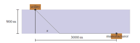
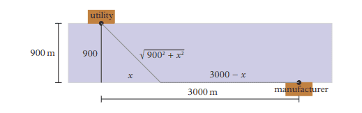
(1) We draw a picture of a utility on the bank of a straight river, with a manufacturer on the opposite side of the river but downstream. We also label the width of the river $(900 \mathrm{~m})$ and the downstream distance to the manufacturer $(3000 \mathrm{~m})$. See figure 9. Visualizing different possibilities, we see the pipeline could go straight to the opposite shore to have the least amount of pipe under water (figure 10 , top). The pipeline could also go directly to the manufacturer, remaining under water the entire route, to have the least total amount of pipe (figure 10 , bottom). But we are not asked to minimize the amount of pipe under water or minimize the total length of pipe; instead, we are asked to minimize cost. It seems as if the least cost prompts us to follow a route like that in figure 9.
(2) The variable amount in figure 9 appears to be the spot at which the pipe emerges from the river, which is in fact what we are asked for. Let’s let $x$ represent the distance downstream from the utility at which the pipe emerges, and label this distance in the diagram; see figure 11 . We can then determine and label other lengths as well. The length of the pipe along the shore is $(3000-x) \mathrm{m}$, whereas the “vertical leg” of the right triangle is the width of the river, $900 \mathrm{~m}$. The length of the hypotenuse can be found using the Pythagorean theorem: $c^2=$ $900^2+x^2$, or $c=\sqrt{900^2+x^2}$. These are labeled in figure 12 .
(3) The quantity we are asked to optimize (minimize in this case) is the cost of the pipeline. The cost of the pipeline includes the cost of running pipe under the water and the cost of running pipe along the shoreline. Under water, the pipeline cost is $\$ 200 / \mathrm{m}$, and from the diagram we see that the length of pipe under the water is $\sqrt{900^2+x^2} \mathrm{~m}$. Therefore, the cost of the pipe under the water is
$$
200 \sqrt{900^2+x^2}
$$
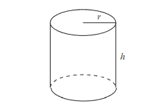
Example 5 A cylindrical can must have volume $100 \mathrm{~cm}^3$. What dimensions should be used to minimize the amount of material used?
Solution We notice the phrase “minimize the amount of material used” and conclude that this is an optimization problem.
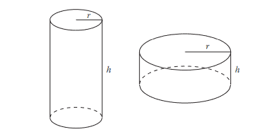
(1)-2) We are told the can is cylindrical, so we draw a cylindrical can (figure 13). We are asked for the dimensions to use, which include the can’s height and radius, so we visualize various possible shapes, such as tall and thin or short and wide (figure 14).
(3) We wish to minimize the amount of material used to make the can. The material of the can includes the top, bottom, and side of the can. Assuming a uniform thickness of the material, the material used is proportional to the surface area of the can. The formula for the surface area (SA) of a cylinder is
$$
S A=2 \pi r h+2 \pi r^2 .
$$
微积分代考
数学代写|微积分代写Calculus代写|Optimization example: maximum profit
回想一下,对于经济学中的收入、成本和利润函数,边际意味着”导数”。还记得利润是收入减去成本:
$$
P(x)=R(x)-C(x) .
$$
如果我们㹷望利润最大化,那么我们需要找到利润函数的临界数一一即 $P^{\prime}(x)=0$ :
$$
P^{\prime}(x)=R^{\prime}(x)-C^{\prime}(x) R^{\prime}(x)-C^{\prime}(x) \quad=0 R^{\prime}(x)=C^{\prime}(x)
$$
换句话说,利润函数的临界值出现在边际收益等于边际成本的地方。利润最大化问题的传统求解方法是使 边际收益与边际成本相等。因为我们还㹷望检查以确保利润最大化而不是最小化,所以我们仍然形成利润 函数并确定其最大值。
示例 4 每个月我们可以销售尽可能多的小部件 $\$ 12$ 每个。制造成本,以美元计 $x$ 小部件由
$$
C(x)=10000+7 x-0.002 x^2+\frac{1}{3} \cdot 10^{-6} x^3 .
$$
我们应该制作多少小部件才能使利润最大化?
解决方案 因为我们布望利润最大化,所以这是一个优化问题。
1)-2 请注意,此问题与几何无关。似乎没有图片适用,所以我们不画一张。此外,已经引入了相关变量; $x$ 是 1 个月内制作的小部件数量。
数学代写|微积分代写Calculus代写|Optimization example: minimum material
解决方案 首先我们认识到这是一个优化问题,因为我们被要求最小化成本。
(1) 我们在一条笔直的河岸上画了一个公用事业公司的图片,在河的对面下游有一个制造商。我们还标注 了河流的宽度 $(900 \mathrm{~m})$ 以及到制造商的下游距离 $(3000 \mathrm{~m})$. 参见图 9。可视化不同的可能性,我们看到 管道可以直接通向对岸,从而使水下管道数量最少(图 10,顶部)。管道也可以直接通向制造商,在整 个路线中保持在水下,以获得最少的管道总量(图 10,底部)。但我们并没有要求我们尽量减少水下管 道的数量或尽量减少管道的总长度;相反,我们被要求最小化成本。似乎最低成本促使我们遵循图 9 中 的路线。
(2) 图 9 中的变量似平是管道从河流中露出的位置,这实际上是我们所要求的。让我们让 $x$ 代表公用设施 下游管道出现的距离,并在图中标出该距离;见图 11。然后我们也可以确定和标记其他长度。沿岸管道 的长度为 $(3000-x) \mathrm{m}$ ,而直角三角形的“垂直边”是河流的宽度, $900 \mathrm{~m}$. 可以使用毕达哥拉斯定理找 到斜边的长度: $c^2=900^2+x^2$ , 要么 $c=\sqrt{900^2+x^2}$. 这些在图 12 中进行了标记。
(3) 我们被要求优化的数量(在这种情况下最小化) 是管道的成本。管道成本包括在水下铺设管道的成本 和沿海岸线铺设管道的成本。在水下,管道成本为 $\$ 200 / \mathrm{m}$ ,从图中我们可以看出水下管道的长度是 $\sqrt{900^2+x^2} \mathrm{~m}$. 因此,水下管道的造价为
$$
200 \sqrt{900^2+x^2}
$$
例 5 圆柱罐一定有体积 $100 \mathrm{~cm}^3$. 应该使用什么尺寸来最小化材料的使用量?
解决方案 我们注意到短语“最小化材料使用量”并得出结论,这是一个优化问题。
(1)-2) 我们被告知罐子是圆柱形的,所以我们画一个圆柱形罐头 (图13)。我们被要求提供要使用的尺 寸,其中包括罐头的高度和半径,因此我们想象出各种可能的形状,例如又高又薄或又短又宽(图
14)。
(3)我们莃望尽量减少制造罐头所用的材料量。罐的材料包括罐的顶部、底部和侧面。假设材料厚度均 匀,则所用材料与罐的表面积成正比。圆柱表面积 (SA) 的公式为
$$
S A=2 \pi r h+2 \pi r^2 .
$$

统计代写请认准statistics-lab™. statistics-lab™为您的留学生涯保驾护航。
金融工程代写
金融工程是使用数学技术来解决金融问题。金融工程使用计算机科学、统计学、经济学和应用数学领域的工具和知识来解决当前的金融问题,以及设计新的和创新的金融产品。
非参数统计代写
非参数统计指的是一种统计方法,其中不假设数据来自于由少数参数决定的规定模型;这种模型的例子包括正态分布模型和线性回归模型。
广义线性模型代考
广义线性模型(GLM)归属统计学领域,是一种应用灵活的线性回归模型。该模型允许因变量的偏差分布有除了正态分布之外的其它分布。
术语 广义线性模型(GLM)通常是指给定连续和/或分类预测因素的连续响应变量的常规线性回归模型。它包括多元线性回归,以及方差分析和方差分析(仅含固定效应)。
有限元方法代写
有限元方法(FEM)是一种流行的方法,用于数值解决工程和数学建模中出现的微分方程。典型的问题领域包括结构分析、传热、流体流动、质量运输和电磁势等传统领域。
有限元是一种通用的数值方法,用于解决两个或三个空间变量的偏微分方程(即一些边界值问题)。为了解决一个问题,有限元将一个大系统细分为更小、更简单的部分,称为有限元。这是通过在空间维度上的特定空间离散化来实现的,它是通过构建对象的网格来实现的:用于求解的数值域,它有有限数量的点。边界值问题的有限元方法表述最终导致一个代数方程组。该方法在域上对未知函数进行逼近。[1] 然后将模拟这些有限元的简单方程组合成一个更大的方程系统,以模拟整个问题。然后,有限元通过变化微积分使相关的误差函数最小化来逼近一个解决方案。
tatistics-lab作为专业的留学生服务机构,多年来已为美国、英国、加拿大、澳洲等留学热门地的学生提供专业的学术服务,包括但不限于Essay代写,Assignment代写,Dissertation代写,Report代写,小组作业代写,Proposal代写,Paper代写,Presentation代写,计算机作业代写,论文修改和润色,网课代做,exam代考等等。写作范围涵盖高中,本科,研究生等海外留学全阶段,辐射金融,经济学,会计学,审计学,管理学等全球99%专业科目。写作团队既有专业英语母语作者,也有海外名校硕博留学生,每位写作老师都拥有过硬的语言能力,专业的学科背景和学术写作经验。我们承诺100%原创,100%专业,100%准时,100%满意。
随机分析代写
随机微积分是数学的一个分支,对随机过程进行操作。它允许为随机过程的积分定义一个关于随机过程的一致的积分理论。这个领域是由日本数学家伊藤清在第二次世界大战期间创建并开始的。
时间序列分析代写
随机过程,是依赖于参数的一组随机变量的全体,参数通常是时间。 随机变量是随机现象的数量表现,其时间序列是一组按照时间发生先后顺序进行排列的数据点序列。通常一组时间序列的时间间隔为一恒定值(如1秒,5分钟,12小时,7天,1年),因此时间序列可以作为离散时间数据进行分析处理。研究时间序列数据的意义在于现实中,往往需要研究某个事物其随时间发展变化的规律。这就需要通过研究该事物过去发展的历史记录,以得到其自身发展的规律。
回归分析代写
多元回归分析渐进(Multiple Regression Analysis Asymptotics)属于计量经济学领域,主要是一种数学上的统计分析方法,可以分析复杂情况下各影响因素的数学关系,在自然科学、社会和经济学等多个领域内应用广泛。
MATLAB代写
MATLAB 是一种用于技术计算的高性能语言。它将计算、可视化和编程集成在一个易于使用的环境中,其中问题和解决方案以熟悉的数学符号表示。典型用途包括:数学和计算算法开发建模、仿真和原型制作数据分析、探索和可视化科学和工程图形应用程序开发,包括图形用户界面构建MATLAB 是一个交互式系统,其基本数据元素是一个不需要维度的数组。这使您可以解决许多技术计算问题,尤其是那些具有矩阵和向量公式的问题,而只需用 C 或 Fortran 等标量非交互式语言编写程序所需的时间的一小部分。MATLAB 名称代表矩阵实验室。MATLAB 最初的编写目的是提供对由 LINPACK 和 EISPACK 项目开发的矩阵软件的轻松访问,这两个项目共同代表了矩阵计算软件的最新技术。MATLAB 经过多年的发展,得到了许多用户的投入。在大学环境中,它是数学、工程和科学入门和高级课程的标准教学工具。在工业领域,MATLAB 是高效研究、开发和分析的首选工具。MATLAB 具有一系列称为工具箱的特定于应用程序的解决方案。对于大多数 MATLAB 用户来说非常重要,工具箱允许您学习和应用专业技术。工具箱是 MATLAB 函数(M 文件)的综合集合,可扩展 MATLAB 环境以解决特定类别的问题。可用工具箱的领域包括信号处理、控制系统、神经网络、模糊逻辑、小波、仿真等。