标签： MTH 3002

数学代写|拓扑学代写Topology代考|SETS AND SET INCLUSION

Posted on 2023年4月14日2023年4月14日 by statistics-lab

如果你也在怎样代写拓扑学Topology这个学科遇到相关的难题，请随时右上角联系我们的24/7代写客服。

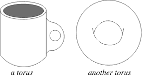
拓扑学是数学的一个分支，有时被称为 “橡胶板几何”，在这个分支中，如果两个物体可以通过弯曲、扭曲、拉伸和收缩等空间运动连续变形为彼此，同时不允许撕开或粘在一起的部分，则被认为是等效的。

statistics-lab™ 为您的留学生涯保驾护航在代写拓扑学Topology方面已经树立了自己的口碑, 保证靠谱, 高质且原创的统计Statistics代写服务。我们的专家在代写拓扑学Topology代写方面经验极为丰富，各种代写拓扑学Topology相关的作业也就用不着说。

我们提供的拓扑学Topology及其相关学科的代写，服务范围广, 其中包括但不限于:

Statistical Inference 统计推断
Statistical Computing 统计计算
Advanced Probability Theory 高等概率论
Advanced Mathematical Statistics 高等数理统计学
(Generalized) Linear Models 广义线性模型
Statistical Machine Learning 统计机器学习
Longitudinal Data Analysis 纵向数据分析
Foundations of Data Science 数据科学基础

数学代写|拓扑学代写Topology代考|SETS AND SET INCLUSION

We adopt a naive point of view in our discussion of sets and assume that the concepts of an element and of a set of elements are intuitively clear. By an element we mean an object or entity of some sort, as, for example, a positive integer, a point on the real line (= a real number), or a point in the complex plane ( = a complex number). A set is a collection or aggregate of such elements, considered together or as a whole. Some examples are furnished by the set of all even positive integers, the set of all rational points on the real line, and the set of all points in the complex plane whose distance from the origin is 1 (= the unit circle in the plane). We reserve the word class to refer to a set of sets. We might speak, for instance, of the class of all circles in a plane (thinking of each circle as a set of points). It will be useful in the work we do if we carry this hierarchy one step further and use the term family for a set of classes. One more remark: the words element, set, class, and family are not intended to be rigidly fixed in their usage; we use them fluidly, to express varying attitudes toward the mathematical objects and systems we study. It is entirely reasonable, for instance, to think of a circle not as a set of points, but as a single entity in itself, in which case we might justifiably speak of the set of all circles in a plane.

There are two standard notations available for designating a particular set. Whenever it is feasible to do so, we can list its elements between braces. Thus ${1,2,3}$ signifies the set consisting of the first three positive integers, ${1, i,-1,-i}$ is the set of the four fourth roots of unity, and ${ \pm 1, \pm 3, \pm 5, \ldots}$ is the set of all odd integers. This manner of specifying a set, by listing its elements, is unworkable in many circumstances. We are then obliged to fall back on the second method, which is to use a property or attribute that characterizes the elements of the set in question. If $P$ denotes a certain property of elements, then ${x: P}$ stands for the set of all elements $x$ for which the property $P$ is meaningful and true.

数学代写|拓扑学代写Topology代考|PARTITIONS AND EQUIVALENCE RELATIONS

In the first part of this section we consider a non-empty set $X$, and we study decompositions of $X$ into non-empty subsets which fill it out and have no elements in common with one another. We give special attention to the tools (equivalence relations) which are normally used to generate such decompositions.

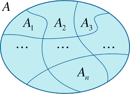
A partition of $X$ is a disjoint class $\left{X_i\right}$ of non-empty subsets of $X$ whose union is the full set $X$ itself. The $X_i$ ‘s are called the partition sets. Expressed somewhat differently, a partition of $X$ is the result of splitting it, or subdividing it, into non-empty subsets in such a way that each element of $X$ belongs to one and only one of the given subsets.

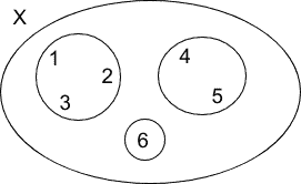
If $X$ is the set ${1,2,3,4,5}$, then ${1,3,5},{2,4}$ and ${1,2,3},{4,5}$ are two different partitions of $X$. If $X$ is the set $R$ of all real numbers, then we can partition $X$ into the set of all rationals and the set of all irrationals, or into the infinitely many closed-open intervals of the form $[n, n+1)$ where $n$ is an integer. If $X$ is the set of all points in the coordinate plane, then we can partition $X$ in such a way that each partition set consists of all points with the same $x$ coordinate (vertical lines), or so that each partition set consists of all points with the same $y$ coordinate (horizontal lines).

Other partitions of each of these sets will readily occur to the reader. In general, there are many different ways in which any given set can be partitioned. These manufactured examples are admittedly rather uninspiring and serve only to make our ideas more concrete. Later in this section we consider some others which are more germane to our present purposes.

A binary relation in the set $X$ is a mathematical symbol or verbal phrase, which we denote by $\mathrm{R}$ in this paragraph, such that for each ordered pair $(x, y)$ of elements of $X$ the statement $x \mathrm{R} y$ is meaningful, in the sense that it can be classified definitely as true or false. For such a binary relation, $x \mathrm{R} y$ symbolizes the assertion that $x$ is related by $\mathrm{R}$ to $y$, and $x \not R y$ the negation of this, namely, the assertion that $x$ is not related by $\mathrm{R}$ to $y$ Many examples of binary relations can be given, some familiar and others less so, some mathematical and others not. For instance, if $X$ is the set of all integers and $\mathrm{R}$ is interpreted to mean “is less than,” which of course is usually denoted by the symbol $<$, then we clearly have $4<7$ and $5 \nless 2$. We have been speaking of binary relations, which are so named because they apply only to ordered pairs of elements, rather than to ordered triples, etc. In our work we drop the qualifying adjective and speak simply of a relation in $X$, since we shall have occasion to consider only relations of this kind. ${ }^1$

拓扑学代考

数学代写|拓扑学代写Topology代考|SETS AND SET INCLUSION

我们在讨论集合时采用了一种朴素的观点，并假设一个元素和一组元素的概念在直觉上是清楚的。我们所说的元素是指某种对象或实体，例如正整数、实线上的点（= 实数）或复平面中的点（= 复数）。集合是这些元素的集合或聚合，一起或作为一个整体来考虑。一些例子由所有偶数正整数的集合，实线上所有有理点的集合，以及复平面中距离原点为1（=平面中的单位圆）的所有点的集合提供。 . 我们保留单词类来指代一组集合。例如，我们可以谈论平面上所有圆的类（将每个圆视为一组点）。如果我们将此层次结构更进一步并使用术语系列来表示一组类，这将对我们所做的工作很有用。还有一点要注意：元素、集合、类和族这些词并不是要严格固定在它们的用法中；我们流畅地使用它们来表达对我们研究的数学对象和系统的不同态度。例如，不把一个圆看作一组点，而是把它看作一个单独的实体是完全合理的，在这种情况下，我们可以合理地谈论一个平面上所有圆的集合。

有两种标准符号可用于指定特定集合。只要可行，我们就可以在大括号之间列出它的元素。因此1,2,3表示由前三个正整数组成的集合，1,我,−1,−我是四次单位根的集合，并且±1,±3,±5,…是所有奇数的集合。这种通过列出其元素来指定集合的方式在许多情况下是行不通的。然后我们不得不求助于第二种方法，即使用表征所讨论集合元素的特性或属性。如果P表示元素的某个属性，则X:P代表所有元素的集合X为哪个财产P是有意义和真实的。

数学代写|拓扑学代写Topology代考|PARTITIONS AND EQUIVALENCE RELATIONS

在本节的第一部分，我们考虑一个非空集X，我们研究分解X成非空子集，这些子集填充它并且彼此没有共同的元素。我们特别关注通常用于生成此类分解的工具（等价关系）。

的分区X是一个不相交的类\左{X_i\右}的非空子集X谁的联合是完整的X本身。这X我的称为分区集。表达方式略有不同，分区X是将其拆分或细分为非空子集的结果，其中的每个元素X属于一个且仅一个给定的子集。

如果X是集合1,2,3,4,5，然后1,3,5,2,4和1,2,3,4,5是两个不同的分区X. 如果X是集合R的所有实数，那么我们可以划分X进入所有有理数的集合和所有无理数的集合，或进入形式的无限多个闭-开区间[n,n+1)在哪里n是一个整数。如果X是坐标平面内所有点的集合，那么我们可以划分X以这样的方式，每个分区集由具有相同的所有点组成X坐标（垂直线），或者使每个分区集由具有相同特征的所有点组成和坐标（水平线）。

读者很容易想到这些集合中的每一个的其他分区。一般来说，任何给定的集合都可以有多种不同的划分方式。诚然，这些制造的例子相当乏味，只能使我们的想法更加具体。在本节的后面，我们将考虑一些与我们目前的目的更相关的其他内容。

集合中的二元关系X是一个数学符号或口头短语，我们用R在本段中，对于每个有序对(X,和)的元素X该声明XR和是有意义的，因为它可以明确地分类为真或假。对于这样的二元关系，XR和象征着断言X与R到和，和XR 和对此的否定，即断言X与以下无关R到和可以给出许多二元关系的例子，有些很熟悉，有些不太熟悉，有些是数学的，有些则不是。例如，如果X是所有整数的集合，并且R被解释为“小于”，当然通常用符号表示<, 那么我们显然有4<7和5≮2. 我们一直在谈论二元关系，之所以这样命名，是因为它们仅适用于有序的元素对，而不适用于有序的三元组等。在我们的工作中，我们放弃了限定形容词，而简单地谈论关系X，因为我们将有机会只考虑这种关系。

统计代写请认准statistics-lab™. statistics-lab™为您的留学生涯保驾护航。

金融工程代写

金融工程是使用数学技术来解决金融问题。金融工程使用计算机科学、统计学、经济学和应用数学领域的工具和知识来解决当前的金融问题，以及设计新的和创新的金融产品。

非参数统计代写

非参数统计指的是一种统计方法，其中不假设数据来自于由少数参数决定的规定模型；这种模型的例子包括正态分布模型和线性回归模型。

广义线性模型代考

广义线性模型（GLM）归属统计学领域，是一种应用灵活的线性回归模型。该模型允许因变量的偏差分布有除了正态分布之外的其它分布。

术语广义线性模型（GLM）通常是指给定连续和/或分类预测因素的连续响应变量的常规线性回归模型。它包括多元线性回归，以及方差分析和方差分析（仅含固定效应）。

有限元方法代写

有限元方法（FEM）是一种流行的方法，用于数值解决工程和数学建模中出现的微分方程。典型的问题领域包括结构分析、传热、流体流动、质量运输和电磁势等传统领域。

有限元是一种通用的数值方法，用于解决两个或三个空间变量的偏微分方程（即一些边界值问题）。为了解决一个问题，有限元将一个大系统细分为更小、更简单的部分，称为有限元。这是通过在空间维度上的特定空间离散化来实现的，它是通过构建对象的网格来实现的：用于求解的数值域，它有有限数量的点。边界值问题的有限元方法表述最终导致一个代数方程组。该方法在域上对未知函数进行逼近。[1] 然后将模拟这些有限元的简单方程组合成一个更大的方程系统，以模拟整个问题。然后，有限元通过变化微积分使相关的误差函数最小化来逼近一个解决方案。

tatistics-lab作为专业的留学生服务机构，多年来已为美国、英国、加拿大、澳洲等留学热门地的学生提供专业的学术服务，包括但不限于Essay代写，Assignment代写，Dissertation代写，Report代写，小组作业代写，Proposal代写，Paper代写，Presentation代写，计算机作业代写，论文修改和润色，网课代做，exam代考等等。写作范围涵盖高中，本科，研究生等海外留学全阶段，辐射金融，经济学，会计学，审计学，管理学等全球99%专业科目。写作团队既有专业英语母语作者，也有海外名校硕博留学生，每位写作老师都拥有过硬的语言能力，专业的学科背景和学术写作经验。我们承诺100%原创，100%专业，100%准时，100%满意。

随机分析代写

随机微积分是数学的一个分支，对随机过程进行操作。它允许为随机过程的积分定义一个关于随机过程的一致的积分理论。这个领域是由日本数学家伊藤清在第二次世界大战期间创建并开始的。

时间序列分析代写

随机过程，是依赖于参数的一组随机变量的全体，参数通常是时间。随机变量是随机现象的数量表现，其时间序列是一组按照时间发生先后顺序进行排列的数据点序列。通常一组时间序列的时间间隔为一恒定值（如1秒，5分钟，12小时，7天，1年），因此时间序列可以作为离散时间数据进行分析处理。研究时间序列数据的意义在于现实中，往往需要研究某个事物其随时间发展变化的规律。这就需要通过研究该事物过去发展的历史记录，以得到其自身发展的规律。

回归分析代写

多元回归分析渐进（Multiple Regression Analysis Asymptotics）属于计量经济学领域，主要是一种数学上的统计分析方法，可以分析复杂情况下各影响因素的数学关系，在自然科学、社会和经济学等多个领域内应用广泛。

MATLAB代写

MATLAB 是一种用于技术计算的高性能语言。它将计算、可视化和编程集成在一个易于使用的环境中，其中问题和解决方案以熟悉的数学符号表示。典型用途包括：数学和计算算法开发建模、仿真和原型制作数据分析、探索和可视化科学和工程图形应用程序开发，包括图形用户界面构建MATLAB 是一个交互式系统，其基本数据元素是一个不需要维度的数组。这使您可以解决许多技术计算问题，尤其是那些具有矩阵和向量公式的问题，而只需用 C 或 Fortran 等标量非交互式语言编写程序所需的时间的一小部分。MATLAB 名称代表矩阵实验室。MATLAB 最初的编写目的是提供对由 LINPACK 和 EISPACK 项目开发的矩阵软件的轻松访问，这两个项目共同代表了矩阵计算软件的最新技术。MATLAB 经过多年的发展，得到了许多用户的投入。在大学环境中，它是数学、工程和科学入门和高级课程的标准教学工具。在工业领域，MATLAB 是高效研究、开发和分析的首选工具。MATLAB 具有一系列称为工具箱的特定于应用程序的解决方案。对于大多数 MATLAB 用户来说非常重要，工具箱允许您学习和应用专业技术。工具箱是 MATLAB 函数（M 文件）的综合集合，可扩展 MATLAB 环境以解决特定类别的问题。可用工具箱的领域包括信号处理、控制系统、神经网络、模糊逻辑、小波、仿真等。

R语言代写	问卷设计与分析代写
PYTHON代写	回归分析与线性模型代写
MATLAB代写	方差分析与试验设计代写
STATA代写	机器学习/统计学习代写
SPSS代写	计量经济学代写
EVIEWS代写	时间序列分析代写
EXCEL代写	深度学习代写
SQL代写	各种数据建模与可视化代写

数学代写|拓扑学代写Topology代考|MATH6204

Posted on 2023年3月1日2023年3月1日 by statistics-lab

如果你也在怎样代写拓扑学Topology这个学科遇到相关的难题，请随时右上角联系我们的24/7代写客服。

我们提供的拓扑学Topology及其相关学科的代写，服务范围广, 其中包括但不限于:

Statistical Inference 统计推断
Statistical Computing 统计计算
Advanced Probability Theory 高等概率论
Advanced Mathematical Statistics 高等数理统计学
(Generalized) Linear Models 广义线性模型
Statistical Machine Learning 统计机器学习
Longitudinal Data Analysis 纵向数据分析
Foundations of Data Science 数据科学基础

数学代写|拓扑学代写Topology代考|Subspaces

A subset of a space inherits a topology from its parent space, in an obvious way. This is the simplest method of constructing a new space from a given one.

Definition 1.5.1 Let $(X, \mathscr{T})$ be a space and $Y \subseteq X$. The relative topology or the subspace topology $\mathscr{T}_Y$ on $Y$ is the collection of all intersections of $Y$ with open subsets of $X$, and $Y$ equipped with this topology is called a subspace of $X$.

A routine verification shows that $\mathscr{T}_Y={Y \cap U \mid U \in \mathscr{T}}$ is, indeed, a topology on $Y$. Each member $H$ of $\mathscr{T}_Y$ is said to be open in $Y$ and its relative complement $Y-H$ is closed in $Y$. We have the following

Proposition 1.5.2 Let $Y$ be a subspace of a space $X$. A subset $K \subseteq Y$ is closed in $Y$ if and only if $K=Y \cap F$, where $F$ is closed in $X$.

Proof For any $F \subseteq X$, we have $Y-(Y \cap F)=Y \cap(X-F)$, and it follows that $K$ is closed in $Y$ if $K=Y \cap F$ and $F$ is closed in $X$. Conversely, suppose that $K$ is closed in $Y$. Then $Y-K=Y \cap G$ for an open subset $G$ of $X$. This implies that $K=Y \cap(X-G)$, where $X-G$ is obviously closed in $X$.

Example 1.5.1 Let $(X, d)$ be a metric space and $Y \subseteq X$. Then the relative topology on $Y$ induced by the metric topology on $X$ coincides with the metric topology determined by the restriction of $d$ to $Y$. This follows from the observation that an open ball about $y$ of radius $r$ in $Y$ is the intersection of $Y$ with the open ball $B(y ; r)$ in $X$. In particular, we see that $\mathbb{D}^n, I^n$ and $\mathbb{S}^{n-1}$ have the same topological structures whether considered as subspaces of the Euclidean metric space $\mathbb{R}^n$ or those of the space $\mathbb{R}^n$ with the usual topology.

If $Y$ is a subspace of $X$, then any subset of $Y$ which is open (or closed) in $X$ has the same property in $Y$. But, an open (or closed) subset of $Y$ need not be open (or closed) in $X$, as shown by the following.

Example 1.5.2 In the subspace $Y=(0,1] \cup[2,3]$ of $\mathbb{R}$, the set $(0,1]$ is open as well as closed. But this is not open or closed in $\mathbb{R}$.
In this regard, we have the following.
Proposition 1.5.3 Let $Y$ be a subspace of a space $X$. If $Y$ is closed (or open) in $X$ and $A$ is closed (resp. open) in $Y$, then $A$ is closed (resp. open) in $X$.

数学代写|拓扑学代写Topology代考|Continuous Functions

The conditions of a topological structure have been so formulated that the definition of a continuous function can be borrowed word for word from analysis.

Definition 2.1.1 Let $X$ and $Y$ be spaces. A function $f: X \rightarrow Y$ is called continuous if $f^{-1}(U)$ is open in $X$ for each open set $U \subseteq Y$.

Example 2.1.1 A constant function $c: X \rightarrow Y$ is obviously continuous, for $c^{-1}(U)$ is either $\varnothing$ or $X$ for every $U \subseteq Y$.
Example 2.1.2 Every function on a discrete space is continuous.
The following theorem provides some other ways of formulating the continuity condition.

Theorem 2.1.2 Let $X$ and $Y$ be topological spaces, and let $f: X \rightarrow Y$ be a function. The following conditions are equivalent:
(a) $f$ is continuous.
(b) $f^{-1}(F)$ is closed in $X$ for every closed set $F \subseteq Y$.

(c) $f(\bar{A}) \subseteq \overline{f(A)}$ for every set $A \subseteq X$.
(d) $\overline{f^{-1}(B)} \subseteq f^{-1}(\bar{B})$ for every set $B \subseteq Y$.
Proof (a) $\Leftrightarrow$ (b): This is immediate from the equality $f^{-1}(Y-B)=X-f^{-1}(B)$.
Now, we prove that (b) $\Rightarrow$ (c) $\Rightarrow$ (d) $\Rightarrow$ (b).
(b) $\Rightarrow$ (c): Since $\overline{f(A)}$ is closed, $f^{-1}(\overline{f(A)})$ is closed, by (b). Obviously, $A \subseteq$ $f^{-1}(\overline{f(A)})$; so $\bar{A} \subseteq f^{-1}(\overline{f(A)})$ and $(c)$ holds.
(c) $\Rightarrow$ (d): Taking $A=f^{-1}(B)$ in $(c)$, we have $f\left(\overline{f^{-1}(B)}\right) \subseteq \overline{f\left(f^{-1}(B)\right)} \subseteq \bar{B}$, which implies $(d)$.
(d) $\Rightarrow$ (b): If $F$ is a closed subset of $Y$, then $(d)$ implies $\overline{f^{-1}(F)} \subseteq f^{-1}(F)$. But $f^{-1}(F) \subseteq \overline{f^{-1}(F)}$ always, so the equality holds and $f^{-1}(F)$ is closed.

If a basis (or subbasis) for a space $Y$ is known, then the task of proving the continuity of a function into $Y$ becomes easier, as shown by the following.

拓扑学代考

数学代写|拓扑学代写Topology代考|Subspaces

空间的子集以一种显而易见的方式从其父空间继承拓扑。这是从给定空间构造新空间的最简单方法。
定义 1.5.1 让 $(X, \mathscr{T})$ 是一个空间和 $Y \subseteq X$. 相对拓扑或子空间拓扑 $\mathscr{T}_Y$ 在 $Y$ 是所有交集的集合 $Y$ 的开放子集 $X$ ，和 $Y$ 配备此拓扑的子空间称为 $X$.
例行验证表明 $\mathscr{T}_Y=Y \cap U \mid U \in \mathscr{T}$ 确实是一个拓扑 $Y$. 每个成员 $H$ 的 $\mathscr{T}_Y$ 据说开在 $Y$ 及其相对补语 $Y-H$ 关闭于 $Y$. 我们有以下
命题 1.5.2 让 $Y$ 是空间的子空间 $X$.一个子集 $K \subseteq Y$ 关闭于 $Y$ 当且仅当 $K=Y \cap F$ ，在哪里 $F$ 关闭于 $X$.
证明对于任何 $F \subseteq X$ ，我们有 $Y-(Y \cap F)=Y \cap(X-F)$ ，它遵循 $K$ 关闭于 $Y$ 如果 $K=Y \cap F$ 和 $F$ 关闭于 $X$. 相反，假设 $K$ 关闭于 $Y$. 然后 $Y-K=Y \cap G$ 对于一个开放子集 $G$ 的 $X$. 这意味着 $K=Y \cap(X-G) ，$ 在哪里 $X-G$ 显然是封闭的 $X$.
示例 1.5.1 让 $(X, d)$ 是一个度量空间并且 $Y \subseteq X$. 然后是相对拓扑 $Y$ 由度量拓扑引起 $X$ 符合由限制确定的度量拓扑 $d$ 到 $Y$. 这是从观察到一个开放的球大约 $y$ 半径 $r$ 在 $Y$ 是交集 $Y$ 用开球 $B(y ; r)$ 在 $X$. 特别地，我们看到 $\mathbb{D}^n, I^n$ 和 $\mathbb{S}^{n-1}$ 无论是否被视为欧几里得度量空间的子空间，都具有相同的拓扑结构 $\mathbb{R}^n$ 或那些空间 $\mathbb{R}^n$ 与通常的拓扑结构。
如果 $Y$ 是一个子空间 $X$ ，那么任何子集 $Y$ 这是开放的（或封闭的) $X$ 拥有相同的财产 $Y$. 但是，一个开放 (或封闭) 的子集 $Y$ 不需要打开（或关闭) $X$ ，如下图所示。
例 1.5.2 在子空间 $Y=(0,1] \cup[2,3]$ 的 $\mathbb{R}$ ，集合 $(0,1]$ 是开放的也是封闭的。但这不是开放或关闭的 $\mathbb{R}$. 对此，我们有以下几点。
命题 1.5.3 让 $Y$ 是空间的子空间 $X$. 如果 $Y$ 关闭 (或打开) 于 $X$ 和 $A$ 关闭 (分别打开) $Y$ ，然后 $A$ 关闭 (分别打开) $X$.

数学代写|拓扑学代写Topology代考|Continuous Functions

拓扑结构的条件已经制定，连续函数的定义可以从分析中逐字借用。
定义 2.1.1 让 $X$ 和 $Y$ 是空格。一个函数 $f: X \rightarrow Y$ 称为连续的如果 $f^{-1}(U)$ 打开于 $X$ 对于每个开集 $U \subset Y$
示例 2.1.1 常量函数 $c: X \rightarrow Y$ 显然是连续的，因为 $c^{-1}(U)$ 或者是 $\varnothing$ 或者 $X$ 每一个 $U \subseteq Y$.
示例 $2.1 .2$ 离散空间上的每个函数都是连续的。
下面的定理提供了表达连续性条件的其他一些方法。
定理 2.1.2 让 $X$ 和 $Y$ 是拓扑空间，让 $f: X \rightarrow Y$ 成为一个函数。以下条件是等效的:
(a) $f$ 是连续的。
(二) $f^{-1}(F)$ 关闭于 $X$ 对于每个闭集 $F \subseteq Y$.
(C) $f(\bar{A}) \subseteq \overline{f(A)}$ 每尝 $A \subseteq X$.
(四) $\overline{f^{-1}(B)} \subseteq f^{-1}(\bar{B})$ 每套 $B \subseteq Y$.
证明 $(一) \Leftrightarrow(b)$ : 这是直接从平等 $f^{-1}(Y-B)=X-f^{-1}(B)$.
现在，我们证明 $(b) \Rightarrow(C) \Rightarrow($ 四 $) \Rightarrow($ 二 $)$.
(二) $\Rightarrow(c)$ : 因为 $\overline{f(A)}$ 关闭了， $f^{-1}(\overline{f(A)})$ 由 (b) 关闭。明显地， $A \subseteq f^{-1}(\overline{f(A)})$; 所以 $\bar{A} \subseteq f^{-1}(\overline{f(A)})$ 和 $(c)$ 持有。
$(C) \Rightarrow(\mathrm{d})$ : 服用 $A=f^{-1}(B)$ 在 $(c)$ ，我们有 $f\left(\overline{f^{-1}(B)}\right) \subseteq \overline{f\left(f^{-1}(B)\right)} \subseteq \bar{B}$ ，这意味着 $(d)$.
$($ 四 $) \Rightarrow(\mathrm{b})$ : 如果 $F$ 是的闭子集 $Y$ ，然后 $(d)$ 暗示 $\overline{f^{-1}(F)} \subseteq f^{-1}(F)$. 但 $f^{-1}(F) \subseteq \overline{f^{-1}(F)}$ 总是，所以等式成立并且 $f^{-1}(F)$ 关闭了。
如果一个空间的基 (或子基) $Y$ 已知，则证明函数连续性的任务为 $Y$ 变得更容易，如下所示。

统计代写请认准statistics-lab™. statistics-lab™为您的留学生涯保驾护航。

金融工程代写

非参数统计代写

非参数统计指的是一种统计方法，其中不假设数据来自于由少数参数决定的规定模型；这种模型的例子包括正态分布模型和线性回归模型。

广义线性模型代考

广义线性模型（GLM）归属统计学领域，是一种应用灵活的线性回归模型。该模型允许因变量的偏差分布有除了正态分布之外的其它分布。

有限元方法代写

随机分析代写

时间序列分析代写

回归分析代写

MATLAB代写

R语言代写	问卷设计与分析代写
PYTHON代写	回归分析与线性模型代写
MATLAB代写	方差分析与试验设计代写
STATA代写	机器学习/统计学习代写
SPSS代写	计量经济学代写
EVIEWS代写	时间序列分析代写
EXCEL代写	深度学习代写
SQL代写	各种数据建模与可视化代写

数学代写|拓扑学代写Topology代考|MTH3130

Posted on 2023年3月1日2023年3月1日 by statistics-lab

如果你也在怎样代写拓扑学Topology这个学科遇到相关的难题，请随时右上角联系我们的24/7代写客服。

我们提供的拓扑学Topology及其相关学科的代写，服务范围广, 其中包括但不限于:

Statistical Inference 统计推断
Statistical Computing 统计计算
Advanced Probability Theory 高等概率论
Advanced Mathematical Statistics 高等数理统计学
(Generalized) Linear Models 广义线性模型
Statistical Machine Learning 统计机器学习
Longitudinal Data Analysis 纵向数据分析
Foundations of Data Science 数据科学基础

数学代写|拓扑学代写Topology代考|Adjoint Analysis

Based on the Lagrangian multiplier-based adjoint method and the adjoint analysis of the transformed topology optimization problem in Eq. 2.21, the weak forms of the adjoint equations for the topology optimization problem in Eq. $2.15$ are derived as (the details are presented in Appendix 2.7.1):
Find $\hat{H}{s z}$ with $\operatorname{Re}\left(\hat{H}{s z}\right) \in \mathscr{H}\left(\Omega \cup \Omega_P\right), \operatorname{Im}\left(\hat{H}{s z}\right) \in \mathscr{H}\left(\Omega \cup \Omega_P\right)$ and $\hat{H}{s z}=0$ on $\Gamma_D$, such that
$$
\begin{aligned}
& \int_{\Omega}\left(\frac{\partial A}{\partial \operatorname{Re}\left(H_{s z}\right)}-j \frac{\partial A}{\partial \operatorname{Im}\left(H_{s z}\right)}\right) \phi+\left(\frac{\partial A}{\partial \nabla \operatorname{Re}\left(H_{s z}\right)}-j \frac{\partial A}{\partial \nabla \operatorname{Im}\left(H_{s z}\right)}\right) \cdot \nabla \phi \
& -\varepsilon_r^{-1} \nabla \hat{H}{s z}^* \cdot \nabla \phi+k_0^2 \mu_r \hat{H}{s z}^* \phi \mathrm{d} \Omega+\int_{\Omega_P}-\varepsilon_r^{-1}\left(\mathbf{T} \nabla \hat{H}{s z}^\right) \cdot(\mathbf{T} \nabla \phi)|\mathbf{T}|^{-1} \ & +k_0^2 \mu_r \hat{H}{s z}^ \phi|\mathbf{T}| \mathrm{d} \Omega=0, \forall \phi \in \mathscr{H}\left(\Omega \cup \Omega_P\right)
\end{aligned}
$$
and
Find $\hat{\gamma}f \in \mathscr{H}\left(\Omega_d\right)$ such that $$ \begin{aligned} & \int{\Omega_d} r^2 \nabla \hat{\gamma}f \cdot \nabla \varphi+\hat{\gamma}_f \varphi+\left[\sum{n=1}^N \frac{1}{V_n} \int_{P_n} \frac{\partial A}{\partial \gamma_p} \frac{\partial \gamma_p}{\partial \gamma_e}-\operatorname{Re}\left(\frac{\partial \varepsilon_r^{-1}}{\partial \gamma_p} \frac{\partial \gamma_p}{\partial \gamma_e} \nabla\left(H_{s z}+H_{i z}\right)\right)\right. \
& \left.\cdot \operatorname{Re}\left(\nabla \hat{H}{s z}^\right)+\operatorname{Im}\left(\frac{\partial \varepsilon_r^{-1}}{\partial \gamma_p} \frac{\partial \gamma_p}{\partial \gamma_e} \nabla\left(H{s z}+H_{i z}\right)\right) \cdot \operatorname{Im}\left(\nabla \hat{H}{s z}^\right) \mathrm{d} \Omega\right] \varphi \mathrm{d} \Omega=0 \
& \forall \varphi \in \mathscr{H}\left(\Omega_d\right),
\end{aligned}
$$
where $\hat{H}{s z}$ and $\hat{\gamma}f$ are the adjoint variables of $H{s z}$ and $\gamma_f$ respectively; ${ }^*$ is the operator used to implement the conjugate of a complex variable; $\Gamma_D$ is the perfect magnetic conductor boundary; $\mathscr{H}\left(\Omega \cup \Omega_P\right)$ and $\mathscr{H}\left(\Omega_d\right)$ are the first-order Hilbert spaces for the real functions defined on $\Omega \cup \Omega_P$ and $\Omega_d$ respectively; Re and $I m$ are operators used to extract the real and imaginary parts of a complex. The adjoint sensitivity is derived as
$$
\delta \hat{J}=\int_{\Omega_d}\left(\frac{\partial A}{\partial \gamma}-\hat{\gamma}_f\right) \delta \gamma \mathrm{d} \Omega, \forall \delta \gamma \in \mathscr{L}^2\left(\Omega_d\right)
$$

数学代写|拓扑学代写Topology代考|Numerical Implementation

The topology optimization problems are solved by a gradient-based iterative procedure, where the gradient information is derived by the self-consistent adjoint sensitivity. The flowchart for iterative solution of the optimization problems is shown in Fig. 2.2. The iterative procedure includes the following steps: (1) initialize the design variable and optimization parameters; (2) solve the wave equations with the current design variable and compute the value of the design objective; (3) solve the adjoint equations based on the solution of the wave equations; (4) compute the adjoint derivative of the design objective; (5) update the design variable using the method of moving asymptotes [20]; (6) do postprocessing, if the stopping criteria are satisfied, or else return to the step (2).

In this solution procedure, the filter radius $r$ of the PDE filter in Eq. $2.10$ is set to be $2 / 15$ of the incident wavelength; the threshold parameter $\xi$ in Eq. $2.12$ is set to be $0.5$; the initial value of the projection parameter $\beta$ is set to be 1 and it is doubled after every fixed number of iterations until the preset maximal value of $2^{10}$ is reached. The above steps are implemented iteratively until the stopping criteria are satisfied, and the stopping criteria are specified to be the maximal iteration number and the change of the objective values in five consecutive iterations satisfying
$$
\frac{1}{5} \sum_{i=1}^4\left|J_{k-i}-J_{k-i-1}\right| /\left|J_k\right| \leq \varepsilon, \beta \geq 2^{10}
$$
in the $k$ th iteration, where $J_k$ is the objective value computed in the $k$ th iteration; $\varepsilon$ is the tolerance chosen to be $1 \times 10^{-3}$.

In the iterative procedure, the numerical solution of PDEs are implemented based on finite element method $[10,13]$. The two-dimensional wave equation, the filter equation and the corresponding adjoint equations are solved using the standard Galerkin finite element method; the three-dimensional wave equation and the corresponding adjoint equation are solved using the edge element-based finite element method with linear edge elements $[14,15]$. It is noted that the original wave equations $2.1$ and $2.2$ are solved instead of the coupled equations for the split variables, because the sole destination of splitting operation is to derive the Fréchet differentiability during the adjoint analysis.

In the optimization procedures for the two-dimensional problems, the magnetic field, design variable and filtered design variable are interpolated using linear node elements (Fig. 2.3a); and the projected design variable is interpolated using zerothorder discontinuous elements (Fig. 2.3b). In the optimization procedure for the threedimensional problems, the electric field is interpolated using linear edge elements (Fig. 2.4a); the design variable and filtered design variable is interpolated using linear nodal elements (Fig. 2.4b); the filtered design variable is converted to piecewise form by interpolating the piecewise design variable using zeroth-order discontinuous elements (Fig. 2.4c), where $P_n$ in Eq. $2.11$ is set to be the space taken up by the finite elements.

拓扑学代考

数学代写|拓扑学代写Topology代考|Adjoint Analysis

基于基于拉格朗日乘数的伴随方法和方程中变换后的拓扑优化问题的伴随分析。2.21，方程中拓扑优化问题的伴随方程的弱形式。 $2.15$
推导为 (详情见附录 2.7.1) : $\hat{H} s z$ 和 $\operatorname{Re}(\hat{H} s z) \in \mathscr{H}\left(\Omega \cup \Omega_P\right), \operatorname{Im}(\hat{H} s z) \in \mathscr{H}\left(\Omega \cup \Omega_P\right)$ 和 $\hat{H} s z=0$ 在 $\Gamma_D$, 这样
并
找到 $\hat{\gamma} f \in \mathscr{H}\left(\Omega_d\right)$ 这样
在哪里 $\hat{H} s z$ 和 $\hat{\gamma} f$ 是伴随变量 $H s z$ 和 $\gamma_f$ 分别; ${ }^*$ 是用于实现复变量共轭的运算符； $\Gamma_D$ 是完美的磁导体边界； $\mathscr{H}\left(\Omega \cup \Omega_P\right)$ 和 $\mathscr{H}\left(\Omega_d\right)$ 是定义在上的实函数的一阶希尔伯特空间 $\Omega \cup \Omega_P$ 和 $\Omega_d$ 分别; 重新和 $I m$ 是用于提取复数的实部和虚部的运算符。伴随灵敏度推导为
$$
\delta \hat{J}=\int_{\Omega_d}\left(\frac{\partial A}{\partial \gamma}-\hat{\gamma}_f\right) \delta \gamma \mathrm{d} \Omega, \forall \delta \gamma \in \mathscr{L}^2\left(\Omega_d\right)
$$

数学代写|拓扑学代写Topology代考|Numerical Implementation

拓扑优化问题通过基于梯度的迭代过程解决，其中梯度信息由自洽伴随灵敏度导出。优化问题的迭代求解流程图如图 $2.2$ 所示。迭代过程包括以下步㡜：(1) 初始化设计变量和优化参数；(2) 用当前设计变量求解波动方程，计算设计目标值；(3) 在求解波动方程的基础上求解伴随方程；(4) 计算设计目标的伴随导数；(5) 采用移动渐近线的方法更新设计变量[20]；(6) 进行后处理，如果满足停止条件，则返回步㡜(2)。
在此求解过程中，滤波器半径 $r$ 等式中的 PDE 滤波器。 $2.10$ 被设置为 $2 / 15$ 入射波长；阈值参数 $\xi$ 在等式中 $2.12$ 被设置为 $0.5$; 投影参数的初始值 $\beta$ 设置为 1 ，每固定次数迭代后加倍，直到预设的最大值 $2^{10}$ 到达了。迭代执行上述步骤，直到满足停止准则，停止准则指定为最大迭代次数和连续五次迭代中目标值的变化满足
$$
\frac{1}{5} \sum_{i=1}^4\left|J_{k-i}-J_{k-i-1}\right| /\left|J_k\right| \leq \varepsilon, \beta \geq 2^{10}
$$
在里面 $k$ 第 th 次迭代，其中 $J_k$ 是在计算的目标值 $k$ 第次迭代； $\varepsilon$ 是公差选择是 $1 \times 10^{-3}$.
在迭代过程中，偏微分方程的数值解是基于有限元法实现的 $[10,13]$. 采用标准伽辽金有限元法求解二维波动方程、滤波器方程和相应的伴随方程; 三维波动方程和相应的伴随方程是使用基于边元的有限元方法求解的，具有线性边元 $[14,15]$. 值得注意的是，原始波动方程 $2.1$ 和 $2.2$ 求解，而不是拆分变量的耦合方程，因为拆分操作的唯一目的是在伴随分析期间导出 Fréchet 可微性。
在二维问题的优化程序中，磁场、设计变量和过滤后的设计变量使用线性节点元素进行揷值（图
2.3a）；并且使用零阶不连续元素对投影设计变量进行揷值 (图 2.3b) 。在三维问题的优化过程中，使用线性边缘元素对电场进行揷值（图 2.4a) ；使用线性节点元素对设计变量和过滤设计变量进行揷值
(图 2.4b) ；通过使用零阶不连续元素对分段设计变量进行揷值，将过滤后的设计变量转换为分段形式 (图 2.4c)，其中 $P_n$ 在等式中 $2.11$ 被设置为有限元占据的空间。

统计代写请认准statistics-lab™. statistics-lab™为您的留学生涯保驾护航。

金融工程代写

非参数统计代写

非参数统计指的是一种统计方法，其中不假设数据来自于由少数参数决定的规定模型；这种模型的例子包括正态分布模型和线性回归模型。

广义线性模型代考

广义线性模型（GLM）归属统计学领域，是一种应用灵活的线性回归模型。该模型允许因变量的偏差分布有除了正态分布之外的其它分布。

有限元方法代写

随机分析代写

时间序列分析代写

回归分析代写

MATLAB代写

R语言代写	问卷设计与分析代写
PYTHON代写	回归分析与线性模型代写
MATLAB代写	方差分析与试验设计代写
STATA代写	机器学习/统计学习代写
SPSS代写	计量经济学代写
EVIEWS代写	时间序列分析代写
EXCEL代写	深度学习代写
SQL代写	各种数据建模与可视化代写

数学代写|拓扑学代写Topology代考|MATH3402

Posted on 2023年3月1日2023年3月1日 by statistics-lab

如果你也在怎样代写拓扑学Topology这个学科遇到相关的难题，请随时右上角联系我们的24/7代写客服。

我们提供的拓扑学Topology及其相关学科的代写，服务范围广, 其中包括但不限于:

Statistical Inference 统计推断
Statistical Computing 统计计算
Advanced Probability Theory 高等概率论
Advanced Mathematical Statistics 高等数理统计学
(Generalized) Linear Models 广义线性模型
Statistical Machine Learning 统计机器学习
Longitudinal Data Analysis 纵向数据分析
Foundations of Data Science 数据科学基础

数学代写|拓扑学代写Topology代考|Metric Spaces

The notions of continuity of functions and convergence of sequences are the two most fundamental concepts in analysis. Both concepts are based on the abstraction of our intuitive sense of closeness of points of a set. For example, the usual $\epsilon-\delta$ definition for continuity of real- or complex-valued functions on the real line $\mathbb{R}$ (or the complex plane $\mathbb{C}$ ) and the definition of convergence of sequences in these spaces are based on this idea. “Closeness” of elements of a set can be measured most conveniently as distance between the elements. In any set endowed with a suitable notion of distance, one can define convergence of sequences and talk about continuity of functions between such sets. Maurice Fréchet (1906), perhaps motivated by this observation, introduced “metric spaces.”

Definition 1.1.1 Let $X$ be a (nonempty) set. A metric on $X$ is a function
$$
d: X \times X \rightarrow \mathbb{R}
$$
such that the following conditions are satisfied for all $x, y, z \in X$ :
(a) (positivity) $\quad d(x, y) \geq 0$ with equality if and only if $x=y$,
(b) (symmetry) $\quad d(x, y)=d(y, x)$, and
(c) (triangle inequality) $d(x, z) \leq d(x, y)+d(y, z)$.
The set $X$ together with a metric $d$ is called a metric space; the elements of $X$ are called points. The value $d(x, y)$ on a pair of points $x, y \in X$ is called the distance between $x$ and $y$.

Example 1.1.1 A fundamental example of a metric space is the Euclidean n-space $\mathbb{R}^n$. Its points are the $n$-tuples $x=\left(x_1, \ldots, x_n\right)$ of real numbers and the metric on this set is defined by
$$
d(x, y)=\sqrt{\sum_{i=1}^n\left(x_i-y_i\right)^2} .
$$
To see that $d$ actually satisfies the conditions of Definition 1.1.1, we recall the definition of the “inner product” (or “scalar product”) in $\mathbb{R}^n$. This is a function $(x, y) \mapsto\langle x, y\rangle$ of $\mathbb{R}^n \times \mathbb{R}^n$ into $\mathbb{R}$, where $\langle x, y\rangle=\sum_{i=1}^n x_i y_i$. It is linear in one coordinate when the other coordinate is held fixed (that is, it is a bilinear function). The norm of $x \in \mathbb{R}^n$ is defined by
$$
|x|=\sqrt{\langle x, x\rangle}=\left(\sum x_i^2\right)^{1 / 2}
$$

数学代写|拓扑学代写Topology代考|Derived Concepts

Definition 1.3.1 Let $X$ be a space and $A \subseteq X$. The set
$$
A^{\circ}=\bigcup{G \mid G \text { is open in } X \text { and } G \subseteq A}
$$
is the largest open set contained in $A$; it is called the interior of $A$ in $X$. The notation $\operatorname{int}(A)$ is also used for $A^{\circ}$.
Example 1.3.1 In the real line $\mathbb{R}, \mathbb{Q}^{\circ}=\varnothing=(\mathbb{R}-\mathbb{Q})^{\circ}$, and $[a, b]^{\circ}=(a, b)$.
Example 1.3.2 In the space $\mathbb{R}^2$, int $\left(\mathbb{S}^1\right)=\varnothing$, int $\left(\mathbb{D}^2\right)=B(0 ; 1)$.
If $X$ is a space and $A \subseteq X$, then a point of $A^{\circ}$ is called an interior point of $A$. Obviously, a point $x \in X$ is an interior point of $A \Leftrightarrow A$ is an nbd of $x$. It is also clear that $A$ is open $\Leftrightarrow A=A^{\circ}$.
Proposition 1.3.2 Let $X$ be a space. Then, for $A, B \subseteq X$, we have
(a) $\left(A^{\circ}\right)^{\circ}=A^{\circ}$
(b) $A \subseteq B \Rightarrow A^{\circ} \subseteq B^{\circ}$,
(c) $A^{\circ} \cap B^{\circ}=(A \cap B)^{\circ}$, and
(d) $A^{\circ} \cup B^{\circ} \subseteq(A \cup B)^{\circ}$.
We leave the simple proofs to the reader. Notice that the reverse inclusion in (d) does not hold good; this is shown by Example 1.3.1.
Definition 1.3.3 Let $X$ be a space and $A \subseteq X$. The set
$$
\bar{A}=\bigcap{F \mid F \text { is closed in } X \text { and } A \subseteq F}
$$
is the smallest closed set containing $A$. This is called the closure of $A$, sometimes denoted by $\operatorname{cl}(A)$. A point $x \in \bar{A}$ is referred to as an adherent point of $A$.

拓扑学代考

数学代写|拓扑学代写Topology代考|Metric Spaces

函数的连续性和序列的收敛性是分析中两个最基本的概念。这两个概念都基于我们对集合点的接近程度的直觉抽象。例如，通常 $\epsilon-\delta$ 实线上实值或复值函数连续性的定义 $\mathbb{R}$ (或复平面 $\mathbb{C}$ ) 以及这些空间中序列收敛的定义都是基于这个思想。集合元素的“接近度”可以最方便地衡量为元素之间的距离。在任何具有适当距离概念的集合中，我们都可以定义序列的收敛性并讨论这些集合之间函数的连续性。莫里斯·弗雷谢 (Maurice Fréchet) (1906 年) 也许是受到这一观察的启发，引入了“度量空间”。
定义 1.1.1 让 $X$ 是一个 (非空) 集合。一个指标 $X$ 是一个函数
$$
d: X \times X \rightarrow \mathbb{R}
$$
使得所有的条件都满足 $x, y, z \in X$ :
(a) (积极性) $d(x, y) \geq 0$ 平等当且仅当 $x=y$ ，
(b) (对称) $\quad d(x, y)=d(y, x)$ ，和
(c) (三角不等式) $d(x, z) \leq d(x, y)+d(y, z)$.
套装 $X$ 连同一个指标 $d$ 称为度量空间；的元素 $X$ 被称为点。价值 $d(x, y)$ 在一对点上 $x, y \in X$ 之间的距离称为 $x$ 和 $y$.
示例 $1.1 .1$ 度量空间的一个基本示例是欧几里德 $\mathrm{n}$ 空间 $\mathbb{R}^n$. 它的要点是 $n$-元组 $x=\left(x_1, \ldots, x_n\right)$ 实数和这个集合上的度量由定义
$$
d(x, y)=\sqrt{\sum_{i=1}^n\left(x_i-y_i\right)^2}
$$
看到那个 $d$ 实际上满足定义 1.1.1 的条件，我们回顾一下“’内积” (或“标量积”) 的定义 $\mathbb{R}^n$. 这是一个功能 $(x, y) \mapsto\langle x, y\rangle$ 的 $\mathbb{R}^n \times \mathbb{R}^n$ 进入 $\mathbb{R}$ ，在哪里 $\langle x, y\rangle=\sum_{i=1}^n x_i y_i$. 当另一个坐标保持固定时，它在一个坐标中是线性的（即，它是双线性函数）。规范的 $x \in \mathbb{R}^n$ 由定义
$$
|x|=\sqrt{\langle x, x\rangle}=\left(\sum x_i^2\right)^{1 / 2}
$$

数学代写|拓扑学代写Topology代考|Derived Concepts

定义 $1.3 .1$ 让 $X$ 是一个空间和 $A \subseteq X$. 套装
$$
A^{\circ}=\bigcup G \mid G \text { is open in } X \text { and } G \subseteq A
$$
是包含在中的最大开集 $A$; 它被称为内部 $A$ 在 $X$. 符号 $\operatorname{int}(A)$ 也用于 $A^{\circ}$.
示例 1.3.1 在实线中 $\mathbb{R}, \mathbb{Q}^{\circ}=\varnothing=(\mathbb{R}-\mathbb{Q})^{\circ}$ ，和 $[a, b]^{\circ}=(a, b)$.
示例 $1.3 .2$ 在空间 $\mathbb{R}^2$ ，整数 $\left(\mathbb{S}^1\right)=\varnothing$ ，整数 $\left(\mathbb{D}^2\right)=B(0 ; 1)$.
如果 $X$ 是一个空间并且 $A \subseteq X$ ，那么一个点 $A^{\circ}$ 称为内点 $A$. 很明显，一个点 $x \in X$ 是一个内点 $A \Leftrightarrow A$ 是一个 $\mathrm{nbd} x$. 也很清楚 $A$ 开了 $\Leftrightarrow A=A^{\circ}$.
命题 1.3.2 让 $X$ 成为一个空间。然后，对于 $A, B \subseteq X$ ，我们有
(a) $\left(A^{\circ}\right)^{\circ}=A^{\circ}$
(二) $A \subseteq B \Rightarrow A^{\circ} \subseteq B^{\circ}$,
(三) $A^{\circ} \cap B^{\circ}=(A \cap B)^{\circ}$ ，和
(d) $A^{\circ} \cup B^{\circ} \subseteq(A \cup B)^{\circ}$.
我们把简单的证明留给读者。请注意，(d) 中的反向包含并不适用；示例 $1.3 .1$ 显示了这一点。
定义 $1.3 .3$ 让 $X$ 是一个空间和 $A \subseteq X$. 套装
$$
\bar{A}=\bigcap F \mid F \text { is closed in } X \text { and } A \subseteq F
$$
是包含的最小闭集 $A$. 这称为关闭 $A$, 有时表示为 $\operatorname{cl}(A)$. 一个点 $x \in \bar{A}$ 被称为附着点 $A$.

统计代写请认准statistics-lab™. statistics-lab™为您的留学生涯保驾护航。

金融工程代写

非参数统计代写

非参数统计指的是一种统计方法，其中不假设数据来自于由少数参数决定的规定模型；这种模型的例子包括正态分布模型和线性回归模型。

广义线性模型代考

广义线性模型（GLM）归属统计学领域，是一种应用灵活的线性回归模型。该模型允许因变量的偏差分布有除了正态分布之外的其它分布。

有限元方法代写

随机分析代写

时间序列分析代写

回归分析代写

MATLAB代写

R语言代写	问卷设计与分析代写
PYTHON代写	回归分析与线性模型代写
MATLAB代写	方差分析与试验设计代写
STATA代写	机器学习/统计学习代写
SPSS代写	计量经济学代写
EVIEWS代写	时间序列分析代写
EXCEL代写	深度学习代写
SQL代写	各种数据建模与可视化代写

数学代写|拓扑学代写Topology代考|MATH3061

Posted on 2022年12月30日2022年12月30日 by statistics-lab

如果你也在怎样代写拓扑学Topology这个学科遇到相关的难题，请随时右上角联系我们的24/7代写客服。

我们提供的拓扑学Topology及其相关学科的代写，服务范围广, 其中包括但不限于:

Statistical Inference 统计推断
Statistical Computing 统计计算
Advanced Probability Theory 高等概率论
Advanced Mathematical Statistics 高等数理统计学
(Generalized) Linear Models 广义线性模型
Statistical Machine Learning 统计机器学习
Longitudinal Data Analysis 纵向数据分析
Foundations of Data Science 数据科学基础

数学代写|拓扑学代写Topology代考|Functions on Smooth Manifolds

In previous sections, we introduced topological spaces, including the special case of (smooth) manifolds. Very often, a space can be equipped with continuous functions defined on it. In this section, we focus on real-valued functions of the form $f: X \rightarrow \mathbb{R}$ defined on a topological space $X$, also called scalar functions; see Figure 1.8(a) for the graph of a function $f: \mathbb{R}^2 \rightarrow \mathbb{R}$. Scalar functions appear commonly in practice that describe space/data of interest (e.g., the elevation function defined on the surface of the Earth). We are interested in the topological structures behind scalar functions. In this section, we limit our discussion to nicely behaved scalar functions (called Morse functions) defined on smooth manifolds. Their topological structures are characterized by the so-called critical points which we will introduce below. Later in the book we will also discuss scalar functions on simplicial complex domains, as well as more complex maps defined on a space $X$, for example, a multivariate function $f: X \rightarrow \mathbb{R}^d$

In what follows, for simplicity of presentation, we assume that we consider smooth ( $C^{\infty}$-continuous) functions and smooth manifolds embedded in $\mathbb{R}^d$, even though often we only require the functions (resp. manifolds) to be $C^2$ continuous (resp. $C^2$-smooth).

To provide intuition, let us start with a smooth scalar function defined on the real line, $f: \mathbb{R} \rightarrow \mathbb{R}$; the graph of such a function is shown in Figure 1.8(b). Recall that the derivative of a function at a point $x \in \mathbb{R}$ is defined as
$$
D f(x)=\frac{d}{d x} f(x)=\lim _{t \rightarrow 0} \frac{f(x+t)-f(x)}{t} .
$$ The value $D f(x)$ gives the rate of change of the value of $f$ at $x$. This can be visualized as the slope of the tangent line of the graph of $f$ at $(x, f(x))$. The critical points of $f$ are the set of points $x$ such that $D f(x)=0$. For a function defined on the real line, there are two types of critical points in the generic case: maxima and minima, as marked in Figure 1.8(b).

数学代写|拓扑学代写Topology代考|Morse Functions and Morse Lemma

From the first-order derivatives of a function we can determine critical points. We can learn more about the “type” of the critical points by inspecting the second-order derivatives of $f$.

A critical point $x$ of $f$ is nondegenerate if its Hessian matrix, Hessian $(x)$, is nonsingular (has nonzero determinant); otherwise, it is a degenerate critical point.

For example, consider $f: \mathbb{R}^2 \rightarrow \mathbb{R}$ defined by $f(x, y)=x^3-3 x y^2$. The origin $(0,0)$ is a degenerate critical point often referred to as a “monkey saddle:” see Figure 1.9(d), where the graph of the function around $(0,0)$ goes up and down three times (instead of twice as for a nondegenerate saddle shown in Figure 1.9b). It turns out that, as a consequence of the Morse Lemma below, nondegenerate critical points are always isolated whereas the degenerate ones may not be so. A simple example is $f: \mathbb{R}^2 \rightarrow \mathbb{R}$ defined by $f(x, y)=x^2$, where all points on the $y$-axis are degenerate critical points. The local neighborhood of nondegenerate critical points can be completely characterized by the following Morse Lemma.

Proposition 1.2. (Morse Lemma) Given a smooth function $f: M \rightarrow \mathbb{R}$ defined on a smooth $m$-manifold $M$, let $p$ be a nondegenerate critical point of $f$. Then there is a local coordinate system in a neighborhood $U(p)$ of $p$ so that (i) the coordinate of $p$ is $(0,0, \ldots, 0)$, and (ii) locally for every point $x=\left(x_1, x_2, \ldots, x_m\right)$ in neighborhood $U(p)$,
$f(x)=f(p)-x_1^2-\cdots-x_s^2+x_{s+1}^2 \cdots+x_m^2, \quad$ for some $s \in[0, m]$.
The number s of minus signs in the above quadratic representation of $f(x)$ is called the index of the critical point $p$.

A critical point $x$ of $f$ is nondegenerate if its Hessian matrix, Hessian $(x)$, is nonsingular (has nonzero determinant); otherwise, it is a degenerate critical point.

拓扑学代考

数学代写|拓扑学代写Topology代考|Functions on Smooth Manifolds

在前面的部分中，我们介绍了拓扑空间，包括（光滑) 流形的特例。很多时候，空间可以配备定义在其上的连续功能。在本节中，我们关注形式的实值函数 $f: X \rightarrow \mathbb{R}$ 在拓扑空间上定义 $X$ ，也称为标量函数；函数图见图 1.8(a) $f: \mathbb{R}^2 \rightarrow \mathbb{R}$. 标量函数通常出现在描述感兴趣的空间/数据的实践中（例如，在地球表面定义的高程函数）。我们对标量函数背后的拓扑结构感兴趣。在本节中，我们将讨论限制在光滑流形上定义的表现良好的标量函数（称为莫尔斯函数）。它们的拓扑结构以所谓的临界点为特征，我们将在下面介绍。在本书的后面，我们还将讨论单纯复数域上的标量函数，以及定义在空间上的更复杂的映射 $X$ ，例如，多元函数 $f: X \rightarrow \mathbb{R}^d$
在下文中，为了简单起见，我们假设我们考虑平滑 ( $C^{\infty}$-continuous) 函数和平滑流形嵌入 $\mathbb{R}^d$ ，尽管我们通常只需要函数 (resp.流形) 是 $C^2$ 连续的 (分别 $C^2$-光滑的)。
为了提供直觉，让我们从定义在实线上的平滑标量函数开始， $f: \mathbb{R} \rightarrow \mathbb{R}$; 这种函数的图形如图 1.8(b) 所示。回想一下函数在一点的导数 $x \in \mathbb{R}$ 定义为
$$
D f(x)=\frac{d}{d x} f(x)=\lim _{t \rightarrow 0} \frac{f(x+t)-f(x)}{t} .
$$
价值 $D f(x)$ 给出值的变化率 $f$ 在 $x$. 这可以看作是图的切线的斜率 $f$ 在 $(x, f(x))$. 的关键点 $f$ 是点集 $x$ 这样 $D f(x)=0$. 对于定义在实线上的函数，一般情况下有两种临界点：最大值和最小值，如图 1.8(b) 所示。

数学代写|拓扑学代写Topology代考|Morse Functions and Morse Lemma

从函数的一阶导数我们可以确定临界点。我们可以通过检查的二阶导数来更多地了解临界点的“类型” $f$.
一个临界点 $x$ 的 $f$ 是非退化的，如果它的 Hessian 矩阵 $\operatorname{Hessian}(x)$ ，是非奇异的（具有非零行列式）；否则，它就是退化临界点。
例如，考虑 $f: \mathbb{R}^2 \rightarrow \mathbb{R}^{\text {被定义为 }} f(x, y)=x^3-3 x y^2$. 起源 $(0,0)$ 是一个退化的临界点，通常被称为 “猴鞍”: 见图 1.9(d)，其中函数图围绕 $(0,0)$ 上下三次 (而不是图 1.9b 中所示的非退化鞍座的两次)。事实证明，由于下面的莫尔斯引理，非退化临界点总是孤立的，而退化临界点可能不是这样。一个简单的例子是 $f: \mathbb{R}^2 \rightarrow \mathbb{R}$ 被定义为 $f(x, y)=x^2$ ，其中所有点都在 $y$ 轴是退化临界点。非退化临界点的局部邻域可以完全由以下莫尔斯引理表征。
提案 1.2。 (莫尔斯引理) 给定一个平滑函数 $f: M \rightarrow \mathbb{R}$ 定义在光滑 $m$-歧管 $M$ ，让 $p$ 是一个非退化的临界点 $f$. 那么在一个邻域内就有一个局部坐标系 $U(p)$ 的 $p$ 使得 (i) 的坐标 $p$ 是 $(0,0, \ldots, 0)$ ，以及 (ii) 本地的每个点 $x=\left(x_1, x_2, \ldots, x_m\right)$ 在附近 $U(p)$ ， $f(x)=f(p)-x_1^2-\cdots-x_s^2+x_{s+1}^2 \cdots+x_m^2 ， \quad$ 对于一些 $s \in[0, m]$.
上述二次表示中减号的个数 $\mathrm{s} f(x)$ 称为临界点的指标 $p$.
一个临界点 $x$ 的 $f$ 是非退化的，如果它的 Hessian 矩阵 $\operatorname{Hessian}(x)$ ，是非奇异的（具有非零行列式）；否则，它就是退化临界点。
例如，考虑 $f: \mathbb{R}^2 \rightarrow \mathbb{R}$ 被定义为 $f(x, y)=x^3-3 x y^2$. 起源 $(0,0)$ 是一个退化的临界点，通常被称为 “猴鞍”: 见图 1.9(d)，其中函数图围绕 $(0,0)$ 上下三次 (而不是图 1.9b 中所示的非退化鞍座的两次)。事实证明，由于下面的莫尔斯引理，非退化临界点总是孤立的，而退化临界点可能不是这样。一个简单的例子是 $f: \mathbb{R}^2 \rightarrow \mathbb{R}$ 被定义为 $f(x, y)=x^2$ ，其中所有点都在 $y$ 轴是退化临界点。非退化临界点的局部邻域可以完全由以下莫尔斯引理表征。

统计代写请认准statistics-lab™. statistics-lab™为您的留学生涯保驾护航。

金融工程代写

非参数统计代写

非参数统计指的是一种统计方法，其中不假设数据来自于由少数参数决定的规定模型；这种模型的例子包括正态分布模型和线性回归模型。

广义线性模型代考

广义线性模型（GLM）归属统计学领域，是一种应用灵活的线性回归模型。该模型允许因变量的偏差分布有除了正态分布之外的其它分布。

有限元方法代写

随机分析代写

时间序列分析代写

回归分析代写

MATLAB代写

R语言代写	问卷设计与分析代写
PYTHON代写	回归分析与线性模型代写
MATLAB代写	方差分析与试验设计代写
STATA代写	机器学习/统计学习代写
SPSS代写	计量经济学代写
EVIEWS代写	时间序列分析代写
EXCEL代写	深度学习代写
SQL代写	各种数据建模与可视化代写

数学代写|拓扑学代写Topology代考|MTH3130

Posted on 2022年12月30日2022年12月30日 by statistics-lab

如果你也在怎样代写拓扑学Topology这个学科遇到相关的难题，请随时右上角联系我们的24/7代写客服。

我们提供的拓扑学Topology及其相关学科的代写，服务范围广, 其中包括但不限于:

Statistical Inference 统计推断
Statistical Computing 统计计算
Advanced Probability Theory 高等概率论
Advanced Mathematical Statistics 高等数理统计学
(Generalized) Linear Models 广义线性模型
Statistical Machine Learning 统计机器学习
Longitudinal Data Analysis 纵向数据分析
Foundations of Data Science 数据科学基础

数学代写|拓扑学代写Topology代考|Maps, Homeomorphisms, and Homotopies

The equivalence of two topological spaces is determined by how the points that comprise them are connected. For example, the surface of a cube can be deformed into a sphere without cutting or gluing it because they are connected the same way. They have the same topology. This notion of topological equivalence can be formalized via functions that send the points of one space to points of the other while preserving the connectivity.

This preservation of connectivity is achieved by preserving the open sets. A function from one space to another that preserves the open sets is called a continuous function or a map. Continuity is a vehicle to define topological equivalence, because a continuous function can send many points to a single point in the target space, or send no points to a given point in the target space. If the former does not happen, that is, when the function is injective, we call it an embedding of the domain into the target space. True equivalence is given by a homeomorphism, a bijective function from one space to another which has continuity as well as a continuous inverse. This ensures that open sets are preserved in both directions.

Definition 1.15. (Continuous function; Map) A function $f: \mathbb{T} \rightarrow \mathbb{U}$ from the topological space $\mathbb{T}$ to another topological space $\mathbb{U}$ is continuous if for every open set $Q \subseteq \mathbb{U}, f^{-1}(Q)$ is open. Continuous functions are also called maps.
Definition 1.16. (Embedding) A map $g: \mathbb{T} \rightarrow \mathbb{U}$ is an embedding of $\mathbb{V}$ into $\mathbb{U}$ if $g$ is injective.

A topological space can be embedded into a Euclidean space by assigning coordinates to its points so that the assignment is continuous and injective. For example, drawing a triangle on paper is an embedding of $\mathbb{S}^1$ into $\mathbb{R}^2$. There are topological spaces that cannot be embedded into a Euclidean space, or even into a metric space – these spaces cannot be represented by any metric.

Next we define a homeomorphism that connects two spaces that have essentially the same topology.

Definition 1.17. (Homeomorphism) Let $\mathbb{T}$ and $\mathbb{U}$ be topological spaces. A homeomorphism is a bijective map $h: \mathbb{T} \rightarrow \mathbb{U}$ whose inverse is continuous too.

Two topological spaces are homeomorphic if there exists a homeomorphism between them.

数学代写|拓扑学代写Topology代考|Manifolds

A manifold is a topological space that is locally connected in a particular way. A 1-manifold has this local connectivity looking like a segment. A 2manifold (with boundary) has the local connectivity looking like a complete or partial disk. In layman’s terms, a 2-manifold has the structure of a piece of paper or rubber sheet, possibly with the houndaries glued together to form a closed surface – a category that includes disks, spheres, tori, and Möbius bands.

Definition 1.22. (Manifold) A topological space $M$ is an m-manifold, or simply a manifold, if every point $x \in M$ has a neighborhood homeomorphic to $\mathbb{B}_o^m$ or $\mathbb{H}^m$. The dimension of $M$ is $m$.

Every manifold can be partitioned into boundary and interior points. Observe that these words mean very different things for a manifold than they do for a metric space or topological space.

Definition 1.23. (Boundary; Interior) The interior Int $M$ of an $m$-manifold $M$ is the set of points in $M$ that have a neighborhood homeomorphic to $\mathbb{B}_o^m$. The boundary $\mathrm{Bd} M$ of $M$ is the set of points $M \backslash \operatorname{Int} M$. The boundary $\operatorname{Bd} M$, if not empty, consists of the points that have a neighborhood homeomorphic to $\mathbb{H}^m$. If $\mathrm{Bd} M$ is the empty set, we say that $M$ is without boundary.

A single point, a 0 -ball, is a 0 -manifold without boundary according to this definition. The closed disk $\mathbb{B}^2$ is a 2-manifold whose interior is the open disk $\mathbb{B}_o^2$ and whose boundary is the circle $\mathbb{S}^1$. The open disk $\mathbb{B}_o^2$ is a 2-manifold whose interior is $\mathbb{B}_o^2$ and whose boundary is the empty set. This highlights an important difference between Definitions $1.13$ and $1.23$ of “boundary”: when $\mathbb{B}_o^2$ is viewed as a point set in the space $\mathbb{R}^2$, its boundary is $\mathbb{S}^1$ according to Definition 1.13; but viewed as a manifold, its boundary is empty according to Definition 1.23. The boundary of a manifold is always included in the manifold.

The open disk $\mathbb{B}_o^2$, the Euclidean space $\mathbb{R}^2$, the sphere $\mathbb{S}^2$, and the torus are all connected 2-manifolds without boundary. The first two are homeomorphic to each other, but the last two are not. The sphere and the torus in $\mathbb{R}^3$ are compact (bounded and closed with respect to $\mathbb{R}^3$ ) whereas $\mathbb{B}_o^2$ and $\mathbb{R}^2$ are not.

A $d$-manifold, $d \geq 2$, can have orientations whose formal definition we skip here. Informally, we say that a 2-manifold $M$ is non-orientable if, starting from a point $p$, one can walk on one side of $M$ and end up on the opposite side of $M$ upon returning to $p$. Otherwise, $M$ is orientable. Spheres and balls are orientable, whereas the Möbius band in Figure 1.7(a) is a non-orientable 2-manifold with boundary.

拓扑学代考

数学代写|拓扑学代写Topology代考|Maps, Homeomorphisms, and Homotopies

两个拓扑空间的等价性取决于组成它们的点的连接方式。例如，立方体的表面可以变形为球体而无需切割或粘合，因为它们的连接方式相同。它们具有相同的拓扑结构。这种拓扑等价的概念可以通过将一个空间的点发送到另一个空间的点同时保持连通性的函数来形式化。
这种连通性的保存是通过保存开集来实现的。从一个空间到另一个空间并保留开集的函数称为连续函数或映射。连续性是定义拓扑等价性的载体，因为连续函数可以将许多点发送到目标空间中的单个点，或者不发送任何点到目标空间中的给定点。如果前者没有发生，即函数是单射的，我们称它为域到目标空间的嵌入。真正的等价性由同胚给出，同胚是从一个空间到另一个空间的双射函数，它具有连续性和连续逆。这确保开集在两个方向上都得到保留。
定义 1.15。(Continuous function; Map) 一个函数 $f: \mathbb{T} \rightarrow \mathbb{U}$ 从拓扑空间 $\mathbb{T}$ 到另一个拓扑空间 $\mathbb{U}$ 是连续的如果对于每个开集 $Q \subseteq \mathbb{U}, f^{-1}(Q)$ 开了。连续函数也称为映射。
定义 1.16。（嵌入）地图 $g: \mathbb{T} \rightarrow \mathbb{U}$ 是一个嵌入 $\mathbb{V}$ 进入 $\mathbb{U}$ 如果 $g$ 是单射的。
拓扑空间可以通过为它的点分配坐标来嵌入到欧几里得空间中，这样分配是连续的和单射的。例如，在纸上画一个三角形是嵌入 $\mathbb{S}^1$ 进入 $\mathbb{R}^2$. 有些拓扑空间不能嵌入到欧几里得空间，甚至不能嵌入到度量空间一一这些空间不能用任何度量表示。
接下来我们定义一个同胚连接两个具有基本相同拓扑结构的空间。
定义 1.17。(同胚) 让 $\mathbb{T}$ 和 $\mathbb{U}$ 是拓扑空间。同胚是双射映射 $h: \mathbb{T} \rightarrow \mathbb{U}$ 它的逆也是连续的。
如果两个拓扑空间之间存在同胚，则它们是同胚的。

数学代写|拓扑学代写Topology代考|Manifolds

流形是以特定方式局部连接的拓扑空间。一个1-流形具有看起来像一个段的这种局部连通性。2 流形 (带边界) 具有看起来像完整或部分磁盘的本地连接。用外行的话来说，2-流形具有一张纸或橡胶板的结构，可能有边界粘在一起形成一个封闭的表面一一这一类别包括圆盘、球体、环面和莫比乌斯带。
定义 1.22。(流形) 拓扑空间 $M$ 是一个 $\mathrm{m}$-流形，或者只是一个流形，如果每个点 $x \in M$ 有一个邻域同肧于 $\mathbb{B}_o^m$ 要么 $\mathbb{H}^m$. 的维度 $M$ 是 $m$.
每个流形都可以划分为边界点和内部点。请注意，这些词对于流形的含义与它们对于度量空间或拓扑空间的含义截然不同。
定义 1.23。（边界；内部) 内部 Int $M$ 的 $m$-歧管 $M$ 是点集 $M$ 有一个邻域同胚于 $\mathbb{B}_o^m$. 边界 $\mathrm{Bd} M$ 的 $M$ 是点集 $M \backslash \operatorname{Int} M$. 边界 $\mathrm{Bd} M$ ，如果不为空，则由邻域同胚于 $\mathbb{H}^m$. 如果 $\mathrm{Bd} M$ 是空集，我们说 $M$ 是无边界的。
根据这个定义，一个点，一个 0 -球，是一个没有边界的 0 -流形。封闭的磁盘 $\mathbb{B}^2$ 是一个 2 流形，其内部是开放圆盘 $\mathbb{B}_o^2$ 以圆为界 $\mathbb{S}^1$. 打开的磁盘 $\mathbb{B}_o^2$ 是一个 2-流形，其内部是 $\mathbb{B}_o^2$ 并且其边界为空集。这突出了定
1.13；但作为流形来看，根据定义 1.23，它的边界是空的。流形的边界总是包含在流形中。
打开的磁盘 $\mathbb{B}_o^2$ ，欧氏空间 $\mathbb{R}^2$ ，球体 $\mathbb{S}^2$ ，环面都是无边界连接的 2-流形。前两个是彼此同胚的，但后两个不是。中的球体和环面 $\mathbb{R}^3$ 是紧凑的（相对于 $\mathbb{R}^3$ ) 然而 $\mathbb{B}_o^2$ 和 $\mathbb{R}^2$ 不是。
一种 $d$-歧管， $d \geq 2$ ，可以有方向，我们在这里跳过其正式定义。非正式地，我们说一个 2-流形 $M$ 是不可定向的，如果从一个点开始 $p$ ，一个人可以走在一侧 $M$ 并最终在对面 $M$ 回到 $p$. 除此以外， $M$ 是可定向的。球体和球是可定向的，而图 1.7(a) 中的莫比乌斯带是一个不可定向的有边界的 2-流形。

统计代写请认准statistics-lab™. statistics-lab™为您的留学生涯保驾护航。

金融工程代写

非参数统计代写

非参数统计指的是一种统计方法，其中不假设数据来自于由少数参数决定的规定模型；这种模型的例子包括正态分布模型和线性回归模型。

广义线性模型代考

广义线性模型（GLM）归属统计学领域，是一种应用灵活的线性回归模型。该模型允许因变量的偏差分布有除了正态分布之外的其它分布。

有限元方法代写

随机分析代写

时间序列分析代写

回归分析代写

MATLAB代写

R语言代写	问卷设计与分析代写
PYTHON代写	回归分析与线性模型代写
MATLAB代写	方差分析与试验设计代写
STATA代写	机器学习/统计学习代写
SPSS代写	计量经济学代写
EVIEWS代写	时间序列分析代写
EXCEL代写	深度学习代写
SQL代写	各种数据建模与可视化代写

数学代写|拓扑学代写Topology代考|MATH3402

Posted on 2022年12月30日2022年12月30日 by statistics-lab

如果你也在怎样代写拓扑学Topology这个学科遇到相关的难题，请随时右上角联系我们的24/7代写客服。

我们提供的拓扑学Topology及其相关学科的代写，服务范围广, 其中包括但不限于:

Statistical Inference 统计推断
Statistical Computing 统计计算
Advanced Probability Theory 高等概率论
Advanced Mathematical Statistics 高等数理统计学
(Generalized) Linear Models 广义线性模型
Statistical Machine Learning 统计机器学习
Longitudinal Data Analysis 纵向数据分析
Foundations of Data Science 数据科学基础

数学代写|拓扑学代写Topology代考|Topological Space

The basic object in a topological space is a ground set whose elements are called points. A topology on these points specifies how they are connected by listing what points constitute a neighborhood – the so-called open set.

The expression “rubber-sheet topology” commonly associated with the term “topology” exemplifies this idea of connectivity of neighborhoods. If we bend and stretch a sheet of rubber, it changes shape but always preserves the neighborhoods in terms of the points and how they are connected.

We first introduce basic notions from point set topology. These notions are prerequisites for more sophisticated topological ideas – manifolds, homeomorphism, isotopy, and other maps – used later to study algorithms for topological data analysis. Homeomorphisms, for example, offer a rigorous way to state that an operation preserves the topology of a domain, and isotopy offers a rigorous way to state that the domain can be deformed intoo aa shape without ever colliding with itself.

Perhaps it is more intuitive to understand the concept of topology in the presence of a metric because then we can use the metric balls such as Euclidean balls in a Euclidean space to define neighborhoods – the open sets. Topological spaces provide a way to abstract out this idea without a metric or point coordinates, so they are more general than metric spaces. In place of a metric, we encode the connectivity of a point set by supplying a list of all of the open sets. This list is called a system of subsets of the point set. The point set and its system together describe a topological space.

数学代写|拓扑学代写Topology代考|Metric Space Topology

Metric spaces are a special type of topological space commonly encountered in practice. Such a space admits a metric that specifies the scalar distance between every pair of points satisfying certain axioms.

Definition 1.8. (Metric space) A metric space is a pair ( $\mathbb{T}, d)$ where $\mathbb{T}$ is a set and $d$ is a distance function $d: \mathbb{T} \times \mathbb{T} \rightarrow \mathbb{R}$ satisfying the following properties:

$\mathrm{d}(p, q)=0$ if and only if $p=q$ for all $p \in \mathbb{T}$;
$\mathrm{d}(p, q)=\mathrm{d}(q, p)$ for all $p, q \in \mathbb{\pi}$;
$\mathrm{d}(p, q) \leq \mathrm{d}(p, r)+\mathrm{d}(r, q)$ for all $p, q, r \in \mathbb{T}$.
It can be shown that the three axioms above imply that $\mathrm{d}(p, q) \geq 0$ for every pair $p, q \in \mathbb{T}$. In a metric space $\mathbb{T}$, an open metric ball with center $c$ and radius $r$ is defined to be the point set $B_o(c, r)={p \in \mathbb{T}: \mathrm{d}(p, c)<r}$. Metric balls define a topology on a metric space.

Definition 1.9. (Metric space topology) Given a metric space $\mathbb{T}$, all metric balls $\left{B_o(c, r) \mid c \in \mathbb{T}\right.$ and $\left.0<r \leq \infty\right}$ and their union constituting the open sets define a topology on $\mathbb{T}$.

All definitions for general topological spaces apply to metric spaces with the above defined topology. However, we give alternative definitions using the concept of limit points which may be more intuitive.

As we have mentioned already, the heart of topology is the question of what it means for a set of points to be connected. After all, two distinct points cannot be adjacent to each other; they can only be connected to one another by passing through uncountably many intermediate points. The idea of limit points helps express this concept more concretely, specifically in the case of metric spaces. We use the notation $\mathrm{d}(\cdot, \cdot)$ to express minimum distances between point sets $P, Q \subseteq \mathbb{T}:$
$$
\begin{aligned}
& \mathrm{d}(p, Q)=\inf {\mathrm{d}(p, q): q \in Q} \
& \mathrm{d}(P, Q)=\inf {\mathrm{d}(p, q): p \in P, q \in Q}
\end{aligned}
$$

拓扑学代考

数学代写|拓扑学代写Topology代考|Topological Space

拓扑空间中的基本对象是一个基集，其元素称为点。这些点上的拓扑通过列出构成邻域的点（即所谓的开集）来指定它们是如何连接的。

通常与术语“拓扑”相关联的“橡皮布拓扑”表达体现了这种邻里连通性的想法。如果我们弯曲和拉伸一块橡胶，它会改变形状，但始终会保留点及其连接方式方面的邻域。

我们首先介绍点集拓扑的基本概念。这些概念是更复杂的拓扑思想的先决条件——流形、同胚、同位素和其他映射——后来用于研究拓扑数据分析的算法。例如，同胚提供了一种严格的方式来说明操作保留了域的拓扑结构，而同位素提供了一种严格的方式来说明域可以变形为某种形状而不会与自身发生碰撞。

也许在存在度量的情况下理解拓扑的概念更直观，因为这样我们就可以使用欧几里得空间中的度量球（例如欧几里得球）来定义邻域——开集。拓扑空间提供了一种在没有度量或点坐标的情况下抽象出这个想法的方法，因此它们比度量空间更通用。我们通过提供所有开放集的列表来对点集的连通性进行编码，而不是度量。该列表称为点集子集的系统。点集及其系统共同描述了一个拓扑空间。

数学代写|拓扑学代写Topology代考|Metric Space Topology

度量空间是实践中经常遇到的一种特殊类型的拓扑空间。这样的空间接受一个度量，该度量指定满足某些公理的每对点之间的标量距离。
定义 1.8。(度量空间)一个度量空间是一对( $\mathbb{T}, d)$ 在哪里 $\mathbb{T}$ 是一个集合并且 $d$ 是一个距离函数 $d: \mathbb{T} \times \mathbb{T} \rightarrow \mathbb{R}$ 满足以下性质:

$\mathrm{d}(p, q)=0$ 当且仅当 $p=q$ 对所有人 $p \in \mathbb{T}$;
$\mathrm{d}(p, q)=\mathrm{d}(q, p)$ 对所有人 $p, q \in \pi$;
$\mathrm{d}(p, q) \leq \mathrm{d}(p, r)+\mathrm{d}(r, q)$ 对所有人 $p, q, r \in \mathbb{T}$.
可以证明，上面的三个公理意味着 $\mathrm{d}(p, q) \geq 0$ 每对 $p, q \in \mathbb{T}$. 在度量空间 $\mathbb{T}$, 一个中心为空心的公制球 $c$ 和半径 $r$ 被定义为点集 $B_o(c, r)=p \in \mathbb{T}: \mathrm{d}(p, c)<r$. 度量球定义度量空间上的拓扑。
定义 1.9。 (度量空间拓扑) 给定一个度量空间 $\mathbb{T}$ ，所有公制球个拓扑T⿺丄⺊.
一般拓扑空间的所有定义都适用于具有上述定义拓扑的度量空间。但是，我们使用可能更直观的极限点概念给出替代定义。
正如我们已经提到的，拓扑的核心问题是连接一组点意味着什么。毕竟，两个不同的点不能彼此相邻；它们只能通过无数个中间点才能相互连接。极限点的概念有助于更具体地表达这个概念，特别是在度量空间的情况下。我们使用符号 $\mathrm{d}(\cdot, \cdot)$ 表达点集之间的最小距离 $P, Q \subseteq \mathbb{T}$ :
$$
\mathrm{d}(p, Q)=\inf \mathrm{d}(p, q): q \in Q \quad \mathrm{~d}(P, Q)=\inf \mathrm{d}(p, q): p \in P, q \in Q
$$

统计代写请认准statistics-lab™. statistics-lab™为您的留学生涯保驾护航。

金融工程代写

非参数统计代写

非参数统计指的是一种统计方法，其中不假设数据来自于由少数参数决定的规定模型；这种模型的例子包括正态分布模型和线性回归模型。

广义线性模型代考

广义线性模型（GLM）归属统计学领域，是一种应用灵活的线性回归模型。该模型允许因变量的偏差分布有除了正态分布之外的其它分布。

有限元方法代写

随机分析代写

时间序列分析代写

回归分析代写

MATLAB代写

R语言代写	问卷设计与分析代写
PYTHON代写	回归分析与线性模型代写
MATLAB代写	方差分析与试验设计代写
STATA代写	机器学习/统计学习代写
SPSS代写	计量经济学代写
EVIEWS代写	时间序列分析代写
EXCEL代写	深度学习代写
SQL代写	各种数据建模与可视化代写

数学代写|拓扑学代写Topology代考|MATH3531

Posted on 2022年8月16日2022年8月16日 by statistics-lab

如果你也在怎样代写拓扑学Topology这个学科遇到相关的难题，请随时右上角联系我们的24/7代写客服。

我们提供的拓扑学Topology及其相关学科的代写，服务范围广, 其中包括但不限于:

Statistical Inference 统计推断
Statistical Computing 统计计算
Advanced Probability Theory 高等概率论
Advanced Mathematical Statistics 高等数理统计学
(Generalized) Linear Models 广义线性模型
Statistical Machine Learning 统计机器学习
Longitudinal Data Analysis 纵向数据分析
Foundations of Data Science 数据科学基础

数学代写|拓扑学代写Topology代考|Continuous Maps and Homeomorphisms

The concept of continuous maps often appears as the first notion in a book on calculus or analysis. The epsilon-delta definition of continuity of a function on the real line was first given by Bolzano in 1817 . Generalizing it without using the metric structure, one may define continuous maps between topological spaces. In Section 3.1, we shall formulate a definition of continuity that includes all kinds of continuities as special cases and study various properties of this general continuity. The essential concept of homeomorphisms between topological spaces comes out in Section $3.2$.
In this book, the words map and function are used interchangeably.
Let $X$ be a topological space with a subset $A \subseteq X$. The identity map is the map
$$
\text { id: } \begin{aligned}
X & \rightarrow X \
x & \mapsto x .
\end{aligned}
$$
It is a notion on the level of sets, rather than the level of topological spaces. As a result, the identity map from a topological space $A=(X, \Omega)$ to another space $B=\left(X, \Omega_{B}\right)$ is not continuous when $B$ has an open set that is not open in $A$. The inclusion from $A$ to $X$ is the map
$$
\begin{aligned}
\iota: A & \rightarrow X \
x & \mapsto x .
\end{aligned}
$$
Let $Y$ be a topological space with a subset $B \subseteq Y$. A map
$$
f: X \rightarrow Y
$$ is a constant map if the image $f(X)$ is a singleton. Let
$$
f(A) \subseteq B .
$$

数学代写|拓扑学代写Topology代考|Continuous maps

Definition 3.1. A map
$$
f:\left(X, \Omega_{X}\right) \rightarrow\left(Y, \Omega_{Y}\right)
$$
between topological spaces is open if every open set of $X$ is mapped to an open set of $Y$. The map $f$ is closed if every closed set of $X$ is mapped to a closed set of $Y$. The map $f$ is continuous if the preimage of any open set of $Y$ is an open set of $X$. It is continuous at a point $x \in X$ if the set $f^{-1}(V)$ is a neighborhood of $x$ for every neighborhood $V$ of $f(x)$.

Example $3.2$ exhibits that the notion of continuity in topology and that in calculus are different.
Example 3.2. Consider topological spaces $\left(X, \Omega_{\mathbb{R}}\right)$ and $\left(Y, \Omega_{Y}\right)$, where
$$
X=Y=[0,2] .
$$
If $\Omega_{Y}=\Omega_{\mathbb{R}}$, then the function
$$
\begin{aligned}
f: X & \rightarrow Y \
x & \mapsto \begin{cases}x, & \text { if } x \in[0,1), \
3-x, & \text { if } x \in[1,2]\end{cases}
\end{aligned}
$$
is not continuous. This coincides with what we learnt from analysis. If the topology $\Omega_{Y}$ is induced from the arrow, then the function
$$
\begin{aligned}
f: X & \rightarrow Y \
x & \mapsto \begin{cases}x, & \text { if } x \in[0,1], \
x+1, & \text { if } x \in(1,2]\end{cases}
\end{aligned}
$$
is continuous! This is different from what we know from analysis.

拓扑学代考

数学代写|拓扑学代写Topology代考|Continuous Maps and Homeomorphisms

连续映射的概念通常作为微积分或分析书籍中的第一个概念出现。1817 年，Bolzano 首次给出了实线上函数连续性的 epsilon-delta 定义。在不使用度量结构的情况下对其进行概括，可以定义拓扑空间之间的连续映射。在 $3.1$ 节中，我们将制定一个连续性的定义，包括作为特例的各种连续性，并研究这种一般连续性的各种性质。拓扑空间之间同胚的基本概念出现在第 $3.2$.
在本书中，地图和函数这两个词可以互换使用。
让 $X$ 是具有子集的拓扑空间 $A \subseteq X$. 身份图是地图
id: $X \rightarrow X x \quad \mapsto x .$
它是关于集合水平的概念，而不是拓扑空间水平的概念。结果，来自拓扑空间的恒等映射 $A=(X, \Omega)$ 到另一个空间 $B=\left(X, \Omega_{B}\right)$ 不连续时 $B$ 有一个末开集的开集 $A$. 包含来自 $A$ 至 $X$ 是地图
$$
\iota: A \rightarrow X x \quad \mapsto x .
$$
让 $Y$ 是具有子集的拓扑空间 $B \subseteq Y$. 一张地图
$$
f: X \rightarrow Y
$$
是一个常数映射，如果图像 $f(X)$ 是单例。让
$$
f(A) \subseteq B
$$

数学代写|拓扑学代写Topology代考|Continuous maps

定义 3.1。一张地图
$$
f:\left(X, \Omega_{X}\right) \rightarrow\left(Y, \Omega_{Y}\right)
$$
如果每个开集的拓扑空间之间是开的 $X$ 映射到一个开放的集合 $Y$. 地图 $f$ 如果每个闭合集都是闭合的 $X$ 映射到一个闭集 $Y$. 地图 $f$ 如果任何开放集的原像是连续的 $Y$ 是一个开集 $X$. 在一点上是连续的 $x \in X$ 如果集合 $f^{-1}(V)$ 是一个社区 $x$ 对于每个社区 $V$ 的 $f(x)$.
例子 $3.2$ 表明拓扑学中的连续性概念和微积分中的连续性概念是不同的。
例 3.2。考虑拓扑空间 $\left(X, \Omega_{\mathbb{R}}\right)$ 和 $\left(Y, \Omega_{Y}\right)$ ，在哪里
$$
X=Y=[0,2] .
$$
如果 $\Omega_{Y}=\Omega_{\mathbb{R}}$ ，那么函数
$$
f: X \rightarrow Y x \mapsto{x, \quad \text { if } x \in[0,1), 3-x, \quad \text { if } x \in[1,2]
$$
不是连续的。这与我们从分析中学到的一致。如果拓扑 $\Omega_{Y}$ 由箭头引出，则函数
$$
f: X \rightarrow Y x \quad \mapsto{x, \quad \text { if } x \in[0,1], x+1, \quad \text { if } x \in(1,2]
$$
是连续的：这与我们从分析中得知的不同。

统计代写请认准statistics-lab™. statistics-lab™为您的留学生涯保驾护航。

金融工程代写

非参数统计代写

非参数统计指的是一种统计方法，其中不假设数据来自于由少数参数决定的规定模型；这种模型的例子包括正态分布模型和线性回归模型。

广义线性模型代考

广义线性模型（GLM）归属统计学领域，是一种应用灵活的线性回归模型。该模型允许因变量的偏差分布有除了正态分布之外的其它分布。

有限元方法代写

随机分析代写

时间序列分析代写

回归分析代写

MATLAB代写

R语言代写	问卷设计与分析代写
PYTHON代写	回归分析与线性模型代写
MATLAB代写	方差分析与试验设计代写
STATA代写	机器学习/统计学习代写
SPSS代写	计量经济学代写
EVIEWS代写	时间序列分析代写
EXCEL代写	深度学习代写
SQL代写	各种数据建模与可视化代写

数学代写|拓扑学代写Topology代考|MATH4204

Posted on 2022年8月16日2022年8月16日 by statistics-lab

如果你也在怎样代写拓扑学Topology这个学科遇到相关的难题，请随时右上角联系我们的24/7代写客服。

我们提供的拓扑学Topology及其相关学科的代写，服务范围广, 其中包括但不限于:

Statistical Inference 统计推断
Statistical Computing 统计计算
Advanced Probability Theory 高等概率论
Advanced Mathematical Statistics 高等数理统计学
(Generalized) Linear Models 广义线性模型
Statistical Machine Learning 统计机器学习
Longitudinal Data Analysis 纵向数据分析
Foundations of Data Science 数据科学基础

数学代写|拓扑学代写Topology代考|Exercises 2

2.1) The set $K \cup{0}$ is closed in the real line, where $K$ is the set of unit fractions.
2.2) A topology is defined by assigning the open sets of a set $X$ in Definition 2.1. Can it be defined by assigning the closed sets of $X$ ?
2.3) Can we define a topology by assigning the neighborhoods?
2.4) Find a smallest topological space which is neither discrete nor indiscrete. Is it unique?
2.5) Is there a topology which is both a particular point topology and an excluded point topology?
2.6) Find a topological space $(X, \Omega)$ with a set $A \subset X$ satisfying
(a) $A$ is neither open nor closed;
(b) $A$ is the union of an infinite number of closed sets; and
(c) $A$ is the intersection of an infinite number of open sets.
2.7) Dèscribè all néighborhoods of a point in
(a) a discrete space;
(b) an indiscrete space;
(c) the arrow;
(d) a particular point space;
(e) the Sierpiński space.
2.8) The terminology “basis” in linear algebra and the terminology “base” in topology, as English words, have the same plural form “bases”. What can we say about their differences as mathematical concepts?

数学代写|拓扑学代写Topology代考|Selected Solutions

2.1) The complement of the set is the union
$$
(-\infty, 0) \cup\left{\left(\frac{1}{n+1}, \frac{1}{n}\right): n \in \mathbb{Z}^{+}\right} \cup(1,+\infty)
$$
of open sets.
2.2) Yes. Here is a list of axioms for assigning the closed sets:
(a) the empty set $\emptyset$ and $X$ are closed;
(b) the union of any finite number of closed sets is closed;
(c) the intersection of any collection of closed sets is closed.
2.3) Yes. Here is a list of axioms for assigning the collection $\mathcal{N}{x}$ of neighborhoods to each point $x$ : (a) If $x \in X$ and $U \in \mathcal{N}{x}$, then $x \in U$.
(b) If $x \in X$ and $U_{1}, U_{2} \in \mathcal{N}{x}$, then $$ U{1} \cap U_{2} \in \mathcal{N}{x} $$ (c) If $x \in X, U \in \mathcal{N}{x}$, and $U \subset V$, then
$$
V \in \mathcal{N}{x} . $$ (d) If $x \in X$ and $U \in \mathcal{N}{x}$, then
$$
\left{y \in V: V \in \mathcal{N}{y}\right} \in \mathcal{N}{x} .
$$
2.6) The interval $[0,1)$ in $\mathbb{R}$.
2.8) In linear algebra, a set $B$ of elements in a vector space $V$ is called a basis if every element of $V$ may be written in a unique way as a finite linear combination of elements of $B$. In contrast to a basis, it is not necessary for a base to be maximal. For example, any open set can be added to a base to form a new base. Moreover, a topological space may have disjoint bases of distinct sizes. For example, the standard topology on the real line has a base of all open intervals with rational ends, and another base of all open intervals with irrational ends.

拓扑学代考

数学代写|拓扑学代写Topology代考|Exercises 2

2.1) 集合 $K \cup 0$ 在实线中闭合，其中 $K$ 是单位分数的集合。
2.2）拓扑是通过分配一个集合的开集来定义的 $X$ 在定义 $2.1$ 中。是否可以通过分配闭集来定义 $X$ ?
2.3) 我们可以通过分配邻域来定义拓扑吗?
2.4) 找到一个既不是离散也不是不离散的最小拓扑空间。它是独一无二的吗?
2.5) 是否存在既是特定点拓扑又是排除点拓扑的拓扑?
2.6) 寻找拓扑空间 $(X, \Omega)$ 用一套 $A \subset X$ 满足
（一） $A$ 既不开放也不封闭；
(b) $A$ 是无限多闭集的并集；(
c) $A$ 是无限个开集的交集。
2.7) 描述
(a) 离散空间中一个点的所有邻域；
(b) 杂乱无章的空间；
(c) 箭头；
(d) 一个特定的点空间；
(e) 谢尔宾斯基空间。
2.8) 线性代数中的术语“基础”和拓扑学中的术语“基础”，作为英文单词，具有相同的复数形式“基础”。对于它们作为数学概念的差异，我们能说些什么?

数学代写|拓扑学代写Topology代考|Selected Solutions

2.1) 集合的补集是并集
$(-$ linfty, 0) \cup\left } { \backslash \text { left(\frac } { 1 } { n + 1 } , \backslash \text { frac } { 1 } n } \backslash \text { right): } n \backslash \text { in } \backslash \text { mathbb } { Z } ^ { \wedge } { + } \backslash \text { right } } \backslash c u p ( 1 , + \backslash i n f t y )
的开集。
2.2) 是的。以下是分配闭集的公理列表:
(a) 空集 $\emptyset$ 和 $X$ 已关闭;
(b) 任何有限数量的封闭集的并集是封闭的；
(c) 任何闭集的交集都是闭集。
2.3) 是的。这是分配集合的公理列表 $\mathcal{N} x$ 每个点的邻域 $x$ : (a) 如果 $x \in X$ 和 $U \in \mathcal{N} x$ ，然后 $x \in U$.
(b) 如果 $x \in X$ 和 $U_{1}, U_{2} \in \mathcal{N} x$ ，然后
$$
U 1 \cap U_{2} \in \mathcal{N} x
$$
(c) 如果 $x \in X, U \in \mathcal{N} x$ ，和 $U \subset V$ ，然后
$$
V \in \mathcal{N} x .
$$
(d) 如果 $x \in X$ 和 $U \in \mathcal{N} x$ ，然后
\left } { y \backslash \text { in } \mathrm { V } : \mathrm { V } \backslash \text { in } \backslash \text { mathcal } { \mathrm { N } } { \mathrm { y } } \backslash \text { right } } \backslash \text { in } \backslash \text { mathcal } { \mathrm { N } } { \mathrm { x } } \text { 。 }
2.6) 区间 $[0,1)$ 在 $\mathbb{R}$.
2.8) 在线性代数中，一个集合 $B$ 向量空间中的元素 $V$ 如果每个元素都称为基 $V$ 可以用一种独特的方式写成元素的有限线性组合 $B$. 与基相比，基不一定是最大的。例如，可以将任何开集添加到碱基以形成新碱基。此外，拓扑空间可能具有不同大小的不相交基。例如，实线上的标准拓扑有一个基是所有开区间的有理端点，另一个基是所有开区间的无理端点。

统计代写请认准statistics-lab™. statistics-lab™为您的留学生涯保驾护航。

金融工程代写

非参数统计代写

非参数统计指的是一种统计方法，其中不假设数据来自于由少数参数决定的规定模型；这种模型的例子包括正态分布模型和线性回归模型。

广义线性模型代考

广义线性模型（GLM）归属统计学领域，是一种应用灵活的线性回归模型。该模型允许因变量的偏差分布有除了正态分布之外的其它分布。

有限元方法代写

随机分析代写

时间序列分析代写

回归分析代写

MATLAB代写

R语言代写	问卷设计与分析代写
PYTHON代写	回归分析与线性模型代写
MATLAB代写	方差分析与试验设计代写
STATA代写	机器学习/统计学习代写
SPSS代写	计量经济学代写
EVIEWS代写	时间序列分析代写
EXCEL代写	深度学习代写
SQL代写	各种数据建模与可视化代写

数学代写|拓扑学代写Topology代考|MATH6204

Posted on 2022年8月16日2022年8月16日 by statistics-lab

如果你也在怎样代写拓扑学Topology这个学科遇到相关的难题，请随时右上角联系我们的24/7代写客服。

我们提供的拓扑学Topology及其相关学科的代写，服务范围广, 其中包括但不限于:

Statistical Inference 统计推断
Statistical Computing 统计计算
Advanced Probability Theory 高等概率论
Advanced Mathematical Statistics 高等数理统计学
(Generalized) Linear Models 广义线性模型
Statistical Machine Learning 统计机器学习
Longitudinal Data Analysis 纵向数据分析
Foundations of Data Science 数据科学基础

数学代写|拓扑学代写Topology代考|Metrics and the metric topology

This section is devoted to a special kind of topological spaces – the metric spaces. A parallel context is Sutherland’s book [38], which puts an emphasis on metric spaces.
The Cartesian product of two sets $X$ and $Y$ is the set
$$
X \times Y={(x, y): x \in X, y \in Y} .
$$
It is also called the direct product. The Cartesian product of $n$ copies of a set $\bar{X}$ is usually denoted as $\bar{X}^{n}$. A function
$$
f: X^{n} \rightarrow \mathbb{C}
$$
is said to be symmetric if
$$
f\left(x_{1}, x_{2}, \ldots, x_{n}\right)=f\left(x_{i_{1}}, x_{i_{2}}, \ldots, x_{i_{n}}\right)
$$
for any rearrangement $\left(i_{1}, i_{2}, \ldots, i_{n}\right)$ of the subscripts $1,2, \ldots, n$, where $\mathbb{C}$ is the set of complex numbers.

数学代写|拓扑学代写Topology代考|Topological Spaces

Exercises $2.19$ and $2.20$ give other two ways of self-production of metrics.
The concept of norm in linear algebra, functional analysis and related areas has a close relationship with metrics. Let $X$ be a set. A function
$$
f: X \rightarrow \mathbb{R}
$$
is subadditive if
$$
f(x+y) \leq f(x)+f(y)
$$
for any $x, y \in X$. Let $V$ be a vector space over $\mathbb{R}$. A seminorm on $V$ is a function
$$
|\cdot|: V \rightarrow \mathbb{R}
$$
that is subadditive and absolutely scalable:
$$
|\lambda v|=|\lambda| \cdot|v|, \quad \forall \lambda \in \mathbb{R}, \forall v \in V .
$$
The trivial seminorm is the function that maps every vector to zero. Any seminorm is positive semi-definite, i.e.,
$$
|v| \geq 0, \quad \forall v \in V .
$$
In fact, the absolute scalability implies
$$
|0|=0 \quad \text { and } \quad|-v|=|v| .
$$
Taking $u=-v$ in the subadditivity condition that
$$
|u+v| \leq|u|+|v|
$$
we obtain $|v| \geq 0$. A seminorm is a norm if it is definite, that is, if it satisfies the implication
$$
|v|=0 \Rightarrow v=0
$$

拓扑学代考

数学代写|拓扑学代写Topology代考|Metrics and the metric topology

本节专门讨论一种特殊的拓扑空间一一度量空间。一个平行的背景是 Sutherland 的书 [38]，它强调度量空间。两组的笛卡尔积 $X$ 和 $Y$ 是集合
$$
X \times Y=(x, y): x \in X, y \in Y .
$$
它也被称为直接产品。的笛卡尔积 $n$ 一套副本 $\bar{X}$ 通常表示为 $\bar{X}^{n}$.一个函数
$$
f: X^{n} \rightarrow \mathbb{C}
$$
称是对称的，如果
$$
f\left(x_{1}, x_{2}, \ldots, x_{n}\right)=f\left(x_{i_{1}}, x_{i_{2}}, \ldots, x_{i_{n}}\right)
$$
对于任何重排 $\left(i_{1}, i_{2}, \ldots, i_{n}\right)$ 的下标 $1,2, \ldots, n$ ，在哪里 $\mathbb{C}$ 是复数的集合。

数学代写|拓扑学代写Topology代考|Topological Spaces

练习2.19和 $2.20$ 给出其他两种自我生产指标的方法。
线性代数、泛函分析及相关领域中的范数概念与度量有着密切的关系。让 $X$ 成为一个集合。一个函数
$$
f: X \rightarrow \mathbb{R}
$$
是次可加的，如果
$$
f(x+y) \leq f(x)+f(y)
$$
对于任何 $x, y \in X$. 让 $V$ 是一个向量空间 $\mathbb{R}$. 半规范 $V$ 是一个函数
$$
|\cdot|: V \rightarrow \mathbb{R}
$$
这是次加法且绝对可扩展的:
$$
|\lambda v|=|\lambda| \cdot|v|, \quad \forall \lambda \in \mathbb{R}, \forall v \in V .
$$
平凡半范式是将每个向量映射为零的函数。任何半范数都是半正定的，即
$$
|v| \geq 0, \quad \forall v \in V .
$$
事实上，绝对的可扩展性意味看
$$
|0|=0 \quad \text { and } \quad|-v|=|v| .
$$
服用 $u=-v$ 在次可加性条件下
$$
|u+v| \leq|u|+|v|
$$
我们获得 $|v| \geq 0$. 一个半范数是一个范数，如果它是确定的，也就是说，如果它满足蕴涵
$$
|v|=0 \Rightarrow v=0
$$

统计代写请认准statistics-lab™. statistics-lab™为您的留学生涯保驾护航。

R语言代写	问卷设计与分析代写
PYTHON代写	回归分析与线性模型代写
MATLAB代写	方差分析与试验设计代写
STATA代写	机器学习/统计学习代写
SPSS代写	计量经济学代写
EVIEWS代写	时间序列分析代写
EXCEL代写	深度学习代写
SQL代写	各种数据建模与可视化代写