分类: 金融统计

金融代写|资产定价代写Asset Pricing代考|FN2190

如果你也在 怎样代写资产定价Asset Pricing这个学科遇到相关的难题,请随时右上角联系我们的24/7代写客服。

资本资产定价模型–或称CAPM–是一个计算资产或投资的预期回报率的金融模型。

statistics-lab™ 为您的留学生涯保驾护航 在代写资产定价 Asset Pricing方面已经树立了自己的口碑, 保证靠谱, 高质且原创的统计Statistics代写服务。我们的专家在代写资产定价 Asset Pricing代写方面经验极为丰富,各种代写资产定价 Asset Pricing相关的作业也就用不着说。

我们提供的资产定价 Asset Pricing及其相关学科的代写,服务范围广, 其中包括但不限于:

  • Statistical Inference 统计推断
  • Statistical Computing 统计计算
  • Advanced Probability Theory 高等概率论
  • Advanced Mathematical Statistics 高等数理统计学
  • (Generalized) Linear Models 广义线性模型
  • Statistical Machine Learning 统计机器学习
  • Longitudinal Data Analysis 纵向数据分析
  • Foundations of Data Science 数据科学基础
金融代写|资产定价代写Asset Pricing代考|FN2190

金融代写|波动率模型代写Market Volatility Modelling代考|Expected Utility

Standard microeconomics represents preferences using ordinal utility functions. An ordinal utility function $\Upsilon($.$) tells you that an agent is indifferent between x$ and $y$ if $\Upsilon(x)=\Upsilon(y)$ and prefers $x$ to $y$ if $\Upsilon(x)>\Upsilon(y)$. Any strictly increasing function of $\Upsilon($. will have the same properties, so the preferences expressed by $\Upsilon($.$) are the same as those$ expressed by $\Theta(\Upsilon()$.$) for any strictly increasing \Theta$. In other words, ordinal utility is invariant to monotonically increasing transformations. It defines indifference curves, but there is no way to label the curves so that they have meaningful values.

A cardinal utility function $\Psi($.$) is invariant to positive affine (increasing linear) trans-$ formations but not to nonlinear transformations. The preferences expressed by $\Psi($.$) are$ the same as those expressed by $a+b \Psi($.$) for any b>0$. In other words, cardinal utility has no natural units, but given a choice of units, the rate at which cardinal utility increases is meaningful.

Asset pricing theory relies heavily on von Neumann-Morgenstern utility theory, which says that choice over lotteries, satisfying certain axioms, implies maximization of the expectation of a cardinal utility function, defined over outcomes.

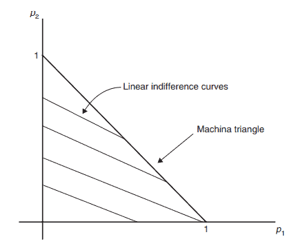
The content of von Neumann-Morgenstern utility theory is easiest to understand in a discrete-state example. Define states $s=1 \ldots S$, each of which is associated with an outcome $x_s$ in a set $X$. Probabilities $p_s$ of the different outcomes then define lotteries. When $S=3$, we can draw probabilities in two dimensions (since $p_3=1-p_1-p_2$ ). We get the so-called Machina triangle (Machina 1982), illustrated in Figure 1.1.

We define a compound lottery as one that determines which primitive lottery we are given. For example, a compound lottery $L$ might give us lottery $L^a$ with probability $\alpha$ and lottery $L^b$ with probability $(1-\alpha)$. Then $L$ has the same probabilities over the outcomes as $\alpha L^a+(1-\alpha) L^b$.

We define a preference ordering $\succeq$ over lotteries. A person is indifferent between lotteries $L^a$ and $L^b, L^a \sim L^b$, if and only if $L^a \succeq L^b$ and $L^b \succeq L^a$.
Next we apply two axioms of choice over lotteries.
Continuity axiom: For all $L^a, L^b, L^c$ s.t. $L^a \succeq L^b \succeq L^c$, there exists a scalar $\alpha \in[0,1]$ s.t.
$$
L^b \sim \alpha L^a+(1-\alpha) L^c .
$$
This axiom says that if three lotteries are (weakly) ranked in order of preference, it is always possible to find a compound lottery that mixes the highest-ranked and lowest-ranked lotteries in such a way that the economic agent is indifferent between this compound lottery and the middle-ranked lottery. The axiom implies the existence of a preference functional defined over lotteries, that is, an ordinal utility function for lotteries that enables us to draw indifference curves on the Machina triangle.

金融代写|波动率模型代写Market Volatility Modelling代考|Risk Aversion

We now assume the existence of a cardinal utility function and ask what it means to say that the agent whose preferences are represented by that utility function is risk averse. We also discuss the quantitative measurement of risk aversion.

To bring out the main ideas as simply as possible, we assume that the argument of the utility function is wealth. This is equivalent to working with a single consumption good in a static two-period model where all wealth is liquidated and consumed in the second period, after uncertainty is resolved. Later in the book we discuss richer models in which consumption takes place in many periods, and also some models with multiple consumption goods.

For simplicity we also work with weak inequalities and weak preference orderings throughout. The extension to strict inequalities and strong preference orderings is straightforward.

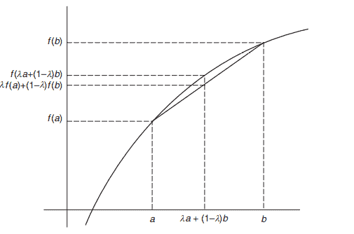
An important mathematical result, Jensen’s Inequality, can be used to link the concept of risk aversion to the concavity of the utility function. We start by defining concavity for a function $f$.

Definition. $f$ is concave if and only if, for all $\lambda \in[0,1]$ and values $a, b$,
$$
\lambda f(a)+(1-\lambda) f(b) \leq f(\lambda a+(1-\lambda) b) .
$$
If $f$ is twice differentiable, then concavity implies that $f^{\prime \prime} \leq 0$. Figure $1.2$ illustrates a concave function.

Note that because the inequality is weak in the above definition, a linear function is concave. Strict concavity uses a strong inequality and excludes linear functions, but we proceed with the weak concept of concavity.
Now consider a random variable $\tilde{z}$. Jensen’s Inequality states that
$$
\mathrm{E} f(\bar{z}) \leq f(\mathrm{E} \bar{z})
$$
for all possible $\tilde{z}$ if and only if $f$ is concave.

金融代写|资产定价代写Asset Pricing代考|FN2190

波动率模型代考

金融代写|波动率模型代写Market Volatility Modelling代考|Expected Utility

标准微观经济学使用有序效用函数表示偏好。序数效用函数 $\Upsilon($.
)tellsyouthatanagentisindifferentbetween $x$ 和 $y$ 如果 $\Upsilon(x)=\Upsilon(y)$ 并且喜欢 $x$ 至 $y$ 如果
$\Upsilon(x)>\Upsilon(y)$. 的任何严格增函数 $\Upsilon($. 将具有相同的属性,因此表示的偏好 $\Upsilon$ (.) arethesameasthose 表示为 $\Theta(\Upsilon()$.) foranystrictlyincreasing $\Theta$. 换句话说,序数效用对于单调递增的变换是不变的。它 定义了无差异曲线,但无法标记曲线以使它们具有有意义的值。
基数效用函数 $\Psi($.$) isinvarianttopositiveaffine(increasinglinear)trans一编队,但不是非线$ 性变换。表达的偏好 $\Psi$ (.)are 与表达的相同 $a+b \Psi($.$) forany b>0$. 换句话说,基数效用没有自然单 位,但如果可以选择单位,基数效用的增长速度是有意义的。
资产定价理论在很大程度上依赖于 von Neumann-Morgenstern 效用理论,该理论认为,对彩票的选择满 足某些公理,意味着对基数效用函数的期望最大化,该函数定义为结果。
von Neumann-Morgenstern 效用理论的内容在一个离散状态的例子中最容易理解。定义状态 $s=1 \ldots S$ ,每一个都与一个结果相关联 $x_s$ 在一组 $X$. 概率 $p_s$ 不同的结果然后定义彩票。什么时候 $S=3$ ,我们可以绘制二维概率 (因为 $p_3=1-p_1-p_2$ ). 我们得到所谓的 Machina 三角形 (Machina 1982),如图 $1.1$ 所示。
我们将复合彩票定义为决定我们获得哪种原始彩票的彩票。例如复合彩票 $L$ 可能会给我们彩票 $L^a$ 有概率 $\alpha$ 和彩票 $L^b$ 有概率 $(1-\alpha)$. 然后 $L$ 对结果的概率与 $\alpha L^a+(1-\alpha) L^b$.
我们定义一个偏好排序 在彩票上。一个人在彩票之间无动于䒾 $L^a$ 和 $L^b, L^a \sim L^b$, 当且仅当 $L^a \succeq L^b$ 和 $L^b \succeq L^a$.
接下来我们对彩票应用两个选择公理。
连续性公理:对于所有 $L^a, L^b, L^c$ 英石 $L^a \succeq L^b \succeq L^c$ ,存在一个标量 $\alpha \in[0,1]$ 英石
$$
L^b \sim \alpha L^a+(1-\alpha) L^c .
$$
这个公理说,如果三种彩票按偏好顺序(弱) 排序,总有可能找到一种复合彩票,它混合了排名最高的彩 票和排名最低的彩票,使得经济主体对这种复合彩票无动于市彩票和中等彩票。该公理意味着存在一个在 彩票上定义的偏好函数,即彩票的序数效用函数使我们能够在 Machina 三角形上绘制无差异曲线。

金融代写|波动率模型代写Market Volatility Modelling代考|Risk Aversion

我们现在假设存在基数效用函数,并询问说其偏好由该效用函数表示的代理人是风险厌恶的是什么意思。 我们还讨论了风险规避的定量测量。
为了尽可能简单地表达主要思想,我们假设效用函数的参数是财富。这相当于在静态双期模型中使用单一 消费品,在不确定性消除后,所有财富都在第二期清算和消费。在本书的后面,我们将讨论更丰富的消费 发生在多个时期的模型,以及一些具有多种消费品的模型。
为简单起见,我们还始终处理弱不等式和弱偏好排序。严格不等式和强偏好排序的扩展很简单。
一个重要的数学结果,詹森不等式,可以用来将风险厌恶的概念与效用函数的凹性联系起来。我们从定义 函数的凹性开始 $f$.
定义。 $f$ 是凹的当且仅当对于所有 $\lambda \in[0,1]$ 和价值观 $a, b$ ,
$$
\lambda f(a)+(1-\lambda) f(b) \leq f(\lambda a+(1-\lambda) b) .
$$
如果 $f$ 是二次可微的,那么凹性意味着 $f^{\prime \prime} \leq 0$. 数字 $1.2$ 说明凹函数。
请注意,由于上述定义中的不等式是弱的,因此线性函数是凹的。严格凹性使用强不等式并排除线性函 数,但我们继续使用凹性的弱概念。
现在考虑一个随机变量 $\tilde{z}$. 詹森不等式指出
$$
\operatorname{E} f(\bar{z}) \leq f(\mathrm{E} \bar{z})
$$
对于所有可能的 $z$ 当且仅当 $f$ 是凹的。

金融代写|波动率模型代写Market Volatility Modelling代考 请认准statistics-lab™

统计代写请认准statistics-lab™. statistics-lab™为您的留学生涯保驾护航。

金融工程代写

金融工程是使用数学技术来解决金融问题。金融工程使用计算机科学、统计学、经济学和应用数学领域的工具和知识来解决当前的金融问题,以及设计新的和创新的金融产品。

非参数统计代写

非参数统计指的是一种统计方法,其中不假设数据来自于由少数参数决定的规定模型;这种模型的例子包括正态分布模型和线性回归模型。

广义线性模型代考

广义线性模型(GLM)归属统计学领域,是一种应用灵活的线性回归模型。该模型允许因变量的偏差分布有除了正态分布之外的其它分布。

术语 广义线性模型(GLM)通常是指给定连续和/或分类预测因素的连续响应变量的常规线性回归模型。它包括多元线性回归,以及方差分析和方差分析(仅含固定效应)。

有限元方法代写

有限元方法(FEM)是一种流行的方法,用于数值解决工程和数学建模中出现的微分方程。典型的问题领域包括结构分析、传热、流体流动、质量运输和电磁势等传统领域。

有限元是一种通用的数值方法,用于解决两个或三个空间变量的偏微分方程(即一些边界值问题)。为了解决一个问题,有限元将一个大系统细分为更小、更简单的部分,称为有限元。这是通过在空间维度上的特定空间离散化来实现的,它是通过构建对象的网格来实现的:用于求解的数值域,它有有限数量的点。边界值问题的有限元方法表述最终导致一个代数方程组。该方法在域上对未知函数进行逼近。[1] 然后将模拟这些有限元的简单方程组合成一个更大的方程系统,以模拟整个问题。然后,有限元通过变化微积分使相关的误差函数最小化来逼近一个解决方案。

tatistics-lab作为专业的留学生服务机构,多年来已为美国、英国、加拿大、澳洲等留学热门地的学生提供专业的学术服务,包括但不限于Essay代写,Assignment代写,Dissertation代写,Report代写,小组作业代写,Proposal代写,Paper代写,Presentation代写,计算机作业代写,论文修改和润色,网课代做,exam代考等等。写作范围涵盖高中,本科,研究生等海外留学全阶段,辐射金融,经济学,会计学,审计学,管理学等全球99%专业科目。写作团队既有专业英语母语作者,也有海外名校硕博留学生,每位写作老师都拥有过硬的语言能力,专业的学科背景和学术写作经验。我们承诺100%原创,100%专业,100%准时,100%满意。

随机分析代写


随机微积分是数学的一个分支,对随机过程进行操作。它允许为随机过程的积分定义一个关于随机过程的一致的积分理论。这个领域是由日本数学家伊藤清在第二次世界大战期间创建并开始的。

时间序列分析代写

随机过程,是依赖于参数的一组随机变量的全体,参数通常是时间。 随机变量是随机现象的数量表现,其时间序列是一组按照时间发生先后顺序进行排列的数据点序列。通常一组时间序列的时间间隔为一恒定值(如1秒,5分钟,12小时,7天,1年),因此时间序列可以作为离散时间数据进行分析处理。研究时间序列数据的意义在于现实中,往往需要研究某个事物其随时间发展变化的规律。这就需要通过研究该事物过去发展的历史记录,以得到其自身发展的规律。

回归分析代写

多元回归分析渐进(Multiple Regression Analysis Asymptotics)属于计量经济学领域,主要是一种数学上的统计分析方法,可以分析复杂情况下各影响因素的数学关系,在自然科学、社会和经济学等多个领域内应用广泛。

MATLAB代写

MATLAB 是一种用于技术计算的高性能语言。它将计算、可视化和编程集成在一个易于使用的环境中,其中问题和解决方案以熟悉的数学符号表示。典型用途包括:数学和计算算法开发建模、仿真和原型制作数据分析、探索和可视化科学和工程图形应用程序开发,包括图形用户界面构建MATLAB 是一个交互式系统,其基本数据元素是一个不需要维度的数组。这使您可以解决许多技术计算问题,尤其是那些具有矩阵和向量公式的问题,而只需用 C 或 Fortran 等标量非交互式语言编写程序所需的时间的一小部分。MATLAB 名称代表矩阵实验室。MATLAB 最初的编写目的是提供对由 LINPACK 和 EISPACK 项目开发的矩阵软件的轻松访问,这两个项目共同代表了矩阵计算软件的最新技术。MATLAB 经过多年的发展,得到了许多用户的投入。在大学环境中,它是数学、工程和科学入门和高级课程的标准教学工具。在工业领域,MATLAB 是高效研究、开发和分析的首选工具。MATLAB 具有一系列称为工具箱的特定于应用程序的解决方案。对于大多数 MATLAB 用户来说非常重要,工具箱允许您学习应用专业技术。工具箱是 MATLAB 函数(M 文件)的综合集合,可扩展 MATLAB 环境以解决特定类别的问题。可用工具箱的领域包括信号处理、控制系统、神经网络、模糊逻辑、小波、仿真等。

R语言代写问卷设计与分析代写
PYTHON代写回归分析与线性模型代写
MATLAB代写方差分析与试验设计代写
STATA代写机器学习/统计学习代写
SPSS代写计量经济学代写
EVIEWS代写时间序列分析代写
EXCEL代写深度学习代写
SQL代写各种数据建模与可视化代写

金融代写|波动率模型代写Market Volatility Modelling代考|COVID19

如果你也在 怎样代写波动率模型Volatility Modelling这个学科遇到相关的难题,请随时右上角联系我们的24/7代写客服。

波动率模型应该能够预测波动率。几乎所有波动率模型的金融用途都需要对未来收益的各个方面进行预测。通常情况下,波动率模型被用来预测收益的绝对幅度,但它也可以用来预测定量,或者,事实上,预测整个密度。

statistics-lab™ 为您的留学生涯保驾护航 在代写波动率模型Volatility Modelling方面已经树立了自己的口碑, 保证靠谱, 高质且原创的统计Statistics代写服务。我们的专家在代写波动率模型Volatility Modelling代写方面经验极为丰富,各种代写波动率模型Volatility Modelling相关的作业也就用不着说。

我们提供的波动率模型Volatility Modelling及其相关学科的代写,服务范围广, 其中包括但不限于:

  • Statistical Inference 统计推断
  • Statistical Computing 统计计算
  • Advanced Probability Theory 高等概率论
  • Advanced Mathematical Statistics 高等数理统计学
  • (Generalized) Linear Models 广义线性模型
  • Statistical Machine Learning 统计机器学习
  • Longitudinal Data Analysis 纵向数据分析
  • Foundations of Data Science 数据科学基础
金融代写|波动率模型代写Market Volatility Modelling代考|COVID19

金融代写|波动率模型代写Market Volatility Modelling代考|Infinitesimal Generators and Associated Martingales

For simplicity we first consider a time-homogeneous diffusion process $\left(X_t\right)$ that solves the stochastic differential equation
$$
d X_t=\mu\left(X_t\right) d t+\sigma\left(X_t\right) d W_t .
$$
Let $g$ be a twice continuously differentiable function of the variable $x$ with bounded derivatives, and define the differential operator $\mathcal{L}$ acting on $g$ according to
$$
\mathcal{L}{\mathcal{G}}(x)-\frac{1}{2} \sigma^2(x) g^{\prime \prime}(x)+\mu(x) g^{\prime}(x) . $$ In terms of $\mathcal{L}$, Itô’s formula (1.16) gives $$ d g\left(X_t\right)=\mathcal{L} g\left(X_t\right) d t+g^{\prime}\left(X_t\right) \sigma\left(X_t\right) d W_t, $$ which shows that $$ M_t=g\left(X_t\right)-\int_0^t \mathcal{L} g\left(X_s\right) d s $$ defines a martingale. Consequently, if $X_0=x$, we obtain $$ \mathbb{E}\left{g\left(X_t\right)\right}=g(x)+\mathbb{E}\left{\int_0^t \mathcal{L} g\left(X_s\right) d s\right} . $$ Under the assumptions made on the coefficients $\mu$ and $\sigma$ and on the function $g$, the Lebesgue dominated convergence theorem is applicable and gives $$ \begin{aligned} \left.\frac{d}{d t} \mathbb{E}\left{g\left(X_t\right)\right}\right|{t=0} & =\lim {t \downarrow 0} \frac{\mathbb{E}\left{g\left(X_t\right)\right}-g(x)}{t} \ & =\lim {t \downarrow 0} \mathbb{E}\left{\frac{1}{t} \int_0^t \mathcal{L} g\left(X_s\right) d s\right}=\mathcal{L} g(x) .
\end{aligned}
$$
The differential operator $\mathcal{L}$ given by (1.61) is called the infinitesimal generator of the Markov process $\left(X_t\right)$.

金融代写|波动率模型代写Market Volatility Modelling代考|Application to the Black-Scholes Partial Differential Equation

In the previous section we assumed the existence, uniqueness, and regularity of the solution of the partial differential equation (1.66) in order to apply Itô’s formula.. A sufficient condition for this is that the coefficients $\mu$ and $\sigma$ are regular enough and that the operator $\mathcal{L}_t$ is uniformly elliptic, meaning (in this one-dimensional situation) that there exists a positive constant $A$ such that
$$
\sigma^2(t, x) \geq A>0 \quad \text { for every } t \geq 0 \text { and } x \in \mathcal{D},
$$
so that the diffusion coefficient $\sigma^2(t, x)$ cannot become too small. Here $\mathcal{D}$ is the domain of the process $\left(X_t\right)$, which may be natural (e.g., $\mathcal{D}={x>0}$ for the geometric Brownian motion) or imposed externally from other modeling considerations.

When $\mu(t, x)=r x$ and $\sigma(t, x)=\sigma x$ in (1.66), we have the Black-Scholes partial differential equation (1.35) on the domain ${x>0}$. The ellipticity condition (1.68) is clearly not satisfied, since the diffusion coefficient $\sigma^2 x^2$ goes to zero as the state variable approaches zero. We get around this difficulty here (and also in more general situations) with the change of variable $P(t, x)=u(t, y=\log x)$, so that equation (1.35) becomes
$$
\frac{\partial u}{\partial t}+\frac{1}{2} \sigma^2 \frac{\partial^2 u}{\partial y^2}+\left(r-\frac{1}{2} \sigma^2\right) \frac{\partial u}{\partial y}-r u=0
$$
to be solved for $0 \leq t \leq T, y \in \mathbb{R}$, and with the final condition $u(T, y)=h\left(e^y\right)$. The operator
$$
\mathcal{L}=\frac{1}{2} \sigma^2 \frac{\partial^2}{\partial y^2}+\left(r-\frac{1}{2} \sigma^2\right) \frac{\partial}{\partial y}
$$
is the infinitesimal generator of the (nonstandard) Brownian motion
$$
Y_t=\left(r-\frac{1}{2} \sigma^2\right) t+\sigma W_t^{\star},
$$
where $\left(W_t^{\star}\right)$ is a standard Brownian motion under $P^{\star}$. We use here the same notation as in the equivalent martingale measure context, but the only important fact is that $W^$ is a standard Brownian motion with respect to the probability used to compute the expectation in the Feynman-Kac formula (1.67). Applying this formula to $Y_t$ yields $$ u(t, y)=\mathbb{E}^\left{e^{-r(T-t)} h\left(e^{y+\left(r-\sigma^2 / 2\right)(T-t)+\sigma\left(W_T^-W_t^\right)} \mid Y_t=y\right}\right.
$$ which is indeed the same as (1.57) by undoing the change of variable $e^y=x$.

金融代写|波动率模型代写Market Volatility Modelling代考|COVID19

波动率模型代考

金融代写|波动率模型代写Market Volatility Modelling代考|Infinitesimal Generators and Associated Martingales

为简单起见,我们首先考虑时间均匀扩散过程 $\left(X_t\right)$ 求解随机微分方程
$$
d X_t=\mu\left(X_t\right) d t+\sigma\left(X_t\right) d W_t .
$$
让 $g$ 是变量的二次连续可微函数 $x$ 有界导数,并定义微分算子 $\mathcal{L}$ 作用于 $g$ 根据
$$
\mathcal{L} \mathcal{G}(x)-\frac{1}{2} \sigma^2(x) g^{\prime \prime}(x)+\mu(x) g^{\prime}(x)
$$
按照 $\mathcal{L}$ , Itô 的公式 (1.16) 给出
$$
d g\left(X_t\right)=\mathcal{L} g\left(X_t\right) d t+g^{\prime}\left(X_t\right) \sigma\left(X_t\right) d W_t
$$
这表明
$$
M_t=g\left(X_t\right)-\int_0^t \mathcal{L} g\left(X_s\right) d s
$$
定义一个鞅。因此,如果 $X_0=x$ ,我们获得
根据对系数所做的假设 $\mu$ 和 $\sigma$ 和功能 $g$, 勒贝格支配的收佥定理适用并给出
微分算子 $\mathcal{L}$ 由 (1.61) 给出的称为马尔可夫过程的无穷小生成器 $\left(X_t\right)$.

金融代写|波动率模型代写Market Volatility Modelling代考|Application to the Black-Scholes Partial Differential Equation

在上一节中,我们假设偏微分方程 (1.66) 的解的存在性、唯一性和正则性,以便应用 Itô 的公式。其充分 条件是系数 $\mu$ 和 $\sigma$ 足够规则,并且操作员 $\mathcal{L}_t$ 是均匀椭圆的,意味着(在这种一维情况下)存在一个正常数 $A$ 这样
$$
\sigma^2(t, x) \geq A>0 \quad \text { for every } t \geq 0 \text { and } x \in \mathcal{D},
$$
使得扩散系数 $\sigma^2(t, x)$ 不能变得太小。这里 $\mathcal{D}$ 是过程的域 $\left(X_t\right)$ ,这可能是自然的(例如, $\mathcal{D}=x>0$ 对 于几何布朗运动) 或从其他建模考虑因素外部施加。
什么时候 $\mu(t, x)=r x$ 和 $\sigma(t, x)=\sigma x$ 在 (1.66) 中,我们在域上有Black-Scholes 偏微分方程 (1.35) $x>0$. 显然不满足椭圆率条件 (1.68),因为扩散系数 $\sigma^2 x^2$ 当状态变量接近零时变为零。我们在这里 (以 及在更一般的情况下) 通过变量的改变来解决这个困难 $P(t, x)=u(t, y=\log x)$, 所以等式 (1.35) 变成
$$
\frac{\partial u}{\partial t}+\frac{1}{2} \sigma^2 \frac{\partial^2 u}{\partial y^2}+\left(r-\frac{1}{2} \sigma^2\right) \frac{\partial u}{\partial y}-r u=0
$$
待解决 $0 \leq t \leq T, y \in \mathbb{R}$, 以及最终条件 $u(T, y)=h\left(e^y\right)$. 运营商
$$
\mathcal{L}=\frac{1}{2} \sigma^2 \frac{\partial^2}{\partial y^2}+\left(r-\frac{1}{2} \sigma^2\right) \frac{\partial}{\partial y}
$$
是 (非标准) 布朗运动的无穷小发生器
$$
Y_t=\left(r-\frac{1}{2} \sigma^2\right) t+\sigma W_t^{\star},
$$
在哪里 $\left(W_t^{\star}\right)$ 是一个标准的布朗运动 $P^{\star}$. 我们在这里使用与等价鞅测度上下文中相同的符号,但唯一重要 的事实是^是关于用于计算 Feynman-Kac 公式 (1.67) 中的期望的概率的标准布朗运动。将此公式应用于 $Y_t$ 产量
通过撤消变量的更改,这确实与 (1.57) 相同 $e^y=x$.

金融代写|波动率模型代写Market Volatility Modelling代考 请认准statistics-lab™

统计代写请认准statistics-lab™. statistics-lab™为您的留学生涯保驾护航。

金融工程代写

金融工程是使用数学技术来解决金融问题。金融工程使用计算机科学、统计学、经济学和应用数学领域的工具和知识来解决当前的金融问题,以及设计新的和创新的金融产品。

非参数统计代写

非参数统计指的是一种统计方法,其中不假设数据来自于由少数参数决定的规定模型;这种模型的例子包括正态分布模型和线性回归模型。

广义线性模型代考

广义线性模型(GLM)归属统计学领域,是一种应用灵活的线性回归模型。该模型允许因变量的偏差分布有除了正态分布之外的其它分布。

术语 广义线性模型(GLM)通常是指给定连续和/或分类预测因素的连续响应变量的常规线性回归模型。它包括多元线性回归,以及方差分析和方差分析(仅含固定效应)。

有限元方法代写

有限元方法(FEM)是一种流行的方法,用于数值解决工程和数学建模中出现的微分方程。典型的问题领域包括结构分析、传热、流体流动、质量运输和电磁势等传统领域。

有限元是一种通用的数值方法,用于解决两个或三个空间变量的偏微分方程(即一些边界值问题)。为了解决一个问题,有限元将一个大系统细分为更小、更简单的部分,称为有限元。这是通过在空间维度上的特定空间离散化来实现的,它是通过构建对象的网格来实现的:用于求解的数值域,它有有限数量的点。边界值问题的有限元方法表述最终导致一个代数方程组。该方法在域上对未知函数进行逼近。[1] 然后将模拟这些有限元的简单方程组合成一个更大的方程系统,以模拟整个问题。然后,有限元通过变化微积分使相关的误差函数最小化来逼近一个解决方案。

tatistics-lab作为专业的留学生服务机构,多年来已为美国、英国、加拿大、澳洲等留学热门地的学生提供专业的学术服务,包括但不限于Essay代写,Assignment代写,Dissertation代写,Report代写,小组作业代写,Proposal代写,Paper代写,Presentation代写,计算机作业代写,论文修改和润色,网课代做,exam代考等等。写作范围涵盖高中,本科,研究生等海外留学全阶段,辐射金融,经济学,会计学,审计学,管理学等全球99%专业科目。写作团队既有专业英语母语作者,也有海外名校硕博留学生,每位写作老师都拥有过硬的语言能力,专业的学科背景和学术写作经验。我们承诺100%原创,100%专业,100%准时,100%满意。

随机分析代写


随机微积分是数学的一个分支,对随机过程进行操作。它允许为随机过程的积分定义一个关于随机过程的一致的积分理论。这个领域是由日本数学家伊藤清在第二次世界大战期间创建并开始的。

时间序列分析代写

随机过程,是依赖于参数的一组随机变量的全体,参数通常是时间。 随机变量是随机现象的数量表现,其时间序列是一组按照时间发生先后顺序进行排列的数据点序列。通常一组时间序列的时间间隔为一恒定值(如1秒,5分钟,12小时,7天,1年),因此时间序列可以作为离散时间数据进行分析处理。研究时间序列数据的意义在于现实中,往往需要研究某个事物其随时间发展变化的规律。这就需要通过研究该事物过去发展的历史记录,以得到其自身发展的规律。

回归分析代写

多元回归分析渐进(Multiple Regression Analysis Asymptotics)属于计量经济学领域,主要是一种数学上的统计分析方法,可以分析复杂情况下各影响因素的数学关系,在自然科学、社会和经济学等多个领域内应用广泛。

MATLAB代写

MATLAB 是一种用于技术计算的高性能语言。它将计算、可视化和编程集成在一个易于使用的环境中,其中问题和解决方案以熟悉的数学符号表示。典型用途包括:数学和计算算法开发建模、仿真和原型制作数据分析、探索和可视化科学和工程图形应用程序开发,包括图形用户界面构建MATLAB 是一个交互式系统,其基本数据元素是一个不需要维度的数组。这使您可以解决许多技术计算问题,尤其是那些具有矩阵和向量公式的问题,而只需用 C 或 Fortran 等标量非交互式语言编写程序所需的时间的一小部分。MATLAB 名称代表矩阵实验室。MATLAB 最初的编写目的是提供对由 LINPACK 和 EISPACK 项目开发的矩阵软件的轻松访问,这两个项目共同代表了矩阵计算软件的最新技术。MATLAB 经过多年的发展,得到了许多用户的投入。在大学环境中,它是数学、工程和科学入门和高级课程的标准教学工具。在工业领域,MATLAB 是高效研究、开发和分析的首选工具。MATLAB 具有一系列称为工具箱的特定于应用程序的解决方案。对于大多数 MATLAB 用户来说非常重要,工具箱允许您学习应用专业技术。工具箱是 MATLAB 函数(M 文件)的综合集合,可扩展 MATLAB 环境以解决特定类别的问题。可用工具箱的领域包括信号处理、控制系统、神经网络、模糊逻辑、小波、仿真等。

R语言代写问卷设计与分析代写
PYTHON代写回归分析与线性模型代写
MATLAB代写方差分析与试验设计代写
STATA代写机器学习/统计学习代写
SPSS代写计量经济学代写
EVIEWS代写时间序列分析代写
EXCEL代写深度学习代写
SQL代写各种数据建模与可视化代写

金融代写|波动率模型代写Market Volatility Modelling代考|FM321

如果你也在 怎样代写波动率模型Volatility Modelling这个学科遇到相关的难题,请随时右上角联系我们的24/7代写客服。

波动率模型应该能够预测波动率。几乎所有波动率模型的金融用途都需要对未来收益的各个方面进行预测。通常情况下,波动率模型被用来预测收益的绝对幅度,但它也可以用来预测定量,或者,事实上,预测整个密度。

statistics-lab™ 为您的留学生涯保驾护航 在代写波动率模型Volatility Modelling方面已经树立了自己的口碑, 保证靠谱, 高质且原创的统计Statistics代写服务。我们的专家在代写波动率模型Volatility Modelling代写方面经验极为丰富,各种代写波动率模型Volatility Modelling相关的作业也就用不着说。

我们提供的波动率模型Volatility Modelling及其相关学科的代写,服务范围广, 其中包括但不限于:

  • Statistical Inference 统计推断
  • Statistical Computing 统计计算
  • Advanced Probability Theory 高等概率论
  • Advanced Mathematical Statistics 高等数理统计学
  • (Generalized) Linear Models 广义线性模型
  • Statistical Machine Learning 统计机器学习
  • Longitudinal Data Analysis 纵向数据分析
  • Foundations of Data Science 数据科学基础
金融代写|波动率模型代写Market Volatility Modelling代考|FM321

金融代写|波动率模型代写Market Volatility Modelling代考|Risk-Neutral Pricing

We mentioned in Section 1.2.1 that, unless $\mu=r$, the expected value under the $s u b$ jective probability $\mathbb{P}$ of the discounted payoff of a derivative (1.23) would lead to an opportunity for arbitrage. This is closely related to the fact that the discounted price $\widetilde{X}_t=e^{-r t} X_t$ is not a martingale since, from (1.18),
$$
d \tilde{X}_t=(\mu-r) \tilde{X}_t d t+\sigma \tilde{X}_t d W_t,
$$
which contains a nonzero drift term if $\mu \neq r$.
The main result we want to build in this section is that there is a unique probability measure $\mathbb{P}^$ equivalent to $\mathbb{P}$ such that, under this probability, (i) the discounted price $\widetilde{X}_t$ is a martingale and (ii) the expected value under $\mathbb{P}^$ of the discounted payoff of a derivative gives its no-arbitrage price. Such a probability measure describing a risk-neutral world is called an equivalent martingale measure.

In order to find a probability measure under which the discounted price $\tilde{X}t$ is a martingale, we rewrite (1.43) in such a way that the drift term is “absorbed” into the martingale term: We set $$ d \widetilde{X}_t=\sigma \widetilde{X}_t\left[d W_t+\left(\frac{\mu-r}{\sigma}\right) d t\right] . $$ $$ \theta=\frac{\mu-r}{\sigma}, $$ called the market price of asset risk, and define $$ W_t^{\star}=W_t+\int_0^t \theta d s=W_t+\theta t, $$ so that $$ d \tilde{X}_t=\sigma \tilde{X}_t d W_t^{\star} . $$ Using the characterization (1.3), it is easy to check that the positive random variable $\xi_T^\theta$ defined by $$ \xi_T^\theta=\exp \left(-\theta W_T-\frac{1}{2} \theta^2 T\right) $$ has an expected value (with respect to $\mathbb{P}$ ) equal to 1 (the Cameron-Martin formula). More generally, it has a conditional expectation with respect to $\mathcal{F}_t$ given by $$ \mathbb{E}\left{\xi_T^\theta \mid \mathcal{F}_t\right}=\exp \left(-\theta W_t-\frac{1}{2} \theta^2 t\right)=\xi_t^\theta \quad \text { for } 0 \leq t \leq T, $$ which defines a martingale denoted by $\left(\xi_t^\theta\right){0 \leq t \leq T}$.
We now introduce the probability measure $\mathbb{P}^{\star}$. It is an equivalent measure to $\mathbb{P}$, meaning that it has the same null sets $\left(\mathbb{P}^*\right.$ and $\mathbb{P}$ agree on which events have zero probability); $\mathbb{P}^{\star}$ has the density $\xi_T^\theta$ with respect to $\mathbb{P}$,
$$
d \mathbb{P}^{\star}=\xi_T^\theta d \mathbb{P} .
$$

金融代写|波动率模型代写Market Volatility Modelling代考|Risk-Neutral Expectations and Partial Differential Equations

In Section 1.4.4 we used the Markov property of the stock price $\left(X_t\right)$ and, in order to compute $X_T$ knowing that $X_t=x$ at time $t \leq T$, we solved the stochastic differential equation (1.2) between $t$ and $T$. This was a particular case of the general situation where $\left(X_t\right)$ is the unique solution of the stochastic differential equation (1.11). We denote by $\left(X_s^{t, x}\right){s \geq t}$ the solution of that equation, starting from $x$ at time $t$ : $$ X_s^{t, x}=x+\int_t^s \mu\left(u, X_u^{t, x}\right) d u+\int_t^s \sigma\left(u, X_u^{t, x}\right) d W_u, $$ and we assume enough regularity in the coefficients $\mu$ and $\sigma$ for $\left(X_s^{t, x}\right)$ to be jointly continuous in the three variables $(t, x, s)$. The flow property for deterministic differential equations can be extended to stochastic differential equations like (1.11); it says that, in order to compute the solution at time $s>t$ starting at time 0 from point $x$, one can use $$ x \longrightarrow X_t^{0, x} \longrightarrow X_s^{1, X_t^{0, x}}=X_s^{0, x} \quad(\mathbb{P} \text {-a.s.). } $$ In other words, one can solve the equation from 0 to $t$, starting from $x$, to obtain $X_t^{0, x}$. Then we solve the equation from $t$ to $s$, starting from $X_t^{0, x}$. This is the same as solving the equation from 0 to $s$, starting from $x$. The Markov property is a consequence and can be stated as follows: $$ \mathbb{E}\left{h\left(X_s\right) \mid \mathcal{F}_1\right}=\left.\mathbb{E}\left{h\left(X_s^{t \cdot x}\right)\right}\right|{x=X_1},
$$
which is what we have used with $s=T$ to derive (1.55). Observe that the discounting factor could be pulled out of the conditional expection since the interest rate is constant (not random). In the time-homogeneous case ( $\mu$ and $\sigma$ independent of time) we further have $$
\mathbb{E}\left{h\left(X_s^{t, X}\right)\right}=\mathbb{E}\left{h\left(X_{s-t}^{0, X}\right)\right},
$$
which could have been used with $s=T$ to derive (1.57) since $W_{T-t}^*$ is $\mathcal{N}(0, T-t)$ distributed.

金融代写|波动率模型代写Market Volatility Modelling代考|FM321

波动率模型代考

金融代写|波动率模型代写Market Volatility Modelling代考|Risk-Neutral Pricing

我们在 1.2.1 节中提到,除非 $\mu=r$ ,下的期望值 $s u b$ 主观概率 $\mathbb{P}$ 衍生品的贴现收益 (1.23) 将带来套利机 会。这与折扣价密切相关 $\widetilde{X}_t=e^{-r t} X_t$ 不是鞅,因为从 (1.18) 开始,
$$
d \tilde{X}_t=(\mu-r) \tilde{X}_t d t+\sigma \tilde{X}_t d W_t,
$$
其中包含一个非零漂移项如果 $\mu \neq r$.
我们要在本节中构建的主要结果是存在唯一的概率度量 $\backslash \mathrm{mathbb}{\mathrm{P}}^{\wedge}$ 相当于 $\mathbb{P}$ 这样,在这个概率下,(i) 折 扣价 $\widetilde{X}_t$ 是一个鞅,并且 (ii) 下的期望值 $\backslash m a t h b b{P} \wedge$ 傠生品的贴现收益给出了它的无套利价格。这种描述 风险中性世界的概率测度称为等价鞅测度。
为了找到折扣价格下的概率测度 $\tilde{X} t$ 是一个鞅,我们重写 (1.43) 使得漂移项被 吸收”到鞅项中:我们设置
$$
\begin{gathered}
d \widetilde{X}_t=\sigma \widetilde{X}_t\left[d W_t+\left(\frac{\mu-r}{\sigma}\right) d t\right] . \
\theta=\frac{\mu-r}{\sigma},
\end{gathered}
$$
称为资产风险的市场价格,定义
$$
W_t^{\star}=W_t+\int_0^t \theta d s=W_t+\theta t
$$
以便
$$
d \tilde{X}_t=\sigma \tilde{X}_t d W_t^{\star} .
$$
使用表征 (1.3),很容易检查正随机变量 $\xi_T^\theta$ 被定义为
$$
\xi_T^\theta=\exp \left(-\theta W_T-\frac{1}{2} \theta^2 T\right)
$$
有一个期望值 (相对于 $\mathbb{P}$ ) 等于 1 (Cameron-Martin 公式)。更一般地,它对 $\mathcal{F}_t$ 由
它定义了一个鞅,表示为 $\left(\xi_t^\theta\right) 0 \leq t \leq T$.
我们现在引入概率度量 $\mathbb{P}^{\star}$. 这是一个等效的措施 $\mathbb{P}$ ,意味着它具有相同的空集 $\left(\mathbb{P}^*\right.$ 和 $\mathbb{P}$ 就哪些事件的概率为 零达成一致); $\mathbb{P}^{\star}$ 有密度 $\xi_T^\theta$ 关于 $\mathbb{P}$ ,
$$
d \mathbb{P}^{\star}=\xi_T^\theta d \mathbb{P} .
$$

金融代写|波动率模型代写Market Volatility Modelling代考|Risk-Neutral Expectations and Partial Differential Equations

在 1.4.4 节中,我们使用了股票价格的马尔可夫属性 $\left(X_t\right)$ 并且,为了计算 $X_T$ 知道 $X_t=x$ 在时间 $t \leq T$ ,我们求解了之间的随机微分方程 (1.2) $t$ 和 $T$. 这是一般情况下的一个特例 $\left(X_t\right)$ 是随机微分方程 (1.11) 的唯一解。我们用 $\left(X_s^{t, x}\right) s \geq t$ 该方程的解,从 $x$ 在时间 $t$ :
$$
X_s^{t, x}=x+\int_t^s \mu\left(u, X_u^{t, x}\right) d u+\int_t^s \sigma\left(u, X_u^{t, x}\right) d W_u,
$$
我们假设系数有足够的规律性 $\mu$ 和 $\sigma$ 为了 $\left(X_s^{t, x}\right)$ 在三个变量中是联合连续的 $(t, x, s)$. 确定性微分方程的 流动性可以扩展到随机微分方程,如 (1.11);它说,为了及时计算解决方案 $s>t$ 从时间 0 开始 $x$ ,可以使 用
$$
x \longrightarrow X_t^{0, x} \longrightarrow X_s^{1, X_t^{0, x}}=X_s^{0, x} \quad(\mathbb{P} \text {-a.s. }) .
$$
从 0 到 $s$ ,从…开始 $x$. 马尔可夫属性是一个结果,可以表述如下:
这是我们用过的 $s=T$ 导出 (1.55)。观察到贴现因子可以从条件预期中提取出来,因为利率是恒定的(不 是随机的)。在时间齐次的情况下 ( $\mu$ 和 $\sigma$ 独立于时间)我们进一步有
Imathbb ${E} \backslash$ eft $\left{h \backslash l\right.$ eft $\left(X_{-} s^{\wedge}{t, X} \backslash\right.$ ight $\left.) \backslash r i g h t\right}=\backslash m a t h b b{E} \backslash l$ eft $\left{h \backslash l\right.$ eft $\left(X_{-}{\right.$st $} \wedge{0, X} \backslash$ ight $) \backslash$ 正确的 $}$ ,
可以与 $s=T$ 导出 (1.57) 因为 $W_{T-t}^*$ 是 $\mathcal{N}(0, T-t)$ 分散式。

金融代写|波动率模型代写Market Volatility Modelling代考 请认准statistics-lab™

统计代写请认准statistics-lab™. statistics-lab™为您的留学生涯保驾护航。

金融工程代写

金融工程是使用数学技术来解决金融问题。金融工程使用计算机科学、统计学、经济学和应用数学领域的工具和知识来解决当前的金融问题,以及设计新的和创新的金融产品。

非参数统计代写

非参数统计指的是一种统计方法,其中不假设数据来自于由少数参数决定的规定模型;这种模型的例子包括正态分布模型和线性回归模型。

广义线性模型代考

广义线性模型(GLM)归属统计学领域,是一种应用灵活的线性回归模型。该模型允许因变量的偏差分布有除了正态分布之外的其它分布。

术语 广义线性模型(GLM)通常是指给定连续和/或分类预测因素的连续响应变量的常规线性回归模型。它包括多元线性回归,以及方差分析和方差分析(仅含固定效应)。

有限元方法代写

有限元方法(FEM)是一种流行的方法,用于数值解决工程和数学建模中出现的微分方程。典型的问题领域包括结构分析、传热、流体流动、质量运输和电磁势等传统领域。

有限元是一种通用的数值方法,用于解决两个或三个空间变量的偏微分方程(即一些边界值问题)。为了解决一个问题,有限元将一个大系统细分为更小、更简单的部分,称为有限元。这是通过在空间维度上的特定空间离散化来实现的,它是通过构建对象的网格来实现的:用于求解的数值域,它有有限数量的点。边界值问题的有限元方法表述最终导致一个代数方程组。该方法在域上对未知函数进行逼近。[1] 然后将模拟这些有限元的简单方程组合成一个更大的方程系统,以模拟整个问题。然后,有限元通过变化微积分使相关的误差函数最小化来逼近一个解决方案。

tatistics-lab作为专业的留学生服务机构,多年来已为美国、英国、加拿大、澳洲等留学热门地的学生提供专业的学术服务,包括但不限于Essay代写,Assignment代写,Dissertation代写,Report代写,小组作业代写,Proposal代写,Paper代写,Presentation代写,计算机作业代写,论文修改和润色,网课代做,exam代考等等。写作范围涵盖高中,本科,研究生等海外留学全阶段,辐射金融,经济学,会计学,审计学,管理学等全球99%专业科目。写作团队既有专业英语母语作者,也有海外名校硕博留学生,每位写作老师都拥有过硬的语言能力,专业的学科背景和学术写作经验。我们承诺100%原创,100%专业,100%准时,100%满意。

随机分析代写


随机微积分是数学的一个分支,对随机过程进行操作。它允许为随机过程的积分定义一个关于随机过程的一致的积分理论。这个领域是由日本数学家伊藤清在第二次世界大战期间创建并开始的。

时间序列分析代写

随机过程,是依赖于参数的一组随机变量的全体,参数通常是时间。 随机变量是随机现象的数量表现,其时间序列是一组按照时间发生先后顺序进行排列的数据点序列。通常一组时间序列的时间间隔为一恒定值(如1秒,5分钟,12小时,7天,1年),因此时间序列可以作为离散时间数据进行分析处理。研究时间序列数据的意义在于现实中,往往需要研究某个事物其随时间发展变化的规律。这就需要通过研究该事物过去发展的历史记录,以得到其自身发展的规律。

回归分析代写

多元回归分析渐进(Multiple Regression Analysis Asymptotics)属于计量经济学领域,主要是一种数学上的统计分析方法,可以分析复杂情况下各影响因素的数学关系,在自然科学、社会和经济学等多个领域内应用广泛。

MATLAB代写

MATLAB 是一种用于技术计算的高性能语言。它将计算、可视化和编程集成在一个易于使用的环境中,其中问题和解决方案以熟悉的数学符号表示。典型用途包括:数学和计算算法开发建模、仿真和原型制作数据分析、探索和可视化科学和工程图形应用程序开发,包括图形用户界面构建MATLAB 是一个交互式系统,其基本数据元素是一个不需要维度的数组。这使您可以解决许多技术计算问题,尤其是那些具有矩阵和向量公式的问题,而只需用 C 或 Fortran 等标量非交互式语言编写程序所需的时间的一小部分。MATLAB 名称代表矩阵实验室。MATLAB 最初的编写目的是提供对由 LINPACK 和 EISPACK 项目开发的矩阵软件的轻松访问,这两个项目共同代表了矩阵计算软件的最新技术。MATLAB 经过多年的发展,得到了许多用户的投入。在大学环境中,它是数学、工程和科学入门和高级课程的标准教学工具。在工业领域,MATLAB 是高效研究、开发和分析的首选工具。MATLAB 具有一系列称为工具箱的特定于应用程序的解决方案。对于大多数 MATLAB 用户来说非常重要,工具箱允许您学习应用专业技术。工具箱是 MATLAB 函数(M 文件)的综合集合,可扩展 MATLAB 环境以解决特定类别的问题。可用工具箱的领域包括信号处理、控制系统、神经网络、模糊逻辑、小波、仿真等。

R语言代写问卷设计与分析代写
PYTHON代写回归分析与线性模型代写
MATLAB代写方差分析与试验设计代写
STATA代写机器学习/统计学习代写
SPSS代写计量经济学代写
EVIEWS代写时间序列分析代写
EXCEL代写深度学习代写
SQL代写各种数据建模与可视化代写

金融代写|波动率模型代写Market Volatility Modelling代考|FE720

如果你也在 怎样代写波动率模型Volatility Modelling这个学科遇到相关的难题,请随时右上角联系我们的24/7代写客服。

波动率模型应该能够预测波动率。几乎所有波动率模型的金融用途都需要对未来收益的各个方面进行预测。通常情况下,波动率模型被用来预测收益的绝对幅度,但它也可以用来预测定量,或者,事实上,预测整个密度。

statistics-lab™ 为您的留学生涯保驾护航 在代写波动率模型Volatility Modelling方面已经树立了自己的口碑, 保证靠谱, 高质且原创的统计Statistics代写服务。我们的专家在代写波动率模型Volatility Modelling代写方面经验极为丰富,各种代写波动率模型Volatility Modelling相关的作业也就用不着说。

我们提供的波动率模型Volatility Modelling及其相关学科的代写,服务范围广, 其中包括但不限于:

  • Statistical Inference 统计推断
  • Statistical Computing 统计计算
  • Advanced Probability Theory 高等概率论
  • Advanced Mathematical Statistics 高等数理统计学
  • (Generalized) Linear Models 广义线性模型
  • Statistical Machine Learning 统计机器学习
  • Longitudinal Data Analysis 纵向数据分析
  • Foundations of Data Science 数据科学基础
金融代写|波动率模型代写Market Volatility Modelling代考|FE720

金融代写|波动率模型代写Market Volatility Modelling代考|Replicating Strategies

The Black-Scholes analysis of a European-style derivative yields an explicit trading strategy in the underlying risky asset and riskless bond whose terminal payoff is equal to the payoff $h\left(X_T\right)$ of the derivative at maturity, no matter what path the stock price takes. Thus, selling the derivative and holding a dynamically adjusted portfolio according to this strategy “covers” an investor against all risk of eventual loss, because a loss incurred at the final time from one part of this portfolio will be exactly compensated by a gain in the other part. This replicating strat$e g y$, as it is known, therefore provides an insurance policy against the risk of being short the derivative. It is called a dynamic hedging strategy since it involves continuous trading, where to hedge means to eliminate risk. The essential step in the Black-Scholes methodology is the construction of this replicating strategy and arguing, based on no arbitrage, that the value of the replicating portfolio at time $t$ is the fair price of the derivative. We develop this argument in the following sections.

We consider a European-style derivative with payoff $h\left(X_T\right)$, a function of the underlying asset price at maturity time $T$. Assume that the stock price $\left(X_t\right)$ follows the geometric Brownian motion model (1.20), a solution of the stochastic differential equation (1.2). A trading strategy is a pair $\left(a_t, b_t\right)$ of adapted processes specifying the number of units held at time $t$ of the underlying asset and the riskless bond, respectively. We suppose that $\mathbb{E}\left{\int_0^T\left(a_t\right)^2 d t\right}$ and $\int_0^T\left|b_t\right| d t$ are finite so that the stochastic integral involving $\left(a_t\right)$ and the usual integral involving $\left(b_t\right)$ are well-defined.

Assuming, as in (1.1), that the price of the bond at time $t$ is $\beta_t=e^{r t}$, the value at time $t$ of this portfolio is $a_t X_t+b_t e^{\prime t}$. It will replicate the derivative at maturity if its value at time $T$ is almost surely equal to the payoff:
$$
a_T X_T+b_T e^{r T}=h\left(X_T\right) .
$$
In addition, this portfolio is to be self-financing, meaning that the variations of its value are due only to the variations of the market – that is, the variations of the stock and bond prices. No further funds are required after the initial investment,yields an instant profit with no exposure to future loss, since the terminal payoff of the trading strategy is equal to the payoff of the derivative.

金融代写|波动率模型代写Market Volatility Modelling代考|Self-Financing Portfolios

As in Section 1.3.1, a portfolio comprises $a_i$ units of stock and $b_t$ in bonds; we denote by $V_t$ its value at time $t$ :
$$
V_t=a_t X_t+b_t e^{r t} .
$$
The self-financing property (1.28), namely $d V_t=a_t d X_t+r b_t e^{r t} d t$, implies that the discounted value of the portfolio, $\widetilde{V}_t=e^{-r t} V_t$, is a martingale under the risk-neutral probability $\mathbb{P}^{\star}$. This important property of self-financing portfolios is cbtained as follows:
$$
\begin{aligned}
d \tilde{V}_t & =-r e^{-r t} V_t d t+e^{-r t} d V_t \
& =-r e^{-r t}\left(a_t X_t+b_t e^{r t}\right) d t-e^{-r t}\left(a_t d X_t+r b_t e^{r t} d t\right) \
& =-r e^{-r t} a_t X_t d t+e^{-r t} a_t d X_t \
& =a_t d\left(e^{-r t} X_t\right) \
& =a_t d \tilde{X}_t \
& =\sigma a_t \widetilde{X}_t d W_t^{\star} \quad(\text { by }(1.46)),
\end{aligned}
$$
which shows that $\left(\tilde{V}_t\right)$ is a martingale under $\mathbb{P}^{\star}$ as a stochastic integral with respect to the Brownian motion $\left(W_t^*\right)$. Indeed, the same computation shows that if a portfolio satisfies $d \tilde{V}_t=a_t d \widetilde{X}_t$ then it is self-financing.

A simple calculation demonstrates the connection between martingales and no arbitrage. Suppose that $\left(a_t, b_t\right)_{0 \leq t \leq T}$ is a self-financing arbitrage strategy; that is,
$$
V_T \geq e^{r T} V_0 \quad(I P \text {-a.s. }),
$$
with
$$
\mathbb{P}\left{V_T>e^{r T} V_0\right}>0,
$$
so that the strategy never makes less than money in the bank and there is some chance of making more. But
$$
\mathbb{E}^\left{V_T\right}=e^{r T} V_0 $$ by the martingale property, so (1.51) and (1.52) cannot hold. This is because $\mathbb{P}$ and $\mathbb{P}^$ are equivalent and so (1.51) and (1.52) also hold with $\mathbb{P}$ replaced by $\mathbb{P}^{\star}$.

金融代写|波动率模型代写Market Volatility Modelling代考|FE720

波动率模型代考

金融代写|波动率模型代写Market Volatility Modelling代考|Replicating Strategies

欧式衍生品的 Black-Scholes 分析得出了一个明确的风险资产和无风险债券的交易策略,其最终收益等于 收益 $h\left(X_T\right)$ 到期时的衍生品,无论股票价格采取何种路径。因此,根据该策略出售衍生品并持有动态调 整的投资组合”覆盖”了投资者最终损失的所有风险,因为在最后时间从该投资组合的一部分中产生的损失 将被另一部分的收益恰好补偿另一部分。这种复制战略egy,众所周知,因此提供了针对做空衍生品风险 的保险单。它被称为动态对冲策略,因为它涉及连续交易,其中对冲意味着消除风险。Black-Scholes 方 法的基本步衼是构建这种复制策略,并在无套利的基础上论证复制投资组合的价值在时间 $t$ 是衍生品的公平 价格。我们在以下各节中展开这一论点。
我们考虑具有收益的欧式衍生品 $h\left(X_T\right)$ ,到期时标的资产价格的函数 $T$. 假设股价 $\left(X_t\right)$ 遵循几何布朗运动 模型 (1.20),随机微分方程 (1.2) 的解。交易策略是一对 $\left(a_t, b_t\right)$ 指定时间持有的单位数量的适应过程 $t$ 分别 的,因此涉及的随机积分 $\left(a_t\right)$ 和通常涉及的积分 $\left(b_t\right)$ 定义明确。
假设,如 (1.1) 中,债券的价格在时间 $t$ 是 $\beta_t=e^{r t}$ ,时间值 $t$ 这个投资组合是 $a_t X_t+b_t e^{\prime t}$. 如果其当时的 价值,它将在到期时复制衍生品 $T$ 几乎肯定等于收益:
$$
a_T X_T+b_T e^{r T}=h\left(X_T\right) .
$$
此外,该投资组合是自筹资金的,这意味看其价值的变化仅取决于市场的变化一一即股票和债券价格的变 化。初始投资后不需要进一步的资金,产生即时利润,没有末来损失的风险,因为交易策略的最终收益等 于衍生品的收益。

金融代写|波动率模型代写Market Volatility Modelling代考|Self-Financing Portfolios

如第 $1.3 .1$ 节所述,投资组合包括 $a_i$ 库存单位和 $b_t$ 债券;我们表示 $V_t$ 它当时的价值 $t$ :
$$
V_t=a_t X_t+b_t e^{r t} .
$$
自筹资金财产 (1.28) ,即 $d V_t=a_t d X_t+r b_t e^{r t} d t$ ,意味着投资组合的贴现值, $\widetilde{V}t=e^{-r t} V_t$ ,是风 险中性概率下的鞅 $\mathbb{P}^{\star}$. 自筹资金组合的这一重要性质如下: $$ d \tilde{V}_t=-r e^{-r t} V_t d t+e^{-r t} d V_t \quad=-r e^{-r t}\left(a_t X_t+b_t e^{r t}\right) d t-e^{-r t}\left(a_t d X_t+r b_t e^{r t} d t\right) $$ 这表明 $\left(\tilde{V}_t\right)$ 是一个鞅 $\mathbb{P}^{\star}$ 作为关于布朗运动的随机积分 $\left(W_t^*\right)$. 事实上,同样的计算表明,如果投资组合满 足 $d \tilde{V}_t=a_t d \widetilde{X}_t$ 然后是自筹资金。 一个简单的计算证明了鞅与无套利之间的联系。假设 $\left(a_t, b_t\right){0 \leq t \leq T}$ 是一种自筹资金的套利策略;那是,
$$
V_T \geq e^{r T} V_0 \quad(I P \text {-a.s. }),
$$

Imathbb ${P} \backslash l$ eft $\left{V_{-} T>e^{\wedge}{r \mathrm{~T}} V_{-} \backslash \backslash\right.$ ight $}>0$,
因此该策略赚取的钱永远不会少于银行里的钱,而且还有赚更多钱的机会。但
Imathbb{E $}^{\wedge} \backslash l$ eft $\left{V_{-} T \backslash r i g h t\right}=e \wedge{r ~ T} \vee_{-} 0$
由鞅性质,所以 (1.51) 和 (1.52) 不能成立。这是因为 $\mathbb{P}$ 和 \mathbb ${P} \wedge$ 是等价的,所以 (1.51) 和 (1.52) 也 成立 $\mathbb{P}$ 取而代之 $\mathbb{P}^{\star}$.

金融代写|波动率模型代写Market Volatility Modelling代考 请认准statistics-lab™

统计代写请认准statistics-lab™. statistics-lab™为您的留学生涯保驾护航。

金融工程代写

金融工程是使用数学技术来解决金融问题。金融工程使用计算机科学、统计学、经济学和应用数学领域的工具和知识来解决当前的金融问题,以及设计新的和创新的金融产品。

非参数统计代写

非参数统计指的是一种统计方法,其中不假设数据来自于由少数参数决定的规定模型;这种模型的例子包括正态分布模型和线性回归模型。

广义线性模型代考

广义线性模型(GLM)归属统计学领域,是一种应用灵活的线性回归模型。该模型允许因变量的偏差分布有除了正态分布之外的其它分布。

术语 广义线性模型(GLM)通常是指给定连续和/或分类预测因素的连续响应变量的常规线性回归模型。它包括多元线性回归,以及方差分析和方差分析(仅含固定效应)。

有限元方法代写

有限元方法(FEM)是一种流行的方法,用于数值解决工程和数学建模中出现的微分方程。典型的问题领域包括结构分析、传热、流体流动、质量运输和电磁势等传统领域。

有限元是一种通用的数值方法,用于解决两个或三个空间变量的偏微分方程(即一些边界值问题)。为了解决一个问题,有限元将一个大系统细分为更小、更简单的部分,称为有限元。这是通过在空间维度上的特定空间离散化来实现的,它是通过构建对象的网格来实现的:用于求解的数值域,它有有限数量的点。边界值问题的有限元方法表述最终导致一个代数方程组。该方法在域上对未知函数进行逼近。[1] 然后将模拟这些有限元的简单方程组合成一个更大的方程系统,以模拟整个问题。然后,有限元通过变化微积分使相关的误差函数最小化来逼近一个解决方案。

tatistics-lab作为专业的留学生服务机构,多年来已为美国、英国、加拿大、澳洲等留学热门地的学生提供专业的学术服务,包括但不限于Essay代写,Assignment代写,Dissertation代写,Report代写,小组作业代写,Proposal代写,Paper代写,Presentation代写,计算机作业代写,论文修改和润色,网课代做,exam代考等等。写作范围涵盖高中,本科,研究生等海外留学全阶段,辐射金融,经济学,会计学,审计学,管理学等全球99%专业科目。写作团队既有专业英语母语作者,也有海外名校硕博留学生,每位写作老师都拥有过硬的语言能力,专业的学科背景和学术写作经验。我们承诺100%原创,100%专业,100%准时,100%满意。

随机分析代写


随机微积分是数学的一个分支,对随机过程进行操作。它允许为随机过程的积分定义一个关于随机过程的一致的积分理论。这个领域是由日本数学家伊藤清在第二次世界大战期间创建并开始的。

时间序列分析代写

随机过程,是依赖于参数的一组随机变量的全体,参数通常是时间。 随机变量是随机现象的数量表现,其时间序列是一组按照时间发生先后顺序进行排列的数据点序列。通常一组时间序列的时间间隔为一恒定值(如1秒,5分钟,12小时,7天,1年),因此时间序列可以作为离散时间数据进行分析处理。研究时间序列数据的意义在于现实中,往往需要研究某个事物其随时间发展变化的规律。这就需要通过研究该事物过去发展的历史记录,以得到其自身发展的规律。

回归分析代写

多元回归分析渐进(Multiple Regression Analysis Asymptotics)属于计量经济学领域,主要是一种数学上的统计分析方法,可以分析复杂情况下各影响因素的数学关系,在自然科学、社会和经济学等多个领域内应用广泛。

MATLAB代写

MATLAB 是一种用于技术计算的高性能语言。它将计算、可视化和编程集成在一个易于使用的环境中,其中问题和解决方案以熟悉的数学符号表示。典型用途包括:数学和计算算法开发建模、仿真和原型制作数据分析、探索和可视化科学和工程图形应用程序开发,包括图形用户界面构建MATLAB 是一个交互式系统,其基本数据元素是一个不需要维度的数组。这使您可以解决许多技术计算问题,尤其是那些具有矩阵和向量公式的问题,而只需用 C 或 Fortran 等标量非交互式语言编写程序所需的时间的一小部分。MATLAB 名称代表矩阵实验室。MATLAB 最初的编写目的是提供对由 LINPACK 和 EISPACK 项目开发的矩阵软件的轻松访问,这两个项目共同代表了矩阵计算软件的最新技术。MATLAB 经过多年的发展,得到了许多用户的投入。在大学环境中,它是数学、工程和科学入门和高级课程的标准教学工具。在工业领域,MATLAB 是高效研究、开发和分析的首选工具。MATLAB 具有一系列称为工具箱的特定于应用程序的解决方案。对于大多数 MATLAB 用户来说非常重要,工具箱允许您学习应用专业技术。工具箱是 MATLAB 函数(M 文件)的综合集合,可扩展 MATLAB 环境以解决特定类别的问题。可用工具箱的领域包括信号处理、控制系统、神经网络、模糊逻辑、小波、仿真等。

R语言代写问卷设计与分析代写
PYTHON代写回归分析与线性模型代写
MATLAB代写方差分析与试验设计代写
STATA代写机器学习/统计学习代写
SPSS代写计量经济学代写
EVIEWS代写时间序列分析代写
EXCEL代写深度学习代写
SQL代写各种数据建模与可视化代写

金融代写|市场微观结构与算法交易代写Market Microstructure and Algorithmic Trading代考|FIN602

如果你也在 怎样代写市场微观结构与算法交易Market Microstructure and Algorithmic Trading这个学科遇到相关的难题,请随时右上角联系我们的24/7代写客服。

市场微观结构分析了特定的交易机制如何影响价格形成过程。微观结构涉及市场结构和设计,价格形成和价格发现,交易和时间成本,信息和披露,以及做市商和投资者行为等问题。

statistics-lab™ 为您的留学生涯保驾护航 在代写市场微观结构与算法交易Market Microstructure and Algorithmic Trading方面已经树立了自己的口碑, 保证靠谱, 高质且原创的统计Statistics代写服务。我们的专家在代写市场微观结构与算法交易Market Microstructure and Algorithmic Trading代写方面经验极为丰富,各种代写市场微观结构与算法交易Market Microstructure and Algorithmic Trading相关的作业也就用不着说。

我们提供的市场微观结构与算法交易Market Microstructure and Algorithmic Trading及其相关学科的代写,服务范围广, 其中包括但不限于:

  • Statistical Inference 统计推断
  • Statistical Computing 统计计算
  • Advanced Probability Theory 高等概率论
  • Advanced Mathematical Statistics 高等数理统计学
  • (Generalized) Linear Models 广义线性模型
  • Statistical Machine Learning 统计机器学习
  • Longitudinal Data Analysis 纵向数据分析
  • Foundations of Data Science 数据科学基础
金融代写|市场微观结构与算法交易代写Market Microstructure and Algorithmic Trading代考|FIN602

金融代写|市场微观结构与算法交易代写Market Microstructure and Algorithmic Trading代考|Market microstructure

Despite the beauty and simplicity of MPT and CAPM, the theory they rely on, i.e. the Efficient Market Theory (EMT) is too reductionistic and idealistic when compared with real market conditions. Therefore, MPT and CAPM must be handled with care since they both can lead to wrong conclusions.

Let us study each one of the hypotheses of the EMT, the framework in which MPT and CAPM were developed.

  1. Existence of a single market price.
    According to the theory, market prices reflect the fundamental value of assets. However, the very notion of price is very ambiguous. Indeed, in any market we have several prices coexisting simultaneously: ask price, bid price, mid-point, last traded price, average price, etc. Moreover, this single-price assumption ignores the price formation process, depends on the subtleties of each market and explains why do we have different prices at different markets and.
  2. Information is complete and perfect.
    According to EMT, economic information is complete, perfect and everyone has access to it. Therefore, if investors are rational they will all have the same expectations on the future behavior of assets. In practice this is not true because there exists and asymmetry of information. Indeed, not only information has a price (e.g. real-time access via Bloomberg or Reuters) but also markets have different degrees of transparency (e.g. dark pools).
  3. All investors are equal.
    If all investors were rational and share the same information then they would all have the same expectations on the future value of assets, and in consequence they would all have the same behavior. However, since there is a huge heterogeneity of investors it is not realistic at all to consider that all investors are equal, as the EMT does. Indeed, each single investor has a personal strategy (long-only, long-short, hedging, speculation, arbitrage), a time horizon (ranging from several years to milliseconds) and an asset preference (equities, foreign exchange, interest rates, credit, derivatives, venture capital).

金融代写|市场微观结构与算法交易代写Market Microstructure and Algorithmic Trading代考|Market orders

A Market order is an instruction to trade a given quantity at the best price possible. Market orders demand liquidity because their focus is on completing the order. Therefore, the main risk is the uncertainty of the ultimate execution price: if the volume at the current market price is not enough then the market order jumps to the next level of the order book; this process goes on until the order is fully executed.

A Limit order is an instruction to trade a given quantity at a specified price or better. A buy limit order must execute at or below this limit price, whereas a sell order must execute at or above it.
A Market-to-limit order is an hybrid instruction constituted by a market order with an implicit price limit. When the order arrives it behaves as a market order, seeking liquidity at the best price available, which we call the entry price. As soon as the order starts to execute, it becomes a limit-order with limit price equals to the entry price. Unlike a traditional market order, a market-to-limit order does not sweep the order book. If there is insufficient liquidity available at the best price, the order will convert into a standing limit order for the residual amount.

A Stop order is an extension of the market-to-limit order with a limit price further away from the last execution price: the trading is activated or stopped when a certain threshold price is reached. There are three important examples of stop orders. Stop-loss orders are designed to protect a potential gain: for long (resp. short) positions the execution is stopped if prices go above (resp. below) the threshold. Contingent or if-touched orders remain hidden until the threshold is reached, in which case they become active; hence, they are the mirror orders of stop-loss. Stop limit orders have two thresholds, one that activates the order and the other one that deactivates it; hence, they are a hybrid built with one stop-loss and one contingent order.
An Iceberg order is an order with a small part visible in the order book and a significantly larger hidden volume. These orders slice the total amount to be exchanged into several tranches. The first tranche constitutes the visible part, and as soon as it is completely executed the next tranche becomes visible. The interest of iceberg orders is that they provide an automated slicing program for orders of big size. However, the hidden tranches lose time priority in the order book; they only have price priority.

A Peg order is an instruction with a dynamic limit price. The price is automatically adjusted according to the evolution the spread: for long (resp. short) positions they always hit the best bid (resp. ask) price. In consequence, peg orders are always first in price priority and second in time priority. There are also peg orders with stop-limits, which follow the best price until it reaches the deactivating threshold.

金融代写|市场微观结构与算法交易代写Market Microstructure and Algorithmic Trading代考|FIN602

市场微观结构与算法交易代考

金融代写|市场微观结构与算法交易代写Market Microstructure and Algorithmic Trading代考|Market microstructure

尽管 MPT 和 CAPM 既美观又简单,但与实际市场条件相比,它们所依赖的理论,即有效市场理论 (EMT) 过于简化和理想化。因此,必须谨慎处理 MPT 和 CAPM,因为它们都可能导致错误的结论。

让我们研究一下 EMT 的每一个假设,EMT 是 MPT 和 CAPM 开发的框架。

  1. 存在单一市场价格。
    根据该理论,市场价格反映了资产的基本价值。然而,价格的概念非常模糊。事实上,在任何市场中,我们都有几个价格同时存在:卖价、买价、中间价、最后交易价、平均价等。而且,这种单一价格假设忽略了价格形成过程,取决于每个价格的微妙之处市场并解释为什么我们在不同的市场有不同的价格。
  2. 信息完整、完善。
    根据 EMT,经济信息是完整的、完美的,每个人都可以访问它。因此,如果投资者是理性的,他们对资产的未来行为都会有相同的预期。实际上,这是不正确的,因为存在信息不对称。事实上,不仅信息有价格(例如通过彭博社或路透社的实时访问),而且市场也有不同程度的透明度(例如暗池)。
  3. 所有投资者都是平等的。
    如果所有投资者都是理性的并且共享相同的信息,那么他们对资产的未来价值都会有相同的预期,因此他们都会有相同的行为。然而,由于投资者存在巨大的异质性,因此像 EMT 那样认为所有投资者都是平等的根本不现实。事实上,每个投资者都有自己的个人策略(多头、多头、空头、对冲、投机、套利)、时间范围(从几年到几毫秒不等)和资产偏好(股票、外汇、利率、信贷、衍生品、风险投资)。

金融代写|市场微观结构与算法交易代写Market Microstructure and Algorithmic Trading代考|Market orders

市价单是指以尽可能最好的价格交易给定数量的指令。市场订单需要流动性,因为它们的重点是完成订单。因此,主要的风险是最终执行价格的不确定性:如果当前市场价格的成交量不够,则市价订单跳转到订单簿的下一级;这个过程一直持续到订单完全执行。

限价订单是指以指定价格或更好的价格交易给定数量的指令。买入限价单必须以或低于此限价执行,而卖出订单必须以或高于此限价执行。
市价转限价单是由隐含价格限制的市价单构成的混合指令。当订单到达时,它表现为市场订单,以可用的最佳价格寻求流动性,我们称之为入场价。一旦订单开始执行,它就变成限价订单,限价等于入场价。与传统的市价订单不同,市价到限价订单不会清除订单簿。如果最佳价格的可用流动性不足,则该订单将转换为剩余金额的常设限价订单。

止损订单是市价到限价订单的扩展,其限价距离最后执行价格更远:当达到某个阈值价格时,交易被激活或停止。止损订单有三个重要的例子。止损订单旨在保护潜在收益:对于多头(或空头)头寸,如果价格高于(或低于)阈值,则执行将停止。在达到阈值之前,或有订单或触及订单将保持隐藏状态,在这种情况下它们会变为活动订单;因此,它们是止损的镜像订单。止损限价订单有两个阈值,一个激活订单,另一个关闭订单;因此,它们是一种由一个止损单和一个或有订单组成的混合体。
冰山订单是订单簿中有一小部分可见且隐藏量明显更大的订单。这些订单将要交换的总金额分成几部分。第一部分构成可见部分,一旦完全执行,下一部分就会变得可见。冰山订单的好处在于它们为大订单提供自动切片程序。然而,隐藏的部分在订单簿中失去了时间优先权;他们只有价格优先。

挂钩订单是一种具有动态限价的指令。价格根据价差的演变自动调整:对于多头(或空头)头寸,他们总是达到最佳买价(或卖价)。因此,挂钩订单总是价格优先,时间优先。也有带有止损限价的挂钩订单,它们会跟随最佳价格,直到达到停用阈值。

金融代写|量化风险管理代写Quantitative Risk Management代考 请认准statistics-lab™

统计代写请认准statistics-lab™. statistics-lab™为您的留学生涯保驾护航。

金融工程代写

金融工程是使用数学技术来解决金融问题。金融工程使用计算机科学、统计学、经济学和应用数学领域的工具和知识来解决当前的金融问题,以及设计新的和创新的金融产品。

非参数统计代写

非参数统计指的是一种统计方法,其中不假设数据来自于由少数参数决定的规定模型;这种模型的例子包括正态分布模型和线性回归模型。

广义线性模型代考

广义线性模型(GLM)归属统计学领域,是一种应用灵活的线性回归模型。该模型允许因变量的偏差分布有除了正态分布之外的其它分布。

术语 广义线性模型(GLM)通常是指给定连续和/或分类预测因素的连续响应变量的常规线性回归模型。它包括多元线性回归,以及方差分析和方差分析(仅含固定效应)。

有限元方法代写

有限元方法(FEM)是一种流行的方法,用于数值解决工程和数学建模中出现的微分方程。典型的问题领域包括结构分析、传热、流体流动、质量运输和电磁势等传统领域。

有限元是一种通用的数值方法,用于解决两个或三个空间变量的偏微分方程(即一些边界值问题)。为了解决一个问题,有限元将一个大系统细分为更小、更简单的部分,称为有限元。这是通过在空间维度上的特定空间离散化来实现的,它是通过构建对象的网格来实现的:用于求解的数值域,它有有限数量的点。边界值问题的有限元方法表述最终导致一个代数方程组。该方法在域上对未知函数进行逼近。[1] 然后将模拟这些有限元的简单方程组合成一个更大的方程系统,以模拟整个问题。然后,有限元通过变化微积分使相关的误差函数最小化来逼近一个解决方案。

tatistics-lab作为专业的留学生服务机构,多年来已为美国、英国、加拿大、澳洲等留学热门地的学生提供专业的学术服务,包括但不限于Essay代写,Assignment代写,Dissertation代写,Report代写,小组作业代写,Proposal代写,Paper代写,Presentation代写,计算机作业代写,论文修改和润色,网课代做,exam代考等等。写作范围涵盖高中,本科,研究生等海外留学全阶段,辐射金融,经济学,会计学,审计学,管理学等全球99%专业科目。写作团队既有专业英语母语作者,也有海外名校硕博留学生,每位写作老师都拥有过硬的语言能力,专业的学科背景和学术写作经验。我们承诺100%原创,100%专业,100%准时,100%满意。

随机分析代写


随机微积分是数学的一个分支,对随机过程进行操作。它允许为随机过程的积分定义一个关于随机过程的一致的积分理论。这个领域是由日本数学家伊藤清在第二次世界大战期间创建并开始的。

时间序列分析代写

随机过程,是依赖于参数的一组随机变量的全体,参数通常是时间。 随机变量是随机现象的数量表现,其时间序列是一组按照时间发生先后顺序进行排列的数据点序列。通常一组时间序列的时间间隔为一恒定值(如1秒,5分钟,12小时,7天,1年),因此时间序列可以作为离散时间数据进行分析处理。研究时间序列数据的意义在于现实中,往往需要研究某个事物其随时间发展变化的规律。这就需要通过研究该事物过去发展的历史记录,以得到其自身发展的规律。

回归分析代写

多元回归分析渐进(Multiple Regression Analysis Asymptotics)属于计量经济学领域,主要是一种数学上的统计分析方法,可以分析复杂情况下各影响因素的数学关系,在自然科学、社会和经济学等多个领域内应用广泛。

MATLAB代写

MATLAB 是一种用于技术计算的高性能语言。它将计算、可视化和编程集成在一个易于使用的环境中,其中问题和解决方案以熟悉的数学符号表示。典型用途包括:数学和计算算法开发建模、仿真和原型制作数据分析、探索和可视化科学和工程图形应用程序开发,包括图形用户界面构建MATLAB 是一个交互式系统,其基本数据元素是一个不需要维度的数组。这使您可以解决许多技术计算问题,尤其是那些具有矩阵和向量公式的问题,而只需用 C 或 Fortran 等标量非交互式语言编写程序所需的时间的一小部分。MATLAB 名称代表矩阵实验室。MATLAB 最初的编写目的是提供对由 LINPACK 和 EISPACK 项目开发的矩阵软件的轻松访问,这两个项目共同代表了矩阵计算软件的最新技术。MATLAB 经过多年的发展,得到了许多用户的投入。在大学环境中,它是数学、工程和科学入门和高级课程的标准教学工具。在工业领域,MATLAB 是高效研究、开发和分析的首选工具。MATLAB 具有一系列称为工具箱的特定于应用程序的解决方案。对于大多数 MATLAB 用户来说非常重要,工具箱允许您学习应用专业技术。工具箱是 MATLAB 函数(M 文件)的综合集合,可扩展 MATLAB 环境以解决特定类别的问题。可用工具箱的领域包括信号处理、控制系统、神经网络、模糊逻辑、小波、仿真等。

R语言代写问卷设计与分析代写
PYTHON代写回归分析与线性模型代写
MATLAB代写方差分析与试验设计代写
STATA代写机器学习/统计学习代写
SPSS代写计量经济学代写
EVIEWS代写时间序列分析代写
EXCEL代写深度学习代写
SQL代写各种数据建模与可视化代写

金融代写|市场微观结构与算法交易代写Market Microstructure and Algorithmic Trading代考|QF302

如果你也在 怎样代写市场微观结构与算法交易Market Microstructure and Algorithmic Trading这个学科遇到相关的难题,请随时右上角联系我们的24/7代写客服。

市场微观结构分析了特定的交易机制如何影响价格形成过程。微观结构涉及市场结构和设计,价格形成和价格发现,交易和时间成本,信息和披露,以及做市商和投资者行为等问题。

statistics-lab™ 为您的留学生涯保驾护航 在代写市场微观结构与算法交易Market Microstructure and Algorithmic Trading方面已经树立了自己的口碑, 保证靠谱, 高质且原创的统计Statistics代写服务。我们的专家在代写市场微观结构与算法交易Market Microstructure and Algorithmic Trading代写方面经验极为丰富,各种代写市场微观结构与算法交易Market Microstructure and Algorithmic Trading相关的作业也就用不着说。

我们提供的市场微观结构与算法交易Market Microstructure and Algorithmic Trading及其相关学科的代写,服务范围广, 其中包括但不限于:

  • Statistical Inference 统计推断
  • Statistical Computing 统计计算
  • Advanced Probability Theory 高等概率论
  • Advanced Mathematical Statistics 高等数理统计学
  • (Generalized) Linear Models 广义线性模型
  • Statistical Machine Learning 统计机器学习
  • Longitudinal Data Analysis 纵向数据分析
  • Foundations of Data Science 数据科学基础
金融代写|市场微观结构与算法交易代写Market Microstructure and Algorithmic Trading代考|QF302

金融代写|市场微观结构与算法交易代写Market Microstructure and Algorithmic Trading代考|Optimal trading curve

When it comes to intraday trading strategies we have the following dilemma, also known the trader’s dilemma: If we trade slow then prices will move away from their current quote, i.e. we are facing a market risk; however, if we trade fast then our order will drive quotes away from the current one, i.e. we will have a great market impact (see Figure 1.4).

Recall that in MPT we optimize the joint effect of two oppossite forces: minimizing the risk of the portfolio and maximizing the (expected) return. Following the idea of the efficient frontier, it seems natural to build up a optimization program that minimizes simultaneously both market risk and market impact.

Suppose we need to sell a certain amount of asset $S$ during the day. We split the trading order in exactly $N$ small sub-orders of size $\nu_n, n=1, \ldots, N$. The goal is to find the right trading proportions
$$
\nu_i \geq 0, \quad i=1, \ldots, N ; \quad \sum_{n=1}^N \nu_n=1,
$$
that minimize the expected loss due to market risk and market impact.
As we will see in later chapters, the set of minimizers constitute a curve, the optimal trading curve. For a given risk level (variance), the trading strategy $P$ on the optimal trading curve is the one that minimizes the expected market costs, i.e. the joint effects of market risk and market impact (see Figure 1.3).

金融代写|市场微观结构与算法交易代写Market Microstructure and Algorithmic Trading代考|The scope of this m´emoire

The goal of this mémoire is to describe thoroughly the construction of the optimal trading curve $\left(x_0, \ldots, x_N\right)$ for different market models and portfolio strategies.

In Chapter 2 we will study the market microstructure. We will see how the hypotheses of MPT and CAPM, i.e. the Efficient Market Theory, are all violated in real markets. We will focus in particular on the effect of transaction costs and market impact. We will also review the benchmarks used for monitoring trades.

Roughly speaking, a trading strategy is algorithmic if it is stripped of human decisions (and emotions). In Chapter 3 we will describe what is algorithmic trading. We will survey the basic strategies in algorithmic trading, which are the bricks with which almost any systematic trading strategy can be constructed. We will also show evidence that favors algorithmic over human trading.

In Chapter 4 we will construct the optimal trading curve $\left(x_0, \ldots, x_N\right)$ under normality assumptions, i.e. where the asset follows a Brownian motion. This chapter will be based on the article of Almgren and Chriss [1] for single assets and on the work of Lehalle [14] for multi-asset

In Chapter 5 we will construct again the optimal trading curve $\left(x_0, \ldots, x_N\right)$, but following Lehalle [14] we will consider that the portfolio has mean-reverting dynamics. We will solve analytically and numerical a simplified case of a mean-reverting portfolio using the shooting method, which is a numerical technique used in differential equations. The novelty of our approach is the alternative optimization program we use: we will construct the optimal trading curve using 1-dimensional algorithm regardless of the total number of trades $N$. Being more advantageous than the classical approaches based on functional optimization in $\mathbb{R}^N$, this approach could be of interest for systematic brokers and traders.

Chapter 6 is the final chapter. We will make some remarks on the portfolio models we have presented and mention some possible extensions. We will also review several alternative models for time series that could be used to describe markets more accurately. Finally, we will comment on the pros and cons of automated (algorithmic-based) trading with respect to discretionary (human-based) trading.

金融代写|市场微观结构与算法交易代写Market Microstructure and Algorithmic Trading代考|QF302

市场微观结构与算法交易代考

金融代写|市场微观结构与算法交易代写Market Microstructure and Algorithmic Trading代考|Optimal trading curve

当谈到日内交易策略时,我们面临以下困境,也称为交易者困境: 如果我们交易缓慢,那么价格将偏离当 前报价,即我们面临市场风险;然而,如果我们快速交易,那么我们的订单将使报价远离当前订单,即我 们将产生巨大的市场影响(见图 1.4)。
回想一下,在 MPT 中,我们优化了两种相反力量的联合效应:最小化投资组合的风险和最大化(预期) 回报。按照有效边界的想法,建立一个同时最小化市场风险和市场影响的优化程序似乎很自然。
假设我们需要出售一定数量的资产 $S$ 白天。我们将交易订单完全拆分 $N$ 尺寸小的子订单 $\nu_n, n=1, \ldots, N$. 目标是找到合适的交易比例
$$
\nu_i \geq 0, \quad i=1, \ldots, N ; \quad \sum_{n=1}^N \nu_n=1,
$$
最大限度地减少因市场风险和市场影响造成的预期损失。
正如我们将在后面的章节中看到的那样,一组最小值构成了一条曲线,即最优交易曲线。对于给定的风险 水平 (方差),交易策略 $P$ 在最优交易曲线上的是最小化预期市场成本的曲线,即市场风险和市场影响的 联合效应 (见图 1.3)。

金融代写|市场微观结构与算法交易代写Market Microstructure and Algorithmic Trading代考|The scope of this m´emoire

这篇回忆录的目的是彻底描述最佳交易曲线的构造(X0,…,X否)针对不同的市场模型和投资组合策略。

在第 2 章中,我们将研究市场微观结构。我们将看到 MPT 和 CAPM 的假设,即有效市场理论,在真实市场中是如何被违反的。我们将特别关注交易成本和市场影响的影响。我们还将审查用于监控交易的基准。

粗略地说,如果一个交易策略被剥夺了人为决定(和情绪),它就是算法。在第 3 章中,我们将描述什么是算法交易。我们将调查算法交易中的基本策略,这些策略是几乎可以构建任何系统交易策略的砖块。我们还将展示支持算法交易优于人工交易的证据。

在第 4 章中我们将构建最优交易曲线(X0,…,X否)在正常假设下,即资产遵循布朗运动。本章将基于 Almgren 和 Chriss [1] 针对单一资产的文章以及 Lehalle [14] 针对多资产的工作

在第 5 章我们将再次构建最优交易曲线(X0,…,X否),但根据 Lehalle [14],我们将考虑投资组合具有均值回归动态。我们将使用射击法分析和数值求解一个均值回归投资组合的简化案例,射击法是微分方程中使用的一种数值技术。我们方法的新颖之处在于我们使用的替代优化程序:我们将使用一维算法构建最优交易曲线,而不管交易总数否. 比基于功能优化的经典方法更具优势R否, 这种方法可能会引起系统经纪人和交易者的兴趣。

第六章是最终章。我们将对我们提出的投资组合模型做出一些评论,并提及一些可能的扩展。我们还将审查几种可用于更准确地描述市场的时间序列替代模型。最后,我们将评论自动(基于算法的)交易相对于全权委托(基于人工的)交易的优缺点。

金融代写|量化风险管理代写Quantitative Risk Management代考 请认准statistics-lab™

统计代写请认准statistics-lab™. statistics-lab™为您的留学生涯保驾护航。

金融工程代写

金融工程是使用数学技术来解决金融问题。金融工程使用计算机科学、统计学、经济学和应用数学领域的工具和知识来解决当前的金融问题,以及设计新的和创新的金融产品。

非参数统计代写

非参数统计指的是一种统计方法,其中不假设数据来自于由少数参数决定的规定模型;这种模型的例子包括正态分布模型和线性回归模型。

广义线性模型代考

广义线性模型(GLM)归属统计学领域,是一种应用灵活的线性回归模型。该模型允许因变量的偏差分布有除了正态分布之外的其它分布。

术语 广义线性模型(GLM)通常是指给定连续和/或分类预测因素的连续响应变量的常规线性回归模型。它包括多元线性回归,以及方差分析和方差分析(仅含固定效应)。

有限元方法代写

有限元方法(FEM)是一种流行的方法,用于数值解决工程和数学建模中出现的微分方程。典型的问题领域包括结构分析、传热、流体流动、质量运输和电磁势等传统领域。

有限元是一种通用的数值方法,用于解决两个或三个空间变量的偏微分方程(即一些边界值问题)。为了解决一个问题,有限元将一个大系统细分为更小、更简单的部分,称为有限元。这是通过在空间维度上的特定空间离散化来实现的,它是通过构建对象的网格来实现的:用于求解的数值域,它有有限数量的点。边界值问题的有限元方法表述最终导致一个代数方程组。该方法在域上对未知函数进行逼近。[1] 然后将模拟这些有限元的简单方程组合成一个更大的方程系统,以模拟整个问题。然后,有限元通过变化微积分使相关的误差函数最小化来逼近一个解决方案。

tatistics-lab作为专业的留学生服务机构,多年来已为美国、英国、加拿大、澳洲等留学热门地的学生提供专业的学术服务,包括但不限于Essay代写,Assignment代写,Dissertation代写,Report代写,小组作业代写,Proposal代写,Paper代写,Presentation代写,计算机作业代写,论文修改和润色,网课代做,exam代考等等。写作范围涵盖高中,本科,研究生等海外留学全阶段,辐射金融,经济学,会计学,审计学,管理学等全球99%专业科目。写作团队既有专业英语母语作者,也有海外名校硕博留学生,每位写作老师都拥有过硬的语言能力,专业的学科背景和学术写作经验。我们承诺100%原创,100%专业,100%准时,100%满意。

随机分析代写


随机微积分是数学的一个分支,对随机过程进行操作。它允许为随机过程的积分定义一个关于随机过程的一致的积分理论。这个领域是由日本数学家伊藤清在第二次世界大战期间创建并开始的。

时间序列分析代写

随机过程,是依赖于参数的一组随机变量的全体,参数通常是时间。 随机变量是随机现象的数量表现,其时间序列是一组按照时间发生先后顺序进行排列的数据点序列。通常一组时间序列的时间间隔为一恒定值(如1秒,5分钟,12小时,7天,1年),因此时间序列可以作为离散时间数据进行分析处理。研究时间序列数据的意义在于现实中,往往需要研究某个事物其随时间发展变化的规律。这就需要通过研究该事物过去发展的历史记录,以得到其自身发展的规律。

回归分析代写

多元回归分析渐进(Multiple Regression Analysis Asymptotics)属于计量经济学领域,主要是一种数学上的统计分析方法,可以分析复杂情况下各影响因素的数学关系,在自然科学、社会和经济学等多个领域内应用广泛。

MATLAB代写

MATLAB 是一种用于技术计算的高性能语言。它将计算、可视化和编程集成在一个易于使用的环境中,其中问题和解决方案以熟悉的数学符号表示。典型用途包括:数学和计算算法开发建模、仿真和原型制作数据分析、探索和可视化科学和工程图形应用程序开发,包括图形用户界面构建MATLAB 是一个交互式系统,其基本数据元素是一个不需要维度的数组。这使您可以解决许多技术计算问题,尤其是那些具有矩阵和向量公式的问题,而只需用 C 或 Fortran 等标量非交互式语言编写程序所需的时间的一小部分。MATLAB 名称代表矩阵实验室。MATLAB 最初的编写目的是提供对由 LINPACK 和 EISPACK 项目开发的矩阵软件的轻松访问,这两个项目共同代表了矩阵计算软件的最新技术。MATLAB 经过多年的发展,得到了许多用户的投入。在大学环境中,它是数学、工程和科学入门和高级课程的标准教学工具。在工业领域,MATLAB 是高效研究、开发和分析的首选工具。MATLAB 具有一系列称为工具箱的特定于应用程序的解决方案。对于大多数 MATLAB 用户来说非常重要,工具箱允许您学习应用专业技术。工具箱是 MATLAB 函数(M 文件)的综合集合,可扩展 MATLAB 环境以解决特定类别的问题。可用工具箱的领域包括信号处理、控制系统、神经网络、模糊逻辑、小波、仿真等。

R语言代写问卷设计与分析代写
PYTHON代写回归分析与线性模型代写
MATLAB代写方差分析与试验设计代写
STATA代写机器学习/统计学习代写
SPSS代写计量经济学代写
EVIEWS代写时间序列分析代写
EXCEL代写深度学习代写
SQL代写各种数据建模与可视化代写

金融代写|市场微观结构与算法交易代写Market Microstructure and Algorithmic Trading代考|FE570

如果你也在 怎样代写市场微观结构与算法交易Market Microstructure and Algorithmic Trading这个学科遇到相关的难题,请随时右上角联系我们的24/7代写客服。

市场微观结构分析了特定的交易机制如何影响价格形成过程。微观结构涉及市场结构和设计,价格形成和价格发现,交易和时间成本,信息和披露,以及做市商和投资者行为等问题。

statistics-lab™ 为您的留学生涯保驾护航 在代写市场微观结构与算法交易Market Microstructure and Algorithmic Trading方面已经树立了自己的口碑, 保证靠谱, 高质且原创的统计Statistics代写服务。我们的专家在代写市场微观结构与算法交易Market Microstructure and Algorithmic Trading代写方面经验极为丰富,各种代写市场微观结构与算法交易Market Microstructure and Algorithmic Trading相关的作业也就用不着说。

我们提供的市场微观结构与算法交易Market Microstructure and Algorithmic Trading及其相关学科的代写,服务范围广, 其中包括但不限于:

  • Statistical Inference 统计推断
  • Statistical Computing 统计计算
  • Advanced Probability Theory 高等概率论
  • Advanced Mathematical Statistics 高等数理统计学
  • (Generalized) Linear Models 广义线性模型
  • Statistical Machine Learning 统计机器学习
  • Longitudinal Data Analysis 纵向数据分析
  • Foundations of Data Science 数据科学基础
金融代写|市场微观结构与算法交易代写Market Microstructure and Algorithmic Trading代考|FE570

金融代写|市场微观结构与算法交易代写Market Microstructure and Algorithmic Trading代考|Modern Portfolio Theory (MPT) and efficient frontier

MPT (or Markowitz Portfolio) was developed by Markowitz in 1952. The idea behind MPT is simple yet insightful. Imagine a market with two assets $A$ and $B$, in which we invest today $(t=0)$ and at time $t=1$ we recover our initial investment plus the profits of the period. Assume that the probability distributions of $A$ and $B$ are known, i.e. their means $r_A, r_B$ and variances $\sigma_A, \sigma_B$ are information available to everybody.
Suppose $r_A>r_B$ and $\sigma_A>\sigma_B$. Then we have two natural choices:

  • Maximize profits regardless of the risk (i.e. variance). In this case we choose asset $A$.
  • Minimize risk regardless of profit. In this case we choose $B$.
    Now suppose that the correlation $\rho$ between both assets is negative and that short-selling is not allowed. Then there exists an investment strategy $\omega \in(0,1)$ such that the corresponding portfolio
    $$
    P=\omega A+(1-\omega) B
    $$
    has minimal variance, i.e. $\sigma_P<\sigma_B$. Portfolio $P$ is called the minimal variance portfolio (see Figure 1.1).

In general, if the market consists on $N$ assets $A_1, \ldots, A_N$, there is an investment strategy
$$
\omega_i \geq 0, \quad i=1, \ldots, N ; \quad \sum_{i=1}^N \omega_i=1
$$ such that the portfolio
$$
P=\sum_{i=1}^N \omega_i A_i
$$
has minimal variance, i.e.
$$
\sigma_P \leq \min \left{\sigma_i: i=1, \ldots, N\right} .
$$
Moreover, if at least one of the correlations is negative then inequality (1.1) is strict.
Now suppose we want to minimize the variance of our portfolio $P$ for a given target return $r$. Then the optimization program is to minimize $\sigma_P$ under the constraints
$$
\omega_i \geq 0, \quad i=1, \ldots, N ; \quad \sum_{i=1}^N \omega_i=1 ; \quad \sum_{i=1}^N \omega_i r_i=r .
$$
Analogously, for a given risk level $\sigma$ we can maximize the portfolio return $r_p$ under the constraints
$$
\omega_i \geq 0, \quad i=1, \ldots, N ; \quad \sum_{i=1}^N \omega_i=1 ; \quad \sigma_P=\sigma .
$$

金融代写|市场微观结构与算法交易代写Market Microstructure and Algorithmic Trading代考|Capital Asset Pricing Model (CAPM) and betas

MPT is a great idea that relies on the calculation of the variance-covariance matrix. However, when the number of assets grows it becomes very hard to calculate. Indeed, For $N$ assets, since the $N \times N$ variance-covariance matrix is symmetric it has $N(N+1) / 2$ degrees of freedom (See Table 1.1).

In order to overcome this difficulty, we could try to calculate first a market portfolio, which includes all available assets, and then compare this market portfolio with each and every one of the single assets. If we proceed this way then the number of degrees of freedom is $2(N+1)$ : $N+1$ volatilities and $N+1$ correlations. This is far more manageable than the $N(N+1) / 2$ degrees of freedom in MPT.

This is the idea behind CAPM, which was developed by Sharpe, a PhD student of Markowitz, in 1964. According to CAPM, the return of an asset $i$ is
$$
r^i=r^f+\beta_{i M}\left(r^M-r^f\right)+\varepsilon_i, \quad \beta_{i M}=\frac{\operatorname{cov}\left(r^i, r^M\right)}{\operatorname{var}\left(r^M\right)},
$$
where $r^i$ is the return of asset $i, r^f$ the return of the risk-free asset (e.g. Treasure bonds) and $r^M$ the market return. $\beta_{i M}$ is the marginal contribution of asset $i$ to market risk, also known as the systematic risk or market risk, whereas $\varepsilon_i$ is the idiosyncratic risk. The idiosincratic risk can be eliminated via diversification, whereas the systematic risk is inherent of the market and cannot be diversified away.

Now let us study the relative returns with respect to the risk-free asset. Taking expectations in (1.2) it follows that that the expected return of asset $i$ over the risk-less rate $r_f$ is
$$
E\left(r^i-r^f\right)=\beta_{i M} E\left(r^M-r^f\right) .
$$
As we can see from (1.2), the beta of asset $i$ (i.e. its systematic risk $\beta_{i M}$ ) acts as an amplifier of the expected market returns (see Figure 1.3).

金融代写|市场微观结构与算法交易代写Market Microstructure and Algorithmic Trading代考|FE570

市场微观结构与算法交易代考

金融代写|市场微观结构与算法交易代写Market Microstructure and Algorithmic Trading代考|Modern Portfolio Theory (MPT) and efficient frontier

MPT (或 Markowitz 投资组合) 由 Markowitz 于 1952 年开发。MPT 背后的理念简单而富有洞察力。想 象一个有两种资产的市场 $A$ 和 $B$ ,我们今天投资的 $(t=0)$ 并且在时间 $t=1$ 我们收回了我们的初始投资加 上当期的利润。假设概率分布 $A$ 和 $B$ 是已知的,即他们的手段 $r_A, r_B$ 和方差 $\sigma_A, \sigma_B$ 是每个人都可以获得 的信息。
认为 $r_A>r_B$ 和 $\sigma_A>\sigma_B$. 那么我们有两个自然的选择:

  • 不考虑风险(即方差),实现利润最大化。在这种情况下,我们选择资产 $A$.
  • 无论利润如何,都将风险降至最低。在这种情况下我们选择 $B$. 现在假设相关性 $\rho$ 两种资产之间为负,不允许卖空。那么存在一个投资策略 $\omega \in(0,1)$ 这样相应的投 资组合
    $$
    P=\omega A+(1-\omega) B
    $$
    方差最小,即 $\sigma_P<\sigma_B$. 文件夹 $P$ 称为最小方差投资组合(见图 1.1)。
    一般来说,如果市场由 $N$ 资产 $A_1, \ldots, A_N$ ,有一个投资策略
    $$
    \omega_i \geq 0, \quad i=1, \ldots, N ; \quad \sum_{i=1}^N \omega_i=1
    $$
    这样投资组合
    $$
    P=\sum_{i=1}^N \omega_i A_i
    $$
    方差最小,即
    此外,如果至少一个相关性为负,则不等式 (1.1) 是严格的。
    现在假设我们想要最小化投资组合的方差 $P$ 对于给定的目标回报 $r$. 那么优化方案就是最小化 $\sigma_P$ 约束之下
    $$
    \omega_i \geq 0, \quad i=1, \ldots, N ; \quad \sum_{i=1}^N \omega_i=1 ; \quad \sum_{i=1}^N \omega_i r_i=r .
    $$
    类似地,对于给定的风险水平 $\sigma$ 我们可以最大化投资组合回报 $r_p$ 约束之下
    $$
    \omega_i \geq 0, \quad i=1, \ldots, N ; \quad \sum_{i=1}^N \omega_i=1 ; \quad \sigma_P=\sigma
    $$

金融代写|市场微观结构与算法交易代写Market Microstructure and Algorithmic Trading代考|Capital Asset Pricing Model (CAPM) and betas

MPT 是一个很棒的想法,它依赖于方差-协方差矩阵的计算。然而,当资产数量增加时,计算变得非常困 难。的确,为了 $N$ 资产,自 $N \times N$ 方差-协方差矩阵是对称的它有 $N(N+1) / 2$ 自由度(见表 1.1)。
为了克服这个困难,我们可以尝试先计算一个市场组合,其中包括所有可用资产,然后将这个市场组合与 每一个单一资产进行比较。如果我们以这种方式进行,那么自由度的数量是 $2(N+1): N+1$ 波动率和 $N+1$ 相关性。这比 $N(N+1) / 2 \mathrm{MPT}$ 中的自由度。
这就是 CAPM 背后的想法,它是由 Markowitz 的博士生 Sharpe 在 1964 年开发的。根据 CAPM,资产的 回报率 $i$ 是
$$
r^i=r^f+\beta_{i M}\left(r^M-r^f\right)+\varepsilon_i, \quad \beta_{i M}=\frac{\operatorname{cov}\left(r^i, r^M\right)}{\operatorname{var}\left(r^M\right)},
$$
在哪里 $r^i$ 是资产回报 $i, r^f$ 无风险资产 (例如国债) 的回报和 $r^M$ 市场回报。 $\beta_{i M}$ 是资产的边际贡献 $i$ 市场风 险,也称为系统风险或市场风险,而 $\varepsilon_i$ 是特殊风险。异质性风险可以通过分散化消除,而系统性风险是市 场固有的,无法通过分散化消除。
现在让我们研究无风险资产的相对回报。考虑 (1.2) 中的期望,可以得出资产的期望收益 $i$ 超过无风险利率 $r_f$ 是
$$
E\left(r^i-r^f\right)=\beta_{i M} E\left(r^M-r^f\right) .
$$
从式 (1.2) 可以看出,资产的贝塔 $i$ (即其系统性风险 $\beta_{i M}$ ) 充当预期市场回报的放大器(见图 1.3)。

金融代写|量化风险管理代写Quantitative Risk Management代考 请认准statistics-lab™

统计代写请认准statistics-lab™. statistics-lab™为您的留学生涯保驾护航。

金融工程代写

金融工程是使用数学技术来解决金融问题。金融工程使用计算机科学、统计学、经济学和应用数学领域的工具和知识来解决当前的金融问题,以及设计新的和创新的金融产品。

非参数统计代写

非参数统计指的是一种统计方法,其中不假设数据来自于由少数参数决定的规定模型;这种模型的例子包括正态分布模型和线性回归模型。

广义线性模型代考

广义线性模型(GLM)归属统计学领域,是一种应用灵活的线性回归模型。该模型允许因变量的偏差分布有除了正态分布之外的其它分布。

术语 广义线性模型(GLM)通常是指给定连续和/或分类预测因素的连续响应变量的常规线性回归模型。它包括多元线性回归,以及方差分析和方差分析(仅含固定效应)。

有限元方法代写

有限元方法(FEM)是一种流行的方法,用于数值解决工程和数学建模中出现的微分方程。典型的问题领域包括结构分析、传热、流体流动、质量运输和电磁势等传统领域。

有限元是一种通用的数值方法,用于解决两个或三个空间变量的偏微分方程(即一些边界值问题)。为了解决一个问题,有限元将一个大系统细分为更小、更简单的部分,称为有限元。这是通过在空间维度上的特定空间离散化来实现的,它是通过构建对象的网格来实现的:用于求解的数值域,它有有限数量的点。边界值问题的有限元方法表述最终导致一个代数方程组。该方法在域上对未知函数进行逼近。[1] 然后将模拟这些有限元的简单方程组合成一个更大的方程系统,以模拟整个问题。然后,有限元通过变化微积分使相关的误差函数最小化来逼近一个解决方案。

tatistics-lab作为专业的留学生服务机构,多年来已为美国、英国、加拿大、澳洲等留学热门地的学生提供专业的学术服务,包括但不限于Essay代写,Assignment代写,Dissertation代写,Report代写,小组作业代写,Proposal代写,Paper代写,Presentation代写,计算机作业代写,论文修改和润色,网课代做,exam代考等等。写作范围涵盖高中,本科,研究生等海外留学全阶段,辐射金融,经济学,会计学,审计学,管理学等全球99%专业科目。写作团队既有专业英语母语作者,也有海外名校硕博留学生,每位写作老师都拥有过硬的语言能力,专业的学科背景和学术写作经验。我们承诺100%原创,100%专业,100%准时,100%满意。

随机分析代写


随机微积分是数学的一个分支,对随机过程进行操作。它允许为随机过程的积分定义一个关于随机过程的一致的积分理论。这个领域是由日本数学家伊藤清在第二次世界大战期间创建并开始的。

时间序列分析代写

随机过程,是依赖于参数的一组随机变量的全体,参数通常是时间。 随机变量是随机现象的数量表现,其时间序列是一组按照时间发生先后顺序进行排列的数据点序列。通常一组时间序列的时间间隔为一恒定值(如1秒,5分钟,12小时,7天,1年),因此时间序列可以作为离散时间数据进行分析处理。研究时间序列数据的意义在于现实中,往往需要研究某个事物其随时间发展变化的规律。这就需要通过研究该事物过去发展的历史记录,以得到其自身发展的规律。

回归分析代写

多元回归分析渐进(Multiple Regression Analysis Asymptotics)属于计量经济学领域,主要是一种数学上的统计分析方法,可以分析复杂情况下各影响因素的数学关系,在自然科学、社会和经济学等多个领域内应用广泛。

MATLAB代写

MATLAB 是一种用于技术计算的高性能语言。它将计算、可视化和编程集成在一个易于使用的环境中,其中问题和解决方案以熟悉的数学符号表示。典型用途包括:数学和计算算法开发建模、仿真和原型制作数据分析、探索和可视化科学和工程图形应用程序开发,包括图形用户界面构建MATLAB 是一个交互式系统,其基本数据元素是一个不需要维度的数组。这使您可以解决许多技术计算问题,尤其是那些具有矩阵和向量公式的问题,而只需用 C 或 Fortran 等标量非交互式语言编写程序所需的时间的一小部分。MATLAB 名称代表矩阵实验室。MATLAB 最初的编写目的是提供对由 LINPACK 和 EISPACK 项目开发的矩阵软件的轻松访问,这两个项目共同代表了矩阵计算软件的最新技术。MATLAB 经过多年的发展,得到了许多用户的投入。在大学环境中,它是数学、工程和科学入门和高级课程的标准教学工具。在工业领域,MATLAB 是高效研究、开发和分析的首选工具。MATLAB 具有一系列称为工具箱的特定于应用程序的解决方案。对于大多数 MATLAB 用户来说非常重要,工具箱允许您学习应用专业技术。工具箱是 MATLAB 函数(M 文件)的综合集合,可扩展 MATLAB 环境以解决特定类别的问题。可用工具箱的领域包括信号处理、控制系统、神经网络、模糊逻辑、小波、仿真等。

R语言代写问卷设计与分析代写
PYTHON代写回归分析与线性模型代写
MATLAB代写方差分析与试验设计代写
STATA代写机器学习/统计学习代写
SPSS代写计量经济学代写
EVIEWS代写时间序列分析代写
EXCEL代写深度学习代写
SQL代写各种数据建模与可视化代写

金融代写|量化风险管理代写Quantitative Risk Management代考|PROJMGNT1002

如果你也在 怎样代写量化风险管理Quantitative Risk Management这个学科遇到相关的难题,请随时右上角联系我们的24/7代写客服。

项目管理中的定量风险管理是将风险对项目的影响转换为数字的过程。这种数字信息经常被用来确定项目的成本和时间应急措施。

statistics-lab™ 为您的留学生涯保驾护航 在代写量化风险管理Quantitative Risk Management方面已经树立了自己的口碑, 保证靠谱, 高质且原创的统计Statistics代写服务。我们的专家在代写量化风险管理Quantitative Risk Management代写方面经验极为丰富,各种代写量化风险管理Quantitative Risk Management相关的作业也就用不着说。

我们提供的量化风险管理Quantitative Risk Management及其相关学科的代写,服务范围广, 其中包括但不限于:

  • Statistical Inference 统计推断
  • Statistical Computing 统计计算
  • Advanced Probability Theory 高等概率论
  • Advanced Mathematical Statistics 高等数理统计学
  • (Generalized) Linear Models 广义线性模型
  • Statistical Machine Learning 统计机器学习
  • Longitudinal Data Analysis 纵向数据分析
  • Foundations of Data Science 数据科学基础
金融代写|量化风险管理代写Quantitative Risk Management代考|PROJMGNT1002

金融代写|量化风险管理代写Quantitative Risk Management代考|Risks faced by a financial firm

Decrease in the value of the investments on the asset side of the balance sheet (e.g. losses from securities trading or credit risk).

  • Maturity mismatch (large parts of the assets are relatively illiquid (longterm) whereas large parts of the liabilities are rather short-term obligations. This can lead to a default of a solvent bank or a bank run).
  • The prime risk for an insurer is insolvency (risk that claims of policy holders cannot be met). On the asset side, risks are similar to those of a bank. On the liability side, the main risk is that reserves are insufficient
  • to cover future claim payments. Note that the liabilities of a life insurer are of a long-term nature and subject to multiple categories of risk (e.g. interest rate risk, inflation risk and longevity risk).
  • So risk is found on both sides of the balance sheet and thus RM should not focus on the asset side alone.
  • There are different notions of capital. One distinguishes:
    Equity capital $\quad-$ Value of assets – debt;
  • Measures the firm’s value to its shareholders;
  • Can be split into shareholder capital (initial capital invested in the firm) and retained earnings (accumulated earnings not paid to shareholders).
    Regulatory capital – Capital required according to regulatory rules;
  • For European insurance firms: Minimum (MCR) and solvency capital requirements (SCR);
  • A regulatory framework also specifies the capital quality. One distinguishes Tier 1 capital (i.e. shareholder capital + retained earnings; can act in full as buffer) and Tier 2 capital (includes other positions on the balance sheet).
  • Capital required to control the probability of becoming insolvent (typically over one year);
  • Internal assessment of risk capital;
  • Aims at a holistic view (assets and liabilities) and works with fair values of balance sheet items.

金融代写|量化风险管理代写Quantitative Risk Management代考|Modelling value and value change

We set up a general mathematical model for (changes in) value caused by financial risks. To this end we work on a probability space $(\Omega, \mathcal{F}, \mathbb{P})$ and consider a risk or loss as a random variable $X: \Omega \rightarrow \mathbb{R}($ or: $L$ ).

  • Consider a portfolio of assets and possibly liabilities. The value of the portfolio at time $t$ (today) is denoted by $V_t$ (a random variable; assumed to be known at $t$; its $d f$ is typically not trivial to determine!).
  • We consider a given time horizon $\Delta t$ and assume:
    1) the portfolio composition remains fixed over $\Delta t$;
    2) there are no intermediate payments during $\Delta t$
    $\Rightarrow$ Fine for small $\Delta t$ but unlikely to hold for large $\Delta t$.
  • The change in value of the portfolio is given by
    $$
    \Delta V_{t+1}=V_{t+1}-V_t
    $$
    and we define the (random) loss by the sign-adjusted value change
    $$
    L_{t+1}=-\Delta V_{t+1}
    $$
    (as QRM is mainly concerned with losses).

1) The distribution of $L_{t+1}$ is called loss distribution.
2) Practitioners often consider the profit-and-loss $(P \& L)$ distribution which is the distribution of $-L_{t+1}=\Delta V_{t+1}$.
3) For longer time intervals, $\Delta V_{t+1}=V_{t+1} /(1+r)-V_t$ ( $r=$ risk-free interest rate) would be more appropriate, but we will mostly neglect this issue.

  • $V_t$ is typically modelled as a function $f$ of time $t$ and a $d$-dimensional random vector $\boldsymbol{Z}=\left(Z_{t, 1}, \ldots, Z_{t, d}\right)$ of risk factors, that is,
    $$
    V_t=f\left(t, \boldsymbol{Z}t\right) \quad \text { (mapping of risks) } $$ for some measurable $f: \mathbb{R}{+} \times \mathbb{R}^d \rightarrow \mathbb{R}$. The choice of $f$ and $\boldsymbol{Z}_t$ is problem-specific (typically known, but possibly difficult to evaluate).
  • It is often convenient to work with the risk-factor changes
    $$
    \boldsymbol{X}{t+1}=\boldsymbol{Z}{t+1}-\boldsymbol{Z}t . $$ We can rewrite $L{t+1}$ in terms of $\boldsymbol{X}{t+1}$ via $$ \begin{aligned} L{t+1} & =-\left(V_{t+1}-V_t\right)=-\left(f\left(t+1, \boldsymbol{Z}{t+1}\right)-f\left(t, \boldsymbol{Z}_t\right)\right) \ & =-\left(f\left(t+1, \boldsymbol{Z}_t+\boldsymbol{X}{t+1}\right)-f\left(t, \boldsymbol{Z}t\right)\right) \end{aligned} $$ We see that the loss $d f$ is determined by the loss df of $X{t+1}$. We will thus also write $L_{t+1}=L\left(\boldsymbol{X}_{t+1}\right)$, where $L(\boldsymbol{x})=-\left(f\left(t+1, \boldsymbol{Z}_t+\boldsymbol{x}\right)-f\left(t, \boldsymbol{Z}_t\right)\right)$ is known as loss operator.
金融代写|量化风险管理代写Quantitative Risk Management代考|PROJMGNT1002

量化风险管理代考

金融代写|量化风险管理代写Quantitative Risk Management代考|Risks faced by a financial firm

资产负债表资产端的投资价值下降(例如,证券交易损失或信用风险)。

  • 期限错配(大部分资产流动性相对较差(长期),而大部分负债是相当短期的债务。这可能导致有偿付能力的银行违约或银行挤兑)。
  • 保险公司面临的主要风险是资不抵债(无法满足保单持有人索赔的风险)。在资产方面,风险类似于银行的风险。负债端,主要风险是准备金不足
  • 以支付未来的理赔费用。请注意,人寿保险公司的负债具有长期性质,并受到多种风险的影响(例如利率风险、通胀风险和长寿风险)。
  • 因此,资产负债表的两边都存在风险,因此 RM 不应只关注资产方面。
  • 有不同的资本概念。一区分:
    股权资本−资产价值——债务;
  • 衡量公司对其股东的价值;
  • 可以分为股东资本(投资于公司的初始资本)和留存收益(未支付给股东的累计收益)。
    监管资本——监管规定要求的资本;
  • 对于欧洲保险公司:最低 (MCR) 和偿付能力资本要求 (SCR);
  • 监管框架还规定了资本质量。一种区分一级资本(即股东资本+留存收益;可以完全作为缓冲)和二级资本(包括资产负债表上的其他头寸)。
  • 控制破产可能性所需的资本(通常超过一年);
  • 风险资本内部评估;
  • 以整体观点(资产和负债)为目标,并处理资产负债表项目的公允价值。

金融代写|量化风险管理代写Quantitative Risk Management代考|Modelling value and value change

我们为金融风险引起的价值 (变化) 建立了一个通用的数学模型。为此,我们在概率空间上工作 $(\Omega, \mathcal{F}, \mathbb{P})$ 并将风险或损失视为随机变量 $X: \Omega \rightarrow \mathbb{R}($ 或者: $L$ ).

  • 考虑一个资产组合,可能还有负债。投资组合当时的价值 $t$ (今天) 表示为 $V_t$ (一个随机变量; 假设 在 $t ;$ 它的 $d f$ 确定起来通常不是微不足道的))。
  • 我们考虑给定的时间范围 $\Delta t$ 并假设:
    1) 投资组合构成在 $\Delta t$;
    2)期间没有中间付款 $\Delta t$
    $\Rightarrow$ 适合小的 $\Delta t$ 但不太可能长期持有 $\Delta t$.
  • 投资组合价值的变化由下式给出
    $$
    \Delta V_{t+1}=V_{t+1}-V_t
    $$
    我们通过符号调整后的值变化来定义 (随机) 损失
    $$
    L_{t+1}=-\Delta V_{t+1}
    $$
    (因为 $\mathrm{QRM}$ 主要关注损失) 。
    1) 分布 $L_{t+1}$ 称为损失分布。
    2) 从业者往往考虑盈亏 $(P \& L)$ 分布这是分布 $-L_{t+1}=\Delta V_{t+1}$.
    3) 对于更长的时间间隔, $\Delta V_{t+1}=V_{t+1} /(1+r)-V_t(r=$ 无风险利率) 会更合适,但我们大多会 忽略这个问题。
  • $V_t$ 通常被建模为一个函数 $f$ 时间的 $t$ 和一个 $d$ 维随机向量 $\boldsymbol{Z}=\left(Z_{t, 1}, \ldots, Z_{t, d}\right)$ 的风险因素,即
    $$
    V_t=f(t, \boldsymbol{Z} t) \quad \text { (mapping of risks) }
    $$
    对于一些可测量的 $f: \mathbb{R}+\times \mathbb{R}^d \rightarrow \mathbb{R}$. 的选择 $f$ 和 $Z_t$ 是特定于问题的(通常是已知的,但可能难 以评估)。
  • 处理风险因素变化通常很方便
    $$
    \boldsymbol{X} t+1=\boldsymbol{Z} t+1-\boldsymbol{Z} t .
    $$
    我们可以重写 $L t+1$ 按照 $\boldsymbol{X} t+1$ 通过
    $$
    L t+1=-\left(V_{t+1}-V_t\right)=-\left(f(t+1, \boldsymbol{Z} t+1)-f\left(t, \boldsymbol{Z}t\right)\right) \quad=-\left(f \left(t+1, \boldsymbol{Z}_t+\boldsymbol{X} t\right.\right. $$ 我们看到损失 $d f$ 由损失 df 决定 $X t+1$. 因此我们也将写 $L{t+1}=L\left(\boldsymbol{X}_{t+1}\right)$ ,在哪里$L(\boldsymbol{x})=-\left(f\left(t+1, \boldsymbol{Z}_t+\boldsymbol{x}\right)-f\left(t, \boldsymbol{Z}_t\right)\right)$ 被称为损失算子。
金融代写|量化风险管理代写Quantitative Risk Management代考 请认准statistics-lab™

统计代写请认准statistics-lab™. statistics-lab™为您的留学生涯保驾护航。

金融工程代写

金融工程是使用数学技术来解决金融问题。金融工程使用计算机科学、统计学、经济学和应用数学领域的工具和知识来解决当前的金融问题,以及设计新的和创新的金融产品。

非参数统计代写

非参数统计指的是一种统计方法,其中不假设数据来自于由少数参数决定的规定模型;这种模型的例子包括正态分布模型和线性回归模型。

广义线性模型代考

广义线性模型(GLM)归属统计学领域,是一种应用灵活的线性回归模型。该模型允许因变量的偏差分布有除了正态分布之外的其它分布。

术语 广义线性模型(GLM)通常是指给定连续和/或分类预测因素的连续响应变量的常规线性回归模型。它包括多元线性回归,以及方差分析和方差分析(仅含固定效应)。

有限元方法代写

有限元方法(FEM)是一种流行的方法,用于数值解决工程和数学建模中出现的微分方程。典型的问题领域包括结构分析、传热、流体流动、质量运输和电磁势等传统领域。

有限元是一种通用的数值方法,用于解决两个或三个空间变量的偏微分方程(即一些边界值问题)。为了解决一个问题,有限元将一个大系统细分为更小、更简单的部分,称为有限元。这是通过在空间维度上的特定空间离散化来实现的,它是通过构建对象的网格来实现的:用于求解的数值域,它有有限数量的点。边界值问题的有限元方法表述最终导致一个代数方程组。该方法在域上对未知函数进行逼近。[1] 然后将模拟这些有限元的简单方程组合成一个更大的方程系统,以模拟整个问题。然后,有限元通过变化微积分使相关的误差函数最小化来逼近一个解决方案。

tatistics-lab作为专业的留学生服务机构,多年来已为美国、英国、加拿大、澳洲等留学热门地的学生提供专业的学术服务,包括但不限于Essay代写,Assignment代写,Dissertation代写,Report代写,小组作业代写,Proposal代写,Paper代写,Presentation代写,计算机作业代写,论文修改和润色,网课代做,exam代考等等。写作范围涵盖高中,本科,研究生等海外留学全阶段,辐射金融,经济学,会计学,审计学,管理学等全球99%专业科目。写作团队既有专业英语母语作者,也有海外名校硕博留学生,每位写作老师都拥有过硬的语言能力,专业的学科背景和学术写作经验。我们承诺100%原创,100%专业,100%准时,100%满意。

随机分析代写


随机微积分是数学的一个分支,对随机过程进行操作。它允许为随机过程的积分定义一个关于随机过程的一致的积分理论。这个领域是由日本数学家伊藤清在第二次世界大战期间创建并开始的。

时间序列分析代写

随机过程,是依赖于参数的一组随机变量的全体,参数通常是时间。 随机变量是随机现象的数量表现,其时间序列是一组按照时间发生先后顺序进行排列的数据点序列。通常一组时间序列的时间间隔为一恒定值(如1秒,5分钟,12小时,7天,1年),因此时间序列可以作为离散时间数据进行分析处理。研究时间序列数据的意义在于现实中,往往需要研究某个事物其随时间发展变化的规律。这就需要通过研究该事物过去发展的历史记录,以得到其自身发展的规律。

回归分析代写

多元回归分析渐进(Multiple Regression Analysis Asymptotics)属于计量经济学领域,主要是一种数学上的统计分析方法,可以分析复杂情况下各影响因素的数学关系,在自然科学、社会和经济学等多个领域内应用广泛。

MATLAB代写

MATLAB 是一种用于技术计算的高性能语言。它将计算、可视化和编程集成在一个易于使用的环境中,其中问题和解决方案以熟悉的数学符号表示。典型用途包括:数学和计算算法开发建模、仿真和原型制作数据分析、探索和可视化科学和工程图形应用程序开发,包括图形用户界面构建MATLAB 是一个交互式系统,其基本数据元素是一个不需要维度的数组。这使您可以解决许多技术计算问题,尤其是那些具有矩阵和向量公式的问题,而只需用 C 或 Fortran 等标量非交互式语言编写程序所需的时间的一小部分。MATLAB 名称代表矩阵实验室。MATLAB 最初的编写目的是提供对由 LINPACK 和 EISPACK 项目开发的矩阵软件的轻松访问,这两个项目共同代表了矩阵计算软件的最新技术。MATLAB 经过多年的发展,得到了许多用户的投入。在大学环境中,它是数学、工程和科学入门和高级课程的标准教学工具。在工业领域,MATLAB 是高效研究、开发和分析的首选工具。MATLAB 具有一系列称为工具箱的特定于应用程序的解决方案。对于大多数 MATLAB 用户来说非常重要,工具箱允许您学习应用专业技术。工具箱是 MATLAB 函数(M 文件)的综合集合,可扩展 MATLAB 环境以解决特定类别的问题。可用工具箱的领域包括信号处理、控制系统、神经网络、模糊逻辑、小波、仿真等。

R语言代写问卷设计与分析代写
PYTHON代写回归分析与线性模型代写
MATLAB代写方差分析与试验设计代写
STATA代写机器学习/统计学习代写
SPSS代写计量经济学代写
EVIEWS代写时间序列分析代写
EXCEL代写深度学习代写
SQL代写各种数据建模与可视化代写

金融代写|量化风险管理代写Quantitative Risk Management代考|PROJMGNT5004

如果你也在 怎样代写量化风险管理Quantitative Risk Management这个学科遇到相关的难题,请随时右上角联系我们的24/7代写客服。

项目管理中的定量风险管理是将风险对项目的影响转换为数字的过程。这种数字信息经常被用来确定项目的成本和时间应急措施。

statistics-lab™ 为您的留学生涯保驾护航 在代写量化风险管理Quantitative Risk Management方面已经树立了自己的口碑, 保证靠谱, 高质且原创的统计Statistics代写服务。我们的专家在代写量化风险管理Quantitative Risk Management代写方面经验极为丰富,各种代写量化风险管理Quantitative Risk Management相关的作业也就用不着说。

我们提供的量化风险管理Quantitative Risk Management及其相关学科的代写,服务范围广, 其中包括但不限于:

  • Statistical Inference 统计推断
  • Statistical Computing 统计计算
  • Advanced Probability Theory 高等概率论
  • Advanced Mathematical Statistics 高等数理统计学
  • (Generalized) Linear Models 广义线性模型
  • Statistical Machine Learning 统计机器学习
  • Longitudinal Data Analysis 纵向数据分析
  • Foundations of Data Science 数据科学基础
金融代写|量化风险管理代写Quantitative Risk Management代考|PROJMGNT5004

金融代写|量化风险管理代写Quantitative Risk Management代考|Why manage financial risk

  • Society (single customers and as a whole (systemic risk)) relies on the stability of the banking and insurance system.
  • This is related to systemic importance of the company in question (size and connectivity to other firms). Considering some firms as too big to fail creates a moral hazard (should be avoided!) since the management of such a firm may take more risk knowing that it would be bailed out in a crisis.
  • Better risk management can reduce the risk of company failure and protect customers and policyholders. However, regulation must be designed with care and should not promote herding, procyclical behaviour or other forms of endogenous risk that could result in a systemic crisis.
  • We treat QRM as a quantitative science using the language of mathematics in general, and probability and statistics in particular.
  • Probability and statistics provide us with a suitable language and with appropriate concepts for describing financial risks.
  • We also point out assumptions and limitations of the methodology used.
  • The $Q$ in QRM is an essential part of the RM process. We believe it remains (if applied correctly and honestly) a part of the solution to managing risk (not the problem). See also Shreve (2008):
    “Don’t blame the quants. Hire good ones instead and listen to them.”

金融代写|量化风险管理代写Quantitative Risk Management代考|The nature of the challenge

  • Our approach to QRM has two main strands:
  • Put current practice onto a firmer mathematical ground;
  • Put together techniques and tools which go beyond current practice and address some of the deficiencies.
  • In particular, some of the challenges of QRM are:
  • Extremes matter.
  • Interdependence and concentration of risks.
  • The problem of scale (models for all risk factors may not be feasible).
  • Interdisciplinarity.
  • Communication and education.

Balance sheet equation: Assets $=$ Liabilities $=$ Debt $+$ Equity. If equity $>0$, the company is solvent, otherwise insolvent.

Valuation of the items on the balance sheet is a non-trivial task.

  • Amortized cost accounting values a position a book value at its inception and this is carried forward/progressively reduced over time.

Fair-value accounting values assets at prices they are sold and liabilities at prices that would have to be paid in the market. This can be challenging for non-traded or illiquid assets or liabilities.

There is a tendency in the industry to move towards fair-value accounting. Market consistent valuation in Solvency II follows similar principles.

金融代写|量化风险管理代写Quantitative Risk Management代考|PROJMGNT5004

量化风险管理代考

金融代写|量化风险管理代写Quantitative Risk Management代考|Why manage financial risk

  • 社会(单一客户和整体(系统性风险))依赖于银行和保险体系的稳定性。
  • 这与相关公司的系统重要性(规模和与其他公司的联系)有关。将某些公司视为太大而不能倒闭会产生道德风险(应该避免!),因为此类公司的管理层可能会承担更多风险,因为他们知道自己会在危机中得到救助。
  • 更好的风险管理可以降低公司倒闭的风险并保护客户和保单持有人。然而,监管必须谨慎设计,不应助长羊群行为、顺周期行为或其他可能导致系统性危机的内生风险形式。
  • 我们将 QRM 视为一门使用一般数学语言,特别是概率和统计语言的定量科学。
  • 概率和统计为我们提供了一种合适的语言和合适的概念来描述金融风险。
  • 我们还指出了所用方法的假设和局限性。
  • 这问在 QRM 中是 RM 过程的重要组成部分。我们相信它仍然(如果正确和诚实地应用)是管理风险(而不是问题)的解决方案的一部分。另见 Shreve (2008):
    “不要责怪宽客。相反,请聘请优秀的人并听取他们的意见。”

金融代写|量化风险管理代写Quantitative Risk Management代考|The nature of the challenge

  • 我们的 QRM 方法有两个主要方面:
  • 将当前的实践置于更坚实的数学基础上;
  • 将超越当前实践的技术和工具放在一起并解决一些缺陷。
  • 特别是,QRM 的一些挑战是:
  • 极端很重要。
  • 相互依赖和风险集中。
  • 规模问题(所有风险因素的模型可能不可行)。
  • 跨学科。
  • 沟通和教育。

资产负债表等式:资产=负债=债务+公平。如果股权>0,公司有偿付能力,否则资不抵债。

对资产负债表上的项目进行估值是一项非常重要的任务。

  • 摊余成本会计对头寸的初始账面价值进行估值,并随着时间的推移结转/逐渐减少。

公允价值会计按资产的出售价格对资产进行估值,对负债的估值则按必须在市场上支付的价格进行。这对于非交易或非流动性资产或负债来说可能具有挑战性。

该行业有转向公允价值会计的趋势。Solvency II 中的市场一致估值遵循类似的原则。

金融代写|量化风险管理代写Quantitative Risk Management代考 请认准statistics-lab™

统计代写请认准statistics-lab™. statistics-lab™为您的留学生涯保驾护航。

金融工程代写

金融工程是使用数学技术来解决金融问题。金融工程使用计算机科学、统计学、经济学和应用数学领域的工具和知识来解决当前的金融问题,以及设计新的和创新的金融产品。

非参数统计代写

非参数统计指的是一种统计方法,其中不假设数据来自于由少数参数决定的规定模型;这种模型的例子包括正态分布模型和线性回归模型。

广义线性模型代考

广义线性模型(GLM)归属统计学领域,是一种应用灵活的线性回归模型。该模型允许因变量的偏差分布有除了正态分布之外的其它分布。

术语 广义线性模型(GLM)通常是指给定连续和/或分类预测因素的连续响应变量的常规线性回归模型。它包括多元线性回归,以及方差分析和方差分析(仅含固定效应)。

有限元方法代写

有限元方法(FEM)是一种流行的方法,用于数值解决工程和数学建模中出现的微分方程。典型的问题领域包括结构分析、传热、流体流动、质量运输和电磁势等传统领域。

有限元是一种通用的数值方法,用于解决两个或三个空间变量的偏微分方程(即一些边界值问题)。为了解决一个问题,有限元将一个大系统细分为更小、更简单的部分,称为有限元。这是通过在空间维度上的特定空间离散化来实现的,它是通过构建对象的网格来实现的:用于求解的数值域,它有有限数量的点。边界值问题的有限元方法表述最终导致一个代数方程组。该方法在域上对未知函数进行逼近。[1] 然后将模拟这些有限元的简单方程组合成一个更大的方程系统,以模拟整个问题。然后,有限元通过变化微积分使相关的误差函数最小化来逼近一个解决方案。

tatistics-lab作为专业的留学生服务机构,多年来已为美国、英国、加拿大、澳洲等留学热门地的学生提供专业的学术服务,包括但不限于Essay代写,Assignment代写,Dissertation代写,Report代写,小组作业代写,Proposal代写,Paper代写,Presentation代写,计算机作业代写,论文修改和润色,网课代做,exam代考等等。写作范围涵盖高中,本科,研究生等海外留学全阶段,辐射金融,经济学,会计学,审计学,管理学等全球99%专业科目。写作团队既有专业英语母语作者,也有海外名校硕博留学生,每位写作老师都拥有过硬的语言能力,专业的学科背景和学术写作经验。我们承诺100%原创,100%专业,100%准时,100%满意。

随机分析代写


随机微积分是数学的一个分支,对随机过程进行操作。它允许为随机过程的积分定义一个关于随机过程的一致的积分理论。这个领域是由日本数学家伊藤清在第二次世界大战期间创建并开始的。

时间序列分析代写

随机过程,是依赖于参数的一组随机变量的全体,参数通常是时间。 随机变量是随机现象的数量表现,其时间序列是一组按照时间发生先后顺序进行排列的数据点序列。通常一组时间序列的时间间隔为一恒定值(如1秒,5分钟,12小时,7天,1年),因此时间序列可以作为离散时间数据进行分析处理。研究时间序列数据的意义在于现实中,往往需要研究某个事物其随时间发展变化的规律。这就需要通过研究该事物过去发展的历史记录,以得到其自身发展的规律。

回归分析代写

多元回归分析渐进(Multiple Regression Analysis Asymptotics)属于计量经济学领域,主要是一种数学上的统计分析方法,可以分析复杂情况下各影响因素的数学关系,在自然科学、社会和经济学等多个领域内应用广泛。

MATLAB代写

MATLAB 是一种用于技术计算的高性能语言。它将计算、可视化和编程集成在一个易于使用的环境中,其中问题和解决方案以熟悉的数学符号表示。典型用途包括:数学和计算算法开发建模、仿真和原型制作数据分析、探索和可视化科学和工程图形应用程序开发,包括图形用户界面构建MATLAB 是一个交互式系统,其基本数据元素是一个不需要维度的数组。这使您可以解决许多技术计算问题,尤其是那些具有矩阵和向量公式的问题,而只需用 C 或 Fortran 等标量非交互式语言编写程序所需的时间的一小部分。MATLAB 名称代表矩阵实验室。MATLAB 最初的编写目的是提供对由 LINPACK 和 EISPACK 项目开发的矩阵软件的轻松访问,这两个项目共同代表了矩阵计算软件的最新技术。MATLAB 经过多年的发展,得到了许多用户的投入。在大学环境中,它是数学、工程和科学入门和高级课程的标准教学工具。在工业领域,MATLAB 是高效研究、开发和分析的首选工具。MATLAB 具有一系列称为工具箱的特定于应用程序的解决方案。对于大多数 MATLAB 用户来说非常重要,工具箱允许您学习应用专业技术。工具箱是 MATLAB 函数(M 文件)的综合集合,可扩展 MATLAB 环境以解决特定类别的问题。可用工具箱的领域包括信号处理、控制系统、神经网络、模糊逻辑、小波、仿真等。

R语言代写问卷设计与分析代写
PYTHON代写回归分析与线性模型代写
MATLAB代写方差分析与试验设计代写
STATA代写机器学习/统计学习代写
SPSS代写计量经济学代写
EVIEWS代写时间序列分析代写
EXCEL代写深度学习代写
SQL代写各种数据建模与可视化代写

金融代写|量化风险管理代写Quantitative Risk Management代考|FNCE90082

如果你也在 怎样代写量化风险管理Quantitative Risk Management这个学科遇到相关的难题,请随时右上角联系我们的24/7代写客服。

项目管理中的定量风险管理是将风险对项目的影响转换为数字的过程。这种数字信息经常被用来确定项目的成本和时间应急措施。

statistics-lab™ 为您的留学生涯保驾护航 在代写量化风险管理Quantitative Risk Management方面已经树立了自己的口碑, 保证靠谱, 高质且原创的统计Statistics代写服务。我们的专家在代写量化风险管理Quantitative Risk Management代写方面经验极为丰富,各种代写量化风险管理Quantitative Risk Management相关的作业也就用不着说。

我们提供的量化风险管理Quantitative Risk Management及其相关学科的代写,服务范围广, 其中包括但不限于:

  • Statistical Inference 统计推断
  • Statistical Computing 统计计算
  • Advanced Probability Theory 高等概率论
  • Advanced Mathematical Statistics 高等数理统计学
  • (Generalized) Linear Models 广义线性模型
  • Statistical Machine Learning 统计机器学习
  • Longitudinal Data Analysis 纵向数据分析
  • Foundations of Data Science 数据科学基础
金融代写|量化风险管理代写Quantitative Risk Management代考|FNCE90082

金融代写|量化风险管理代写Quantitative Risk Management代考|Risk and randomness

  • The Concise Oxford English Dictionary: “hazard, a chance of bad consequences, loss or exposure to mischance”.
  • McNeil, Frey, and Embrechts (2005): “any event or action that may adversely affect an organization’s ability to achieve its objectives and execute its strategies”.
  • No single one-sentence definition captures all aspects of risk.
    For us: risk $=$ chance of loss $\Rightarrow$ randomness

We will mostly model situations in which an investor holds today an asset with an uncertain future value.

We use probabilistic notions (random variables, random vectors, distributions, stochastic processes) and statistical tools. In particular, we assume to work on a probability space $(\Omega, \mathcal{F}, \mathbb{P})$; see Kolmogorov (1933).

There are various types of risks. We focus on (those affected by regulation):
Market risk Risk of loss in a financial position due to changes in the underlying components (e.g. stock/bond/commodity prices)
Credit risk Risk of a counterparty failing to meet its obligations (default), i.e. the risk of not receiving promised repayments (e.g. loans/bonds).
Operational risk (OpRisk) Risk of loss resulting from inadequate or failed internal processes, people and systems or from external events (e.g. fraud, fat-finger trades, earthquakes).

There are many other types of risks such as liquidity risk, underwriting risk, or model risk (the risk of using a misspecified or inappropriate model for measuring risk; model risk is always present to some degree).

金融代写|量化风险管理代写Quantitative Risk Management代考|Measurement and management

  • Suppose we hold a portfolio of $d$ investments with weights $w_1, \ldots, w_d$. Let $X_j$ denote the change in value of the $j$ th investment. The change in value – profit and loss $(P \& L)$ – of the portfolio over a given holding period is then
    $$
    X=\sum_{j=1}^d w_j X_j
    $$
    Measuring the risk now consists of determining the distribution function $F$ (or functionals of it, e.g. mean, variance, $\alpha$-quantiles $F^{\leftarrow}(\alpha)=$ $\inf {x \in \mathbb{R}: F(x) \geq \alpha})$.
  • To this end, we need a properly calibrated joint model for $\boldsymbol{X}=$ $\left(X_1, \ldots, X_d\right)$. Statistical estimates of $F$ or one of its functionals are obtained based on historical observations of this model.

What is RM? Kloman (1990) writes:
“RM is a discipline for living with the possibility that future events may cause adverse effects.”
$\Rightarrow$ It is about ensuring resilience to future events.
Note that financial firms are not passive/defensive towards risk, banks and insurers actively/willingly take risks because they seek a return. RM thus belongs to their core competence.
What does managing risks involve?
Determine the capital to hold to absorb losses, both for regulatory purposes (to comply with regulators) and economic capital purposes (to survive as a company).

  • Ensuring portfolios are well diversified.
  • Optimizing portfolios according to risk-return considerations.
金融代写|量化风险管理代写Quantitative Risk Management代考|FNCE90082

量化风险管理代考

金融代写|量化风险管理代写Quantitative Risk Management代考|Risk and randomness

  • 简明牛津英语词典:“hazard, a chance of bad consequences, loss or exposure to mischance”。
  • McNeil、Frey 和 Embrechts(2005 年):“任何可能对组织实现其目标和执行其战略的能力产生不利影响的事件或行动”。
  • 没有一个单一的一句话定义可以涵盖风险的所有方面。
    对我们来说:风险=损失的机会⇒随机性

我们将主要模拟投资者今天持有未来价值不确定的资产的情况。

我们使用概率概念(随机变量、随机向量、分布、随机过程)和统计工具。特别是,我们假设在概率空间上工作(哦,F,P); 参见 Kolmogorov (1933)。

存在各种类型的风险。我们关注(受监管影响的那些):
市场风险 因基础成分(例如股票/债券/商品价格)变化而导致财务状况损失的风险
信用风险 交易对手未能履行其义务(违约)的风险,即未收到承诺的还款(例如贷款/债券)的风险。
操作风险 (OpRisk) 因内部流程、人员和系统不完善或故障或外部事件(例如欺诈、胖手指交易、地震)导致损失的风险。

还有许多其他类型的风险,例如流动性风险、承保风险或模型风险(使用错误指定或不适当的模型来衡量风险的风险;模型风险总是在某种程度上存在)。

金融代写|量化风险管理代写Quantitative Risk Management代考|Measurement and management

  • 假设我们持有一个投资组合 $d$ 权重投资 $w_1, \ldots, w_d$. 让 $X_j$ 表示值的变化 $j$ 第投资。价值的变化一损益 $(P \& L)$ – 在给定的持有期内,投资组合的
    $$
    X=\sum_{j=1}^d w_j X_j
    $$
    衡量风险现在包括确定分布函数 $F$ (或其泛函,例如均值、方差、 $\alpha$-分位数 $F^{\leftarrow}(\alpha)=$ $\inf x \in \mathbb{R}: F(x) \geq \alpha)$.
  • 为此,我们需要一个适当校准的联合模型 $\boldsymbol{X}=\left(X_1, \ldots, X_d\right)$. 的统计估计 $F$ 或其功能之一是根据 对该模型的历史观察获得的。
    什么是马币? Kloman (1990) 写道:
    “RM 是一种与末来事件可能造成不利影响的可能性一起生活的学科。”
    $\Rightarrow$ 它是关于确保对末来事件的弹性。
    请注意,金融公司并非被动/防御风险,银行和保险公司主动/愿意承担风险,因为他们寻求回报。RM因此 属于他们的核心竞争力。
    管理风险涉及什么?
    出于监管目的(遵守监管机构)和经济资本目的(作为公司生存)确定持有以吸收损失的资本。
  • 确保投资组合多元化。
  • 根据风险回报考虑优化投资组合。
金融代写|量化风险管理代写Quantitative Risk Management代考 请认准statistics-lab™

统计代写请认准statistics-lab™. statistics-lab™为您的留学生涯保驾护航。

金融工程代写

金融工程是使用数学技术来解决金融问题。金融工程使用计算机科学、统计学、经济学和应用数学领域的工具和知识来解决当前的金融问题,以及设计新的和创新的金融产品。

非参数统计代写

非参数统计指的是一种统计方法,其中不假设数据来自于由少数参数决定的规定模型;这种模型的例子包括正态分布模型和线性回归模型。

广义线性模型代考

广义线性模型(GLM)归属统计学领域,是一种应用灵活的线性回归模型。该模型允许因变量的偏差分布有除了正态分布之外的其它分布。

术语 广义线性模型(GLM)通常是指给定连续和/或分类预测因素的连续响应变量的常规线性回归模型。它包括多元线性回归,以及方差分析和方差分析(仅含固定效应)。

有限元方法代写

有限元方法(FEM)是一种流行的方法,用于数值解决工程和数学建模中出现的微分方程。典型的问题领域包括结构分析、传热、流体流动、质量运输和电磁势等传统领域。

有限元是一种通用的数值方法,用于解决两个或三个空间变量的偏微分方程(即一些边界值问题)。为了解决一个问题,有限元将一个大系统细分为更小、更简单的部分,称为有限元。这是通过在空间维度上的特定空间离散化来实现的,它是通过构建对象的网格来实现的:用于求解的数值域,它有有限数量的点。边界值问题的有限元方法表述最终导致一个代数方程组。该方法在域上对未知函数进行逼近。[1] 然后将模拟这些有限元的简单方程组合成一个更大的方程系统,以模拟整个问题。然后,有限元通过变化微积分使相关的误差函数最小化来逼近一个解决方案。

tatistics-lab作为专业的留学生服务机构,多年来已为美国、英国、加拿大、澳洲等留学热门地的学生提供专业的学术服务,包括但不限于Essay代写,Assignment代写,Dissertation代写,Report代写,小组作业代写,Proposal代写,Paper代写,Presentation代写,计算机作业代写,论文修改和润色,网课代做,exam代考等等。写作范围涵盖高中,本科,研究生等海外留学全阶段,辐射金融,经济学,会计学,审计学,管理学等全球99%专业科目。写作团队既有专业英语母语作者,也有海外名校硕博留学生,每位写作老师都拥有过硬的语言能力,专业的学科背景和学术写作经验。我们承诺100%原创,100%专业,100%准时,100%满意。

随机分析代写


随机微积分是数学的一个分支,对随机过程进行操作。它允许为随机过程的积分定义一个关于随机过程的一致的积分理论。这个领域是由日本数学家伊藤清在第二次世界大战期间创建并开始的。

时间序列分析代写

随机过程,是依赖于参数的一组随机变量的全体,参数通常是时间。 随机变量是随机现象的数量表现,其时间序列是一组按照时间发生先后顺序进行排列的数据点序列。通常一组时间序列的时间间隔为一恒定值(如1秒,5分钟,12小时,7天,1年),因此时间序列可以作为离散时间数据进行分析处理。研究时间序列数据的意义在于现实中,往往需要研究某个事物其随时间发展变化的规律。这就需要通过研究该事物过去发展的历史记录,以得到其自身发展的规律。

回归分析代写

多元回归分析渐进(Multiple Regression Analysis Asymptotics)属于计量经济学领域,主要是一种数学上的统计分析方法,可以分析复杂情况下各影响因素的数学关系,在自然科学、社会和经济学等多个领域内应用广泛。

MATLAB代写

MATLAB 是一种用于技术计算的高性能语言。它将计算、可视化和编程集成在一个易于使用的环境中,其中问题和解决方案以熟悉的数学符号表示。典型用途包括:数学和计算算法开发建模、仿真和原型制作数据分析、探索和可视化科学和工程图形应用程序开发,包括图形用户界面构建MATLAB 是一个交互式系统,其基本数据元素是一个不需要维度的数组。这使您可以解决许多技术计算问题,尤其是那些具有矩阵和向量公式的问题,而只需用 C 或 Fortran 等标量非交互式语言编写程序所需的时间的一小部分。MATLAB 名称代表矩阵实验室。MATLAB 最初的编写目的是提供对由 LINPACK 和 EISPACK 项目开发的矩阵软件的轻松访问,这两个项目共同代表了矩阵计算软件的最新技术。MATLAB 经过多年的发展,得到了许多用户的投入。在大学环境中,它是数学、工程和科学入门和高级课程的标准教学工具。在工业领域,MATLAB 是高效研究、开发和分析的首选工具。MATLAB 具有一系列称为工具箱的特定于应用程序的解决方案。对于大多数 MATLAB 用户来说非常重要,工具箱允许您学习应用专业技术。工具箱是 MATLAB 函数(M 文件)的综合集合,可扩展 MATLAB 环境以解决特定类别的问题。可用工具箱的领域包括信号处理、控制系统、神经网络、模糊逻辑、小波、仿真等。

R语言代写问卷设计与分析代写
PYTHON代写回归分析与线性模型代写
MATLAB代写方差分析与试验设计代写
STATA代写机器学习/统计学习代写
SPSS代写计量经济学代写
EVIEWS代写时间序列分析代写
EXCEL代写深度学习代写
SQL代写各种数据建模与可视化代写