标签： MATH 200

数学代写|离散数学作业代写discrete mathematics代考|CS3653

Posted on 2023年3月27日2023年3月27日 by statistics-lab

如果你也在怎样代写离散数学discrete mathematics这个学科遇到相关的难题，请随时右上角联系我们的24/7代写客服。

离散数学是研究可以被认为是 “离散”（类似于离散变量，与自然数集有偏射）而不是 “连续”（类似于连续函数）的数学结构。离散数学研究的对象包括整数、图形和逻辑中的语句。相比之下，离散数学不包括 “连续数学 “中的课题，如实数、微积分或欧几里得几何。离散对象通常可以用整数来列举；更正式地说，离散数学被定性为处理可数集的数学分支（有限集或与自然数具有相同心数的集）。然而，”离散数学 “这一术语并没有确切的定义。

statistics-lab™ 为您的留学生涯保驾护航在代写离散数学discrete mathematics方面已经树立了自己的口碑, 保证靠谱, 高质且原创的统计Statistics代写服务。我们的专家在代写离散数学discrete mathematics代写方面经验极为丰富，各种代写离散数学discrete mathematics相关的作业也就用不着说。

我们提供的离散数学discrete mathematics及其相关学科的代写，服务范围广, 其中包括但不限于:

Statistical Inference 统计推断
Statistical Computing 统计计算
Advanced Probability Theory 高等概率论
Advanced Mathematical Statistics 高等数理统计学
(Generalized) Linear Models 广义线性模型
Statistical Machine Learning 统计机器学习
Longitudinal Data Analysis 纵向数据分析
Foundations of Data Science 数据科学基础

数学代写|离散数学作业代写discrete mathematics代考|CS3653

数学代写|离散数学作业代写discrete mathematics代考|Applications of Trees

Applications of trees are numerous. Here we just introduce three diverse problems that can be studied and solved using trees, namely the magic square of order 3 , a best-of-seven game series, and the Huffman coding.

A magic square is an $n \times n$ array of distinct positive integers so that the sum of the numbers is the same in each row, column, and main diagonal. Note that if the array includes just the positive integers $1,2,3, \ldots, n^2$, the magic square is said to be normal. The integer $n$ (where $n$ is the number of integers along one side) is the order of the normal magic square and the constant sum, called the magic sum, is as follows:
$$
S=\frac{n\left(n^2+1\right)}{2}
$$
Any magic square can be rotated and reflected to produce eight different squares. In magic square theory, all of these are generally deemed equivalent, and the eight such squares are said to make up a single equivalent class. Equivalent squares are not considered as distinct. Note that the number of distinct magic squares (excluding those obtained by rotation and reflection) of order $n=1,2,3,4$, and 5 are 1, 0,1, 880, and $275,305,224$, respectively, while noting that the number of magic squares of order $n \geq 6$ is not exactly known, though it can be approximated.

In order to reduce the storage requirements in digital systems as well as the transmission time requirements in digital networks, data must be encoded so fewer bits are used to represent a data symbol. For efficient coding (i.e., effective data compression), data symbols that occur more frequently should be encoded using shorter bit sequences, and longer bit sequences should be used to encode rarely occurring data symbols. Therefore data symbols are encoded using varying numbers of bits. When the statistics regarding data symbols are available, the Huffman code is the optimum algorithm. The Huffman code is a prefix-free (instantaneous) code, where no codeword is a prefix of another codeword, as such a Huffman code can be represented using a rooted binary tree. It is important to note that the Huffman code is widely used in compression of image files.

The Huffman coding algorithm begins with a forest of trees, each consisting of a single vertex, where each vertex shows a data symbol and its probability of occurrence. It is essential to put the vertices in the order of increasing probabilities, that is, the first vertex indicates the least likely symbol, and the last vertex reflects the most likely symbol. At each step, we combine two trees with the least total probability into a single tree by introducing a new root and placing the tree with larger weight as one of its subtrees and the tree with smaller weight as the other subtree. Moreover, the sum of the two probabilities associated with the two subtrees is assigned as the total probability of the tree. If necessary, reorder the probabilities of trees, including the newly formed one, so they are still in increasing order. There are many ways to come up with a Huffman code for a given set of data symbols and their probabilities of occurrences. However, they will all have the same average number of bits per symbol for a given set of data symbols.

数学代写|离散数学作业代写discrete mathematics代考|Types of Finite-State Machines

A finite-state machine is a mathematical model of computation based on a hypothetical machine made of different states that can be used to simulate sequential logic in order to represent and control execution flow. Only one single state of a finite-state machine can be active at a given time. Finite-state machines accomplishing specific tasks are in essence computer programming, and there is no specific method for carrying them out, as there are many machines that can accomplish the same task.

In the context of finite-state machines, a string is a finite sequence of elements; an alphabet is a finite, nonempty set that contains elements used to form strings; the length of a string is the number of elements that make up the string; and a language is a subset of the set of all strings over an alphabet. As a simple example to illustrate some basic terms, Fig. 20.1 shows a finite-state machine with two final states, namely, “error” and “correct.” This machine can parse the string “yes,” whose length is 3 while noting that the alphabet consists of 26 letters in the English language.

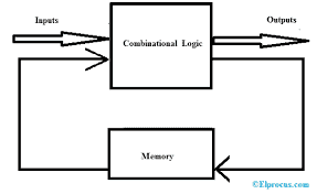
A finite-state machine has a set of finite states, including a starting state, an input alphabet, and a transition function by which a next state is assigned to every pair of a state and an input. Due to its finite states, a finite-state machine has a limited memory. A finite-state machine is an abstract machine that can be in exactly one of a finite number of states at any given time, where a state changes to another in response to some input. Fig. 20.2 shows the finite-state machines discussed in this chapter.

A finite-state machine with no output, also known as a finite-state automaton (FSA), models the changes of states within a system until it achieves one of a collection of desired states. The finite-state automata (the plural of automaton) do not produce output, but they have a set of final states. They recognize input strings that take the starting state to a final state. These machines can be used, for instance, to model ATMs, traffic lights, parity check bits, subway turnstiles, and DVD players. They are also known as language recognizers and thus play a central role in the design and construction of compilers for programming languages. Finite-state automata are categorized into deterministic FSA and nondeterministic FSA.

In a finite-state machine with output, also referred to as a finite-state transducer (FST), each transition has an associated output that either provides some information about the state of the machine or outputs a stream of information as the machine is intended to produce. In a finite-state machine, there are therefore no final states. These machines can be used, for instance, to model vending machines, delay devices, binary adders, pattern finders, network protocols, language and speech recognizers, and spelling and grammar checking. FSTs are categorized into Moore machines and Mealy machines.

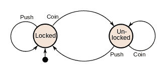
Finite-state machines are represented using either state tables, which are easier to present, or state diagrams (directed graphs with labeled edges), which are easier to understand. In a state diagram for a finite-state machine, the initial state is indicated by means of an arrow that terminates at the initial state but has no initial vertex. Note that every state has a transition for every input. A transition may result in a loop back to the same state. If from some state an input is impossible, then no transition corresponding to that input should be added to the state diagram. A state diagram contains transitions for all possible inputs at each state.

离散数学代写

数学代写|离散数学作业代写discrete mathematics代考|Applications of Trees

树木的应用很多。这里我们只介绍三种可以用树研究和解决的不同问题，即三阶幻方、七局三胜制和霍夫魯编码。
魔方是一个 $n \times n$ 不同的正整数数组，使得每行、每列和主对角线的数字之和相同。请注意，如果数组仅包含正整数 $1,2,3, \ldots, n^2$ ，幻方被认为是正常的。整数 $n$ (在哪里 $n$ 是沿一侧的整数个数) 是正常幻方的阶数，常量和称为幻和，如下所示:
$$
S=\frac{n\left(n^2+1\right)}{2}
$$
任何魔方都可以旋转和反射以产生八个不同的方块。在魔方理论中，所有这些通常被认为是等价的，据说八个这样的方块组成了一个等价类。等效正方形不被视为不同。注意阶数不同的幻方数 (不包括通过旋转和反射得到的) $n=1,2,3,4$, 和 5 是 $1,0,1,880$ ，和 $275,305,224$ ，同时注意到阶数的幻方数 $n \geq 6$ 不完全已知，但可以近似计算。
为了降低数字系统中的存储要求以及数字网络中的传输时间要求，必须对数据进行编码，以便使用更少的位来表示数据符号。为了有效编码 (即，有效数据压缩），更频贁出现的数据符号应该使用较短的比特序列编码，而较长的比特序列应该用于编码很少出现的数据符号。因此，数据符号使用不同数量的比特进行编码。当数据符号的统计数据可用时，霍夫曼码是最佳算法。霍夫曼代码是无前缀 (瞬时) 代码，其中没有代码字是另一个代码字的前缀，因此霍夫曼代码可以使用有根二叉树来表示。
霍夫曼编码算法从一片树开始，每棵树都由一个顶点组成，其中每个顶点显示一个数据符号及其出现概率。必须将顶点按概率递增的顺序排列，即第一个顶点表示可能性最小的符号，最后一个顶点表示可能性最大的符号。在每一步中，我们通过引入一个新根并将权重较大的树作为其子树之一，将权重较小的树作为另一棵子树，将总概率最小的两棵树组合成一棵树。此外，与两个子树相关联的两个概率之和被指定为树的总概率。如有必要，重新排序树的概率，包括新形成的树，使它们仍处于递增顺序。有许多方法可以为一组给定的数据符号及其出现概率提出霍夫睘代码。但是，对于给定的数据符号集，它们每个符号的平均位数都相同。

数学代写|离散数学作业代写discrete mathematics代考|Types of Finite-State Machines

有限状态机是基于由不同状态组成的假设机器的计算数学模型，可用于模拟时序逻辑以表示和控制执行流程。在给定时间只能激活有限状态机的一个状态。完成特定任务的有限状态机本质上是计算机编程，没有具体的执行方法，因为有很多机器可以完成同样的任务。

在有限状态机的上下文中，字符串是元素的有限序列；字母表是一个有限的非空集合，其中包含用于形成字符串的元素；字符串的长度是组成字符串的元素的数量；语言是字母表中所有字符串集合的子集。作为说明一些基本术语的简单示例，图 20.1 显示了具有两个最终状态的有限状态机，即“错误”和“正确”。该机器可以解析长度为 3 的字符串“yes”，同时注意到该字母表由 26 个英文字母组成。

有限状态机具有一组有限状态，包括起始状态、输入字母表和转换函数，通过该转换函数将下一个状态分配给每对状态和输入。由于其有限状态，有限状态机的内存有限。有限状态机是一种抽象机，它可以在任何给定时间恰好处于有限数量的状态中的一个，其中一个状态更改为另一个状态以响应某些输入。图 20.2 显示了本章讨论的有限状态机。

没有输出的有限状态机，也称为有限状态自动机 (FSA)，对系统内的状态变化进行建模，直到它达到所需状态集合中的一个。有限状态自动机（自动机的复数形式）不产生输出，但它们有一组最终状态。它们识别将起始状态变为最终状态的输入字符串。例如，这些机器可用于模拟 ATM、交通信号灯、奇偶校验位、地铁十字转门和 DVD 播放器。它们也被称为语言识别器，因此在编程语言编译器的设计和构建中起着核心作用。有限状态自动机分为确定性 FSA 和非确定性 FSA。

在具有输出的有限状态机（也称为有限状态转换器 (FST)）中，每个转换都有一个关联的输出，该输出要么提供有关机器状态的一些信息，要么输出机器预期的信息流生产。因此，在有限状态机中，没有最终状态。例如，这些机器可用于为自动售货机、延迟设备、二进制加法器、模式查找器、网络协议、语言和语音识别器以及拼写和语法检查建模。FST 分为 Moore 机和 Mealy 机。

有限状态机使用更易于呈现的状态表或更易于理解的状态图（带有标记边的有向图）来表示。在有限状态机的状态图中，初始状态由终止于初始状态但没有初始顶点的箭头表示。请注意，每个状态对每个输入都有一个转换。转换可能会导致返回相同状态的循环。如果从某个状态输入是不可能的，则不应将对应于该输入的转换添加到状态图中。状态图包含每个状态下所有可能输入的转换。

数学代写|离散数学作业代写discrete mathematics代考请认准statistics-lab™

统计代写请认准statistics-lab™. statistics-lab™为您的留学生涯保驾护航。

金融工程代写

金融工程是使用数学技术来解决金融问题。金融工程使用计算机科学、统计学、经济学和应用数学领域的工具和知识来解决当前的金融问题，以及设计新的和创新的金融产品。

非参数统计代写

非参数统计指的是一种统计方法，其中不假设数据来自于由少数参数决定的规定模型；这种模型的例子包括正态分布模型和线性回归模型。

广义线性模型代考

广义线性模型（GLM）归属统计学领域，是一种应用灵活的线性回归模型。该模型允许因变量的偏差分布有除了正态分布之外的其它分布。

术语广义线性模型（GLM）通常是指给定连续和/或分类预测因素的连续响应变量的常规线性回归模型。它包括多元线性回归，以及方差分析和方差分析（仅含固定效应）。

有限元方法代写

有限元方法（FEM）是一种流行的方法，用于数值解决工程和数学建模中出现的微分方程。典型的问题领域包括结构分析、传热、流体流动、质量运输和电磁势等传统领域。

有限元是一种通用的数值方法，用于解决两个或三个空间变量的偏微分方程（即一些边界值问题）。为了解决一个问题，有限元将一个大系统细分为更小、更简单的部分，称为有限元。这是通过在空间维度上的特定空间离散化来实现的，它是通过构建对象的网格来实现的：用于求解的数值域，它有有限数量的点。边界值问题的有限元方法表述最终导致一个代数方程组。该方法在域上对未知函数进行逼近。[1] 然后将模拟这些有限元的简单方程组合成一个更大的方程系统，以模拟整个问题。然后，有限元通过变化微积分使相关的误差函数最小化来逼近一个解决方案。

tatistics-lab作为专业的留学生服务机构，多年来已为美国、英国、加拿大、澳洲等留学热门地的学生提供专业的学术服务，包括但不限于Essay代写，Assignment代写，Dissertation代写，Report代写，小组作业代写，Proposal代写，Paper代写，Presentation代写，计算机作业代写，论文修改和润色，网课代做，exam代考等等。写作范围涵盖高中，本科，研究生等海外留学全阶段，辐射金融，经济学，会计学，审计学，管理学等全球99%专业科目。写作团队既有专业英语母语作者，也有海外名校硕博留学生，每位写作老师都拥有过硬的语言能力，专业的学科背景和学术写作经验。我们承诺100%原创，100%专业，100%准时，100%满意。

随机分析代写

随机微积分是数学的一个分支，对随机过程进行操作。它允许为随机过程的积分定义一个关于随机过程的一致的积分理论。这个领域是由日本数学家伊藤清在第二次世界大战期间创建并开始的。

时间序列分析代写

随机过程，是依赖于参数的一组随机变量的全体，参数通常是时间。随机变量是随机现象的数量表现，其时间序列是一组按照时间发生先后顺序进行排列的数据点序列。通常一组时间序列的时间间隔为一恒定值（如1秒，5分钟，12小时，7天，1年），因此时间序列可以作为离散时间数据进行分析处理。研究时间序列数据的意义在于现实中，往往需要研究某个事物其随时间发展变化的规律。这就需要通过研究该事物过去发展的历史记录，以得到其自身发展的规律。

回归分析代写

多元回归分析渐进（Multiple Regression Analysis Asymptotics）属于计量经济学领域，主要是一种数学上的统计分析方法，可以分析复杂情况下各影响因素的数学关系，在自然科学、社会和经济学等多个领域内应用广泛。

MATLAB代写

MATLAB 是一种用于技术计算的高性能语言。它将计算、可视化和编程集成在一个易于使用的环境中，其中问题和解决方案以熟悉的数学符号表示。典型用途包括：数学和计算算法开发建模、仿真和原型制作数据分析、探索和可视化科学和工程图形应用程序开发，包括图形用户界面构建MATLAB 是一个交互式系统，其基本数据元素是一个不需要维度的数组。这使您可以解决许多技术计算问题，尤其是那些具有矩阵和向量公式的问题，而只需用 C 或 Fortran 等标量非交互式语言编写程序所需的时间的一小部分。MATLAB 名称代表矩阵实验室。MATLAB 最初的编写目的是提供对由 LINPACK 和 EISPACK 项目开发的矩阵软件的轻松访问，这两个项目共同代表了矩阵计算软件的最新技术。MATLAB 经过多年的发展，得到了许多用户的投入。在大学环境中，它是数学、工程和科学入门和高级课程的标准教学工具。在工业领域，MATLAB 是高效研究、开发和分析的首选工具。MATLAB 具有一系列称为工具箱的特定于应用程序的解决方案。对于大多数 MATLAB 用户来说非常重要，工具箱允许您学习和应用专业技术。工具箱是 MATLAB 函数（M 文件）的综合集合，可扩展 MATLAB 环境以解决特定类别的问题。可用工具箱的领域包括信号处理、控制系统、神经网络、模糊逻辑、小波、仿真等。

R语言代写	问卷设计与分析代写
PYTHON代写	回归分析与线性模型代写
MATLAB代写	方差分析与试验设计代写
STATA代写	机器学习/统计学习代写
SPSS代写	计量经济学代写
EVIEWS代写	时间序列分析代写
EXCEL代写	深度学习代写
SQL代写	各种数据建模与可视化代写

数学代写|离散数学作业代写discrete mathematics代考|MPCS50103

Posted on 2023年3月16日2023年3月16日 by statistics-lab

如果你也在怎样代写离散数学discrete mathematics这个学科遇到相关的难题，请随时右上角联系我们的24/7代写客服。

我们提供的离散数学discrete mathematics及其相关学科的代写，服务范围广, 其中包括但不限于:

Statistical Inference 统计推断
Statistical Computing 统计计算
Advanced Probability Theory 高等概率论
Advanced Mathematical Statistics 高等数理统计学
(Generalized) Linear Models 广义线性模型
Statistical Machine Learning 统计机器学习
Longitudinal Data Analysis 纵向数据分析
Foundations of Data Science 数据科学基础

数学代写|离散数学作业代写discrete mathematics代考|MPCS50103

数学代写|离散数学作业代写discrete mathematics代考|Basic Rules of Counting

Suppose a task can be divided into a sequence of $k$ independent subtasks, where $k>0$ is an integer. A subtask is thus carried out regardless of how the other $k-1$ subtasks are done. Assuming $n_1, n_2, \ldots$, and $n_k$ are all positive integers, the first subtask can be carried out in $n_1$ ways, the second subtask in $n_2$ ways, …, and the $k$ th subtask in $n_k$ ways. The fundamental principle of counting, also known as the product rule for counting, states that there is a total of $n_1 \times n_2 \times \ldots \times n_k$ distinct ways to carry out the task consisting of $k$ independent subtasks.

Suppose a task can be done in $k$ mutually exclusive sets of ways, where $k>0$ is an integer. The ways in any one set thus exclude the ways in the other $k-1$ sets. Assuming $n_1, n_2, \ldots$, and $n_k$ are all positive integers, the task can be carried out in one of $n_1$ ways in set 1 , in one of $n_2$ ways in set $2, \ldots$, and in one of $n_k$ ways in set $k$, where the set of $n_1$ ways, the set of $n_2$ ways, $\ldots$, and the set of $n_k$ ways are all pairwise disjoint (mutually exclusive) finite sets. The sum rule for counting, also known as the addition rule for counting, states that there is a total of $n_1+n_2+\ldots+n_k$ distinct ways to carry out the task.

There are also some counting problems that cannot be directly solved using any basic rules of counting. For instance, certain problems that require tree diagrams with asymmetric structures to solve cannot easily use these rules because there are some conditions in these problems that must be met.

The outcomes of a finite sequential experiment can be represented by a tree diagram. A tree structure is a logical way to keep a systematic track of all possibilities in cases in which events occur in sequence but in a finite number of ways. In order to use trees in counting, a branch is used to represent each possible choice, and the leaves, which are the nodes not having other branches starting at them, are used to represent the possible outcomes. The number of branches that originate from a node represents the number of events that can occur, given that the event represented by that node occurs.

数学代写|离散数学作业代写discrete mathematics代考|Random Arrangements and Selections

Permutations and combinations arise when a subset is chosen from a set. In a counting problem, we may determine the number of ways to randomly choose a set of $k$ objects from a set of $n$ distinguishable objects.

An ordered arrangement of $k$ distinguishable objects from a set of $n \geq k$ objects is called a $\boldsymbol{k}$-permutation. In a $k$-permutation, different outcomes are distinguished by the order in which objects are chosen in a sequence. Therefore in a $k$-permutation, both the identity of the objects and their order of arrangement matter, as a permutation results in a list of objects.

As order counts with permutations, some real-life examples of permutations include the order of letters in a word in a natural language, the sequence of digits in a telephone number, books on a shelf in a library, the winners in an Olympic game, multiplication of matrices, and the order of alphanumeric characters in a password.

An unordered selection of $k$ distinguishable objects from a set of $n \geq k$ objects is called a $\boldsymbol{k}$-combination. In a $k$-combination, the identity of objects in a sequence matters but not their order of selection, as a combination results in a group of objects.

As order does not count with combinations, some real-life examples of combinations include multiplication of numbers, putting toppings on a pizza, counting subsets, buying groceries, handshakes among a group of people, taking attendance, voting in an election, answering questions on an exam, games in a round-robin tournament, dice rolled in a dice game, and cards dealt to form a hand in a card game. It is interesting to note that the term combination lock is a misnomer, as the sequence of numbers to unlock matters; in fact, a combination lock should be called a permutation lock.

In a selection with replacement (repetition, substitution), after an object out of $n$ objects is selected, it is returned to the set, and it is thus possible that it will be selected again. In sampling with replacement, the total number of possible outcomes thus remains the same after each selection.

In a selection without replacement, an object, once selected, is not available for future selections. In sampling without replacement, the total number of possible outcomes of each selection depends on the outcomes of previous selections.

离散数学代写

数学代写|离散数学作业代写discrete mathematics代考|Basic Rules of Counting

假设一个任务可以分成一系列 $k$ 独立的子任务，其中 $k>0$ 是一个整数。因此，无论其他任务如何执行，都会执行一个子任务 $k-1$ 子任务完成。假设 $n_1, n_2, \ldots$ ，和 $n_k$ 都是正整数，第一个子任务可以在 $n_1$ 规则，指出总共有 $n_1 \times n_2 \times \ldots \times n_k$ 执行任务的不同方法包括 $k$ 独立的子任务。
假设一个任务可以在 $k$ 互压的方法集，其中 $k>0$ 是一个整数。因此，任何一组中的方式都排除了另一组中的方式 $k-1$ 套。假设 $n_1, n_2, \ldots$ ，和 $n_k$ 都是正整数，任务可以在其中一个进行 $n_1$ set 1 中的方法，其中之一 $n_2$ 集合方式 $2, \ldots$, 并且在其中一个 $n_k$ 集合方式 $k$ ，其中的集合 $n_1$ 方式，集合 $n_2$ 方法， $\ldots$, 和集合 $n_k$ 方式都是成对不相交 (互庍) 的有限集。计数求和规则，也称为计数加法规则，规定总共有 $n_1+n_2+\ldots+n_k$ 执行任务的不同方法。
还有一些计数问题不能用任何基本计数规则直接解决。例如，某些需要非对称结构的树图来解决的问题不能轻易使用这些规则，因为这些问题中有一些必须满足的条件。
有限顺序实验的结果可以用树图表示。在事件按顺序发生但方式有限的情况下，树结构是一种系统地跟踪所有可能性的逻辑方法。为了在计数中使用树，一个分支用于表示每个可能的选择，而叶子是没有其他分支开始的节点，用于表示可能的结果。假定由该节点表示的事件发生，源自该节点的分支数表示可能发生的事件数。

数学代写|离散数学作业代写discrete mathematics代考|Random Arrangements and Selections

当从集合中选择一个子集时，就会出现排列和组合。在计数问题中，我们可以确定随机选择一组的方法的数量 $k$ 一组对象 $n$ 可区分的对象。
的有序排列 $k$ 从一组可区分的对象 $n \geq k$ 对象称为 $\boldsymbol{k}$-排列。在一个 $k$-排列，不同的结果是通过在序列中选择对象的顺序来区分的。因此在一个 $k$-排列，对象的身份及其排列顺序都很重要，因为排列会产生对象列表。
由于顺序与排列有关，一些现实生活中的排列示例包括自然语言中单词中字母的顺序、电话号码中的数字序列、图书馆书架上的书籍、奧林匹克运动会的获胜者，矩阵乘法，以及密码中字母数字字符的顺序。
无序选择 $k$ 从一组可区分的对象 $n \geq k$ 对象称为 $k$-组合。在一个 $k$-组合，序列中对象的身份很重要，但与它们的选择顺序无关，因为组合会产生一组对象。
由于顺序与组合无关，一些现实生活中的组合示例包括数字乘法、在比萨饼上放浇头、计算子集、购买杂货、一群人之间的握手、出席、在选举中投票、回答问题考试、循环赛中的游戏、骰子游戏中烪出的骰子以及纸牌游戏中为组成手牌而发的牌。有趣的是，术语组合锁用词不当，因为解锁的数字序列很重要；其实组合锁应该叫置换锁。
在带有替换（重复、替换）的选择中，从 $n$ 对象被选中，它被返回到集合中，因此它有可能被再次选中。因此，在有放回抽样中，每次选择后可能结果的总数保持不变。
在没有替换的选择中，对象一旦被选中，就不能用于以后的选择。在无放回抽样中，每次选择的可能结果总数取决于先前选择的结果。

统计代写请认准statistics-lab™. statistics-lab™为您的留学生涯保驾护航。

金融工程代写

非参数统计代写

非参数统计指的是一种统计方法，其中不假设数据来自于由少数参数决定的规定模型；这种模型的例子包括正态分布模型和线性回归模型。

广义线性模型代考

广义线性模型（GLM）归属统计学领域，是一种应用灵活的线性回归模型。该模型允许因变量的偏差分布有除了正态分布之外的其它分布。

有限元方法代写

随机分析代写

时间序列分析代写

回归分析代写

MATLAB代写

R语言代写	问卷设计与分析代写
PYTHON代写	回归分析与线性模型代写
MATLAB代写	方差分析与试验设计代写
STATA代写	机器学习/统计学习代写
SPSS代写	计量经济学代写
EVIEWS代写	时间序列分析代写
EXCEL代写	深度学习代写
SQL代写	各种数据建模与可视化代写

数学代写|离散数学作业代写discrete mathematics代考|MATH200

Posted on 2023年3月16日2023年3月16日 by statistics-lab

如果你也在怎样代写离散数学discrete mathematics这个学科遇到相关的难题，请随时右上角联系我们的24/7代写客服。

我们提供的离散数学discrete mathematics及其相关学科的代写，服务范围广, 其中包括但不限于:

Statistical Inference 统计推断
Statistical Computing 统计计算
Advanced Probability Theory 高等概率论
Advanced Mathematical Statistics 高等数理统计学
(Generalized) Linear Models 广义线性模型
Statistical Machine Learning 统计机器学习
Longitudinal Data Analysis 纵向数据分析
Foundations of Data Science 数据科学基础

数学代写|离散数学作业代写discrete mathematics代考|MATH200

数学代写|离散数学作业代写discrete mathematics代考|Solving Linear Nonhomogeneous Recurrence Relations

A linear nonhomogeneous recurrence relation with constant coefficients is in the following form:
$$
a_n=c_1 a_{n-1}+c_2 a_{n-2}+\ldots+c_k a_{k-n}+f(n),
$$
where $c_1, c_2, \ldots, c_k$ are real numbers, $c_k \neq 0$, and $f(n)$ is a function of the variable $n$ only. The recurrence relation
$$
a_n=c_1 a_{n-1}+c_2 a_{n-2}+\ldots+c_k a_{k-n}
$$ which is known in this context as the associated homogeneous recurrence relation with constant coefficients, provides a solution, denoted by $a_n^{(h)}$, to the linear nonhomogeneous recurrence relation with constant coefficients. The general solution of the linear nonhomogeneous recurrence relation with constant coefficients is then given by
$$
a_n=a_n^{(h)}+a_n^{(p)}
$$
where $a_n^{(p)}$ is called a particular solution. There is no general method to find a particular solution for every function $f(n)$. However, when $f(n)$ is a polynomial in $n$ and the power of a constant, a particular solution can be rather easily found. Suppose $f(n)$ is as follows:
$$
f(n)=\left(b_t n^t+b_{t-1} n^{t-1}+\ldots+b_1 n+b_0\right) \alpha^n
$$
where $b_0, b_1, \ldots, b_t$ and $\alpha$ are real numbers. Then a particular solution has the following form:
$$
a_n^{(p)}=g(n)\left(e_t n^t+e_{t-1} n^{t-1}+\ldots+e_1 n+e_0\right) \alpha^n
$$
where $e_0, e_1, \ldots, e_t$ are some constants to be determined using the initial conditions. If $\alpha$ is not a root of the characteristic equation of the associated linear nonhomogeneous recurrence relation with constant coefficient, then $g(n)=1$. If $\alpha$ is a root of this characteristic equation and its multiplicity is $m$, then $g(n)=n^m$.

数学代写|离散数学作业代写discrete mathematics代考|Solving Recurrence Relations Using Generating Functions

Generating functions is a powerful and efficient tool to solve many types of problems, such as advanced counting, calculating the probability of discrete random variables, and solving recurrence relations. The solution to a recurrence relation with its initial conditions can be found when an explicit formula for the associated generating function is determined.

Generating functions can translate the terms of a sequence as coefficients of powers of a variable $z$ in a formal power series. The generating function for the sequence $a_0, a_1, a_2, \ldots$ of real numbers is the following infinite series:
$$
G(z) \triangleq a_0+a_1 z+a_2 z^2+\ldots=\sum_{n=0}^{\infty} a_n z^n
$$

Note that two generating functions can be added and multiplied as follows:
$$
\left{\begin{array} { l }
{ G ( z ) = a _ { 0 } + a _ { 1 } z + a _ { 2 } z ^ { 2 } + \ldots = \sum _ { n = 0 } ^ { \infty } a _ { n } z ^ { n } } \
{ F ( z ) = b _ { 0 } + b _ { 1 } z + b _ { 2 } z ^ { 2 } + \ldots = \sum _ { n = 0 } ^ { \infty } b _ { n } z ^ { n } }
\end{array} \rightarrow \left{\begin{array}{l}
G(z)+F(z)=\sum_{n=0}^{\infty}\left(a_n+b_n\right) z^n \
F(z) G(z)=\sum_{n=0}^{\infty}\left(\sum_{j=0}^n b_j a_{n-j}\right) z^n
\end{array}\right.\right.
$$
Table 14.2 presents some useful generating functions. In addition, the following highlights shifting a generating function and differentiating a generating function as two important mathematical operations that can help solve recurrence relations:
$$
z^m G(z)=\sum_{n=0}^{\infty} a_n z^{n+m}=\sum_{n=m}^{\infty} a_{n-m} z^n
$$
and
$$
G^{\prime}(z)=\sum_{n=1}^{\infty} n a_n z^{n-1}
$$
It is imperative to highlight that the goal is to use the generating function and its properties to a recurrence relation in order to find $G(z)$ in the form of a single summation, of course after some mathematical manipulation, and then to determine the sequence $\left{a_n\right}$ by using the definition of the generating function.

离散数学代写

数学代写|离散数学作业代写discrete mathematics代考|Solving Linear Nonhomogeneous Recurrence Relations

具有常系数的线性非齐次递推关系具有以下形式:
$$
a_n=c_1 a_{n-1}+c_2 a_{n-2}+\ldots+c_k a_{k-n}+f(n)
$$
在哪里 $c_1, c_2, \ldots, c_k$ 是实数， $c_k \neq 0$ ，和 $f(n)$ 是变量的函数 $n$ 仅有的。递归关系
$$
a_n=c_1 a_{n-1}+c_2 a_{n-2}+\ldots+c_k a_{k-n}
$$
在这种情况下被称为具有常数系数的相关齐次递归关系，提供了一个解决方案，表示为 $a_n^{(h)}$ ，到具有常系数的线性非齐次递归关系。常系数线性非齐次递归关系的通解由下式给出
$$
a_n=a_n^{(h)}+a_n^{(p)}
$$
在哪里 $a_n^{(p)}$ 称为特解。没有通用的方法可以为每个功能找到特定的解决方案 $f(n)$. 然而，当 $f(n)$ 是一个多项式 $n$ 和常数的力量，可以很容易地找到特定的解决方案。认为 $f(n)$ 如下:
$$
f(n)=\left(b_t n^t+b_{t-1} n^{t-1}+\ldots+b_1 n+b_0\right) \alpha^n
$$
在哪里 $b_0, b_1, \ldots, b_t$ 和 $\alpha$ 是实数。那么一个特定的解决方案具有以下形式:
$$
a_n^{(p)}=g(n)\left(e_t n^t+e_{t-1} n^{t-1}+\ldots+e_1 n+e_0\right) \alpha^n
$$
在哪里 $e_0, e_1, \ldots, e_t$ 是一些要使用初始条件确定的常数。如果 $\alpha$ 不是关联的常系数线性非齐次递推关系的特征方程的根，则 $g(n)=1$. 如果 $\alpha$ 是这个特征方程的根，它的重数是 $m$ ，然后 $g(n)=n^m$.

数学代写|离散数学作业代写discrete mathematics代考|Solving Recurrence Relations Using Generating Functions

生成函数是解决许多类型问题的强大而有效的工具，例如高级计数、计算离散随机变量的概率以及求解递归关系。当确定相关生成函数的显式公式时，可以找到具有初始条件的递归关系的解。
生成函数可以将序列的项转换为变量的幂系数 $z$ 在一个正式的幂级数中。序列的生成函数 $a_0, a_1, a_2, \ldots$ 实数的无穷级数如下:
$$
G(z) \triangleq a_0+a_1 z+a_2 z^2+\ldots=\sum_{n=0}^{\infty} a_n z^n
$$
请注意，两个生成函数可以按如下方式相加和相乘:
$\$ \$$
Veft {
$$
G(z)=a_0+a_1 z+a_2 z^2+\ldots=\sum_{n=0}^{\infty} a_n z^n F(z)=b_0+b_1 z+b_2 z^2+\ldots=\sum_{n=0}^{\infty} b_n z^n
$$
右箭头 $\backslash$ 左 {
$$
G(z)+F(z)=\sum_{n=0}^{\infty}\left(a_n+b_n\right) z^n F(z) G(z)=\sum_{n=0}^{\infty}\left(\sum_{j=0}^n b_j a_{n-j}\right) z^n
$$
是的是的。
Table14.2presentssomeuse fulgenerating functions. Inaddition, the followinghighligh
$z^{\wedge} m \mathrm{G}(z)=\backslash$ sum_{n=0 $\left{\wedge{\right.$ infty $}$ a_n $z^{\wedge}{n+m}=\mid$ sum_${n=m} \wedge{$ linfty $}$ a_ ${n m} z^{\wedge} n$
and
$G^{\wedge}{\backslash \operatorname{prime}}(z)=\backslash$ sum_{n=1}^{linfty} $n$ a_n $z^{\wedge}{n-1} \$ \$$ 必须强调的是，目标是使用生成函数
及其
性质到递归关系，以便找到 $G(z)$ 以单个求和的形式，当然是经过一些数学运算，然后确定序列
$\backslash$ 左 ${$ a_n\右 $}$ 通过使用生成函数的定义。

统计代写请认准statistics-lab™. statistics-lab™为您的留学生涯保驾护航。

金融工程代写

非参数统计代写

非参数统计指的是一种统计方法，其中不假设数据来自于由少数参数决定的规定模型；这种模型的例子包括正态分布模型和线性回归模型。

广义线性模型代考

广义线性模型（GLM）归属统计学领域，是一种应用灵活的线性回归模型。该模型允许因变量的偏差分布有除了正态分布之外的其它分布。

有限元方法代写

随机分析代写

时间序列分析代写

回归分析代写

MATLAB代写

R语言代写	问卷设计与分析代写
PYTHON代写	回归分析与线性模型代写
MATLAB代写	方差分析与试验设计代写
STATA代写	机器学习/统计学习代写
SPSS代写	计量经济学代写
EVIEWS代写	时间序列分析代写
EXCEL代写	深度学习代写
SQL代写	各种数据建模与可视化代写

数学代写|离散数学作业代写discrete mathematics代考|MPCS50103

Posted on 2023年3月6日2023年3月6日 by statistics-lab

如果你也在怎样代写离散数学discrete mathematics这个学科遇到相关的难题，请随时右上角联系我们的24/7代写客服。

我们提供的离散数学discrete mathematics及其相关学科的代写，服务范围广, 其中包括但不限于:

Statistical Inference 统计推断
Statistical Computing 统计计算
Advanced Probability Theory 高等概率论
Advanced Mathematical Statistics 高等数理统计学
(Generalized) Linear Models 广义线性模型
Statistical Machine Learning 统计机器学习
Longitudinal Data Analysis 纵向数据分析
Foundations of Data Science 数据科学基础

数学代写|离散数学作业代写discrete mathematics代考|Binary Operations

The computational methods of binary arithmetic are analogous to those of decimal arithmetic. In binary arithmetic, the number $2=(10)_2$ in binary notation plays a role similar to that of the number 10 in decimal arithmetic.

In binary addition, carryovers of binary addition are performed in the same manner as in decimal addition. We thus have $0+0=0,0+1=1,1+0=1$, and $1+1=$ 10, all in base 2.

The binary multiplication is carried out by multiplying the multiplicand by one bit of the multiplier at a time and the result of the partial product for each bit is placed in such a manner that the least significant bit is under the corresponding multiplier bit. Finally, the partial products are added to get the complete product.

In binary subtraction, like decimal subtraction, it may be necessary to borrow. However, the method introduced here is based on not using borrow, as one’s complement and two’s complement of binary numbers are used to perform subtraction.

The one’s complement of a binary number can be obtained by inverting each bit from 1 to 0 or from 0 to 1 . For example, one’s complement of the binary number 110010 is 001101 . To get two’s complement of a binary number is to first obtain the one’s complement of the number and then add 1 to the least significant bit. For example, two’s complement of the binary number 10010 is $01101+00001=01110$.
The binary subtraction can be carried out using the following steps:
(i) Find the two’s complement of the subtrahend, and then add it to the minuend.
(ii) If the final carryover of the sum is 1 , it is dropped and the result is positive, and if there is no carryover, the two’s complement of the sum will be the result and it is negative. The binary division is similar to that employed in the decimal system. However, in the case of binary numbers, the operation is simpler because the quotient can have either 1 or 0 depending upon the divisor.

Fermat’s little theorem, which is very useful in computing the remainder modulo prime of large powers of integers, can be expressed in terms of congruences. Fermat’s little theorem states that if $p$ is prime and $a$ is an integer not divisible by $p$, then
$$
a^{p-1} \equiv 1(\bmod p) \leftrightarrow a^{p-1} \bmod p=1
$$
or equivalently,
$$
a^p \equiv a(\bmod p) \leftrightarrow a^p \bmod p=a
$$

数学代写|离散数学作业代写discrete mathematics代考|Classical Cryptography

Cryptography is about making secret communication to make messages secure in the presence of adversaries. By encryption, an original message, called plaintext, is transformed into a coded message, called ciphertext. This transformation is performed before the plaintext is transmitted or stored. The reverse process is called decryption and is performed after the ciphertext is received or retrieved. The algorithm used for encryption and decryption is often called a cipher, and the process of encryption and decryption requires a secret key. A key is a number (value) that the cipher operates on, without which the unauthorized parties must not be able to recover the original message.

In classical cryptography, symbols, characters, letters, and digits were directly manipulated with the sole goal to provide secrecy through obscurity. It appears that encrypted messages were first developed in ancient Egypt using disordered hieroglyphics, which consisted of visual symbols and characters. There were then other forms of message concealment, which were developed by the Greeks, namely stenography, through which a secret message was hidden within an ordinary nonsecret message, and by the Spartans, namely scytale, by which a narrow strip of parchment was wound on a rod and the message written across the adjoining edges.

A well-known classical cryptography technique, which was developed by Romans, was the Caesar cipher, a simple encryption method based on substitution. The Caesar cipher shifts each letter in the alphabet by three letters forward, for instance, the letter $G$ becomes $J$. It thus requires a letter three places further along, while wrapping the letters at the end of the alphabet around to the letters at the beginning of the alphabet that is $X$ wraps around to $\mathrm{A}, \mathrm{Y}$ to $\mathrm{B}$, and $\mathrm{Z}$ to $\mathrm{C}$.

Mathematically described, in the Caesar cipher, each letter is coded by its position relative to others. To this effect, an integer $i \in{0,1, \ldots, 24,25}$ replaces a letter whose position in the alphabet ${\mathrm{A}, \mathrm{B}, \ldots, \mathrm{Y}, \mathrm{Z}}$ is the $i$ th; for instance, $\mathrm{D}$ is the fourth letter in the alphabet, that is $i=3, \mathrm{D}$ is thus replaced by 3 . Assuming the nonnegative integer $p \leq 25$, the functions providing the encrypted message and the decrypted message are $f(p)=(p+3) \bmod 26$ and $f^{-1}(p)=(p-3) \bmod 26$, respectively.

A slight generalization of the Caesar, cipher called the shift cipher or the additive cipher, is when 3 is replaced by the integer $b$, called a key. In other words, the numerical equivalent of each letter is shifted by $b$, thus yielding the following functions:
$$
\left{\begin{array}{l}
\text { Encryption } \rightarrow f(p)=(p+b) \bmod 26 \
\text { Decryption } \rightarrow f^{-1}(p)=(p-b) \bmod 26
\end{array}\right.
$$

离散数学代写

数学代写|离散数学作业代写discrete mathematics代考|Binary Operations

二进制算术的计算方法类似于十进制算术。在二进制算术中，数 $2=(10)_2$ 在二进制表示法中，它的作用类似于十进制算术中数字 10 的作用。
在二进制加法中，二进制加法的结转以与十进制加法相同的方式执行。我们因此有 $0+0=0,0+1=1,1+0=1$ ，和 $1+1=10$ ，全部在基地 2 。
二进制乘法是通过将被乘数一次乘以乘数的一位来进行的，并且将每一位的部分积的结果以最低有效位在对应的乘数位之下的方式放置。最后将部分产品相加得到完整的产品。
在二进制减法中，和十进制减法一样，可能需要借位。但是，这里介绍的方法是在不使用借位的基础上的，因为是用二进制数的一个补码和二进制补码来进行减法运算。
二进制数的补码可以通过将每个位从 1 反转为 0 或从 0 反转为 1 来获得。例如，二进制数 110010 的补码是 001101 。求一个二进制数的补码就是先求这个数的补码，然后在最低位加 1. 例如，二进制数 10010 的补码是 $01101+00001=01110$.
二进制减法可以使用以下步骙进行:
(i) 找到减数的二进制补码，然后将其与被减数相加。
(ii) 如果和的最终结转为 1 ，则将其丢弃，结果为正，如果没有结转，则和的二进制补码为结果，结果为负。二进制除法类似于十进制系统中使用的除法。然而，在二进制数的情况下，操作更简单，因为商可以是 1 或 0 ，具体取决于除数。
费马小定理在计算大整数次幂的余数模素数时非常有用，可以用同余来表示。费马小定理指出，如果 $p$ 是质数和 $a$ 是一个不能被整除的整数 $p$ ，然后
$$
a^{p-1} \equiv 1(\bmod p) \leftrightarrow a^{p-1} \bmod p=1
$$
或者等价地，
$$
a^p \equiv a(\bmod p) \leftrightarrow a^p \bmod p=a
$$

数学代写|离散数学作业代写discrete mathematics代考|Classical Cryptography

密码学是关于进行秘密通信以在对手存在的情况下确保消息安全。通过加密，称为明文的原始消息被转换为称为密文的编码消息。这种转换是在传输或存储明文之前执行的。相反的过程称为解密，在收到或检索到密文后执行。用于加密和解密的算法通常称为密码，加密和解密的过程需要密钥。密钥是密码操作所依据的数字（值），没有它，末经授权的方就不能恢复原始消息。
在经典密码学中，符号、字符、字母和数字被直接操纵，其唯一目标是通过模糊提供保密性。加密消息似乎最早是在古埃及使用无序的象形文字开发的，它由视觉符号和字符组成。然后还有其他形式的消息隐藏，由希腊人开发，即速记术，通过它可以将秘密消息隐藏在普通的非秘密消息中，以及由斯巴达人开发的称为 scytale 的方法，通过这种方法，将一条狭窄的羊皮纸缠绕在一根杆和写在相邻边缘的信息。
由罗马人开发的一种著名的经典密码技术是凯措密码，这是一种基于替换的简单加密方法。凯撒密码将字母表中的每个字母向前移动三个字母，例如，字母 $G$ 成为 $J$. 因此，它需要一个字母再往前三个位置，同时将字母表末尾的字母环绕到字母表开头的字母，即 $X$ 环绕到 $\mathrm{A}, \mathrm{Y}$ 到 $\mathrm{B}$ ，和Z到C.
从数学上描述，在凯撒密码中，每个字母都根据其相对于其他字母的位置进行编码。为此，个整数 $i \in 0,1, \ldots, 24,25$ 替换在字母表中位置的字母 $\mathrm{A}, \mathrm{B}, \ldots, \mathrm{Y}, \mathrm{Z}$ 是个 $i$ th; 例如， D是字母表中的第四个字母，即 $i=3, \mathrm{D}$ 因此被 3 取代。假设非负整数 $p \leq 25$ ，提供加密消息和解密消息的函数是 $f(p)=(p+3) \bmod 26$ 和 $f^{-1}(p)=(p-3) \bmod 26$ ，分别。
凯撒密码的一种略微概括，称为移位密码或加法密码，是将 3 替换为整数 $b$ ，称为钥匙。换句话说，每个字母的数字等价物移动了b，从而产生以下功能：
$\$ \$$
Veft {
Encryption $\rightarrow f(p)=(p+b) \bmod 26$ Decryption $\rightarrow f^{-1}(p)=(p-b) \bmod 26$
、正确的。

统计代写请认准statistics-lab™. statistics-lab™为您的留学生涯保驾护航。

金融工程代写

非参数统计代写

非参数统计指的是一种统计方法，其中不假设数据来自于由少数参数决定的规定模型；这种模型的例子包括正态分布模型和线性回归模型。

广义线性模型代考

广义线性模型（GLM）归属统计学领域，是一种应用灵活的线性回归模型。该模型允许因变量的偏差分布有除了正态分布之外的其它分布。

有限元方法代写

随机分析代写

时间序列分析代写

回归分析代写

MATLAB代写

R语言代写	问卷设计与分析代写
PYTHON代写	回归分析与线性模型代写
MATLAB代写	方差分析与试验设计代写
STATA代写	机器学习/统计学习代写
SPSS代写	计量经济学代写
EVIEWS代写	时间序列分析代写
EXCEL代写	深度学习代写
SQL代写	各种数据建模与可视化代写

数学代写|离散数学作业代写discrete mathematics代考|CS3653

Posted on 2023年3月6日2023年3月6日 by statistics-lab

如果你也在怎样代写离散数学discrete mathematics这个学科遇到相关的难题，请随时右上角联系我们的24/7代写客服。

我们提供的离散数学discrete mathematics及其相关学科的代写，服务范围广, 其中包括但不限于:

Statistical Inference 统计推断
Statistical Computing 统计计算
Advanced Probability Theory 高等概率论
Advanced Mathematical Statistics 高等数理统计学
(Generalized) Linear Models 广义线性模型
Statistical Machine Learning 统计机器学习
Longitudinal Data Analysis 纵向数据分析
Foundations of Data Science 数据科学基础

数学代写|离散数学作业代写discrete mathematics代考|Congruences

Modular arithmetic is an important aspect of divisibility. Some trivial examples of modular arithmetic may include that 2 hours and 20 minutes after $7: 45$ is $10: 05$ and that 17 days after a Tuesday is a Friday. Congruences have many applications, such as generating pseudorandom numbers for computer simulations, generating parity check bits to detect and correct errors in digital transmission and storage, storing huge records in a rather small table and retrieving them quickly, and above all modern cryptography. Assuming $a$ and $b$ are integers and $m$ is a positive integer, $\boldsymbol{a}$ is congruent to $\boldsymbol{b}$ modulo $\boldsymbol{m}$, denoted by $a \equiv b(\bmod m)$, if $m$ divides $a-b$, that is, $m \mid(a-b)$ or equivalently $a-b=k m$ for some integer $k$. We say that $a \equiv b(\bmod m)$ is a congruence and that $m$ is its modulus. Congruence is an equivalence relation, as for integers $a, b, c$, and $m>0$, we have

Reflexivity property: $a \equiv a(\bmod m)$.
Symmetry property: $a \equiv b(\bmod m) \rightarrow b \equiv a(\bmod m)$.

Transitivity property: $a \equiv b(\bmod m)$ and $b \equiv c(\bmod m) \rightarrow a \equiv c(\bmod m)$.
While noting that the notation $a \equiv b(\bmod m)$ represents a relation on the set of integers and the notation $a \bmod m=b$ represents a function, we have
$$
a \equiv b(\bmod m) \text { if and only if } a \bmod m=b \bmod m
$$
where $a, b$, and $m>0$ are all integers. In addition, for integers $a, b, c, d, n$, and $m>0$, we have
$$
\left{\begin{array} { l }
{ a \equiv b ( \operatorname { m o d } m ) } \
{ c \equiv d ( \operatorname { m o d } m ) }
\end{array} \rightarrow \left{\begin{array}{l}
a+c \equiv b+d(\bmod m) \
a-c \equiv b-d(\bmod m) \
a c \equiv b d(\bmod m) \
a^n \equiv b^n(\bmod m)
\end{array}\right.\right.
$$
Note that $a c \equiv b c(\bmod m)$ does not imply $a \equiv b(\bmod m)$ unless $\operatorname{gcd}(c, m)=1$. For instance, $85 \equiv 55(\bmod 10)$ does not yield $17 \equiv 11(\bmod 10)$ as $\operatorname{gcd}(5,10) \neq 1$, but $85 \equiv 55(\bmod 6)$ does yield $17 \equiv 11(\bmod 6)$ as $\operatorname{gcd}(5,6)=1$.

数学代写|离散数学作业代写discrete mathematics代考|Representations of Integers

Any positive integer $a$ can be uniquely represented in the following form:
$$
a=a_k\left(b^k\right)+a_{k-1}\left(b^{k-1}\right)+\ldots+a_1(b)+a_0,
$$ where $b$, known as the base, is an integer greater than $1, k$ is a nonnegative integer, $a_0$, $a_1, \ldots, a_k$ are nonnegative integers less than $b$, and $a_k \neq 0$. This representation of the integer $a$ is called the base-b expansion of $a$, which can be denoted by $\left(a_k a_{k-1} \ldots a_1 a_0\right)_b$. Note that $b$ represents the number of different symbols that can be used in a numeral system. There are various representations of integers, including the following expansions:

Decimal expansions: $b=10 \rightarrow 10$ symbols ${0,1,2,3,4,5,6,7,8,9}$.
Binary expansions: $b=2 \rightarrow 2$ symbols ${0,1}$.
Octal expansions: $b=8 \rightarrow 8$ symbols ${0,1,2,3,4,5,6,7}$.
Hexadecimal expansions: $b=16 \rightarrow 16$ symbols ${0,1,2,3,4,5,6,7,8,9$, A, B, $\mathrm{C}, \mathrm{D}, \mathrm{E}, \mathrm{F}}$

Note that the subscript 10 representing the base in the decimal expansion is commonly omitted, and the binary expansion of an integer is just a bit string. The binary expansion is widely used in digital devices and networks to represent and carry out arithmetic with integers. The hexadecimal system is commonly used to describe locations in memory because it can represent every byte ( 8 bits) as two consecutive hexadecimal digits instead of the eight digits that would be required by the binary expansion. While noting that in hexadecimal expansions, $\mathrm{A}=10, \mathrm{~B}=11, \mathrm{C}=12, \mathrm{D}=13, \mathrm{E}=14$, and $\mathrm{F}=15$, it is much easier to read hexadecimal numbers than binary numbers.

离散数学代写

数学代写|离散数学作业代写discrete mathematics代考|Congruences

模运算是可除性的一个重要方面。模运算的一些简单示例可能包括 2 小时 20 分钟后 $7: 45$ 是 $10: 05$ 星期二之后的 17 天是星期五。同余有许多应用，例如为计算机模拟生成伪随机数，生成奇偶校验位以检贬和纠正数字传输和存储中的错误，将大量记录存储在一个相当小的表中并快速检索它们，最重要的是现代密码学。假设 $a$ 和 $b$ 是整数和 $m$ 是正整数， $\boldsymbol{a}$ 是一致的 $\boldsymbol{b}$ 模块 $\boldsymbol{m}$ ，表示为 $a \equiv b(\bmod m)$ ，如果 $m$ 分裂 $a-b$ ，那是， $m \mid(a-b)$ 或等价地 $a-b=k m$ 对于某个整数 $k$. 我们说 $a \equiv b(\bmod m)$ 是全等的 $m$ 是它的模数。同余是等价关系，对于整数 $a, b, c$ ，和 $m>0$ ，我们有

自反性性质： $a \equiv a(\bmod m)$.
对称性: $a \equiv b(\bmod m) \rightarrow b \equiv a(\bmod m)$.
传递性: $a \equiv b(\bmod m)$ 和 $b \equiv c(\bmod m) \rightarrow a \equiv c(\bmod m)$. 同时注意到符号 $a \equiv b(\bmod m)$ 表示整数集和符号上的关系 $a \bmod m=b$ 代表一个函数，我们有
$$
a \equiv b(\bmod m) \text { if and only if } a \bmod m=b \bmod m
$$
在哪里 $a, b$ ，和 $m>0$ 都是整数。此外，对于整数 $a, b, c, d, n$ ，和 $m>0$ ，我们有 $\$ \$$
Veft {
$$
a \equiv b(\bmod m) c \equiv d(\bmod m)
$$
右箭头左 {
$$
a+c \equiv b+d(\bmod m) a-c \equiv b-d(\bmod m) a c \equiv b d(\bmod m) a^n \equiv b^n(\bmod
$$
是的是的。 $\$ \$$
注意 $a c \equiv b c(\bmod m)$ 并不意味着 $a \equiv b(\bmod m)$ 除非 $\operatorname{gcd}(c, m)=1$. 例如， $85 \equiv 55(\bmod 10)$ 不屈服 $17 \equiv 11(\bmod 10)$ 作为 $\operatorname{gcd}(5,10) \neq 1$ ，但 $85 \equiv 55(\bmod 6)$ 确实产生 $17 \equiv 11(\bmod 6)$ 作为 $\operatorname{gcd}(5,6)=1$.
费马小定理在计算大整数次冪的余数模素数时非常有用，可以用同余来表示。费马小定理指出，如果 $p$ 是质数和 $a$ 是一个不能被整除的整数 $p$ ，然后
$$
a^{p-1} \equiv 1(\bmod p) \leftrightarrow a^{p-1} \bmod p=1
$$
或者等价地，
$$
a^p \equiv a(\bmod p) \leftrightarrow a^p \bmod p=a
$$

数学代写|离散数学作业代写discrete mathematics代考|Representations of Integers

任何正整数 $a$ 可以用以下形式唯一表示:
$$
a=a_k\left(b^k\right)+a_{k-1}\left(b^{k-1}\right)+\ldots+a_1(b)+a_0,
$$
在哪里 $b$ ，称为基数，是一个大于 $1, k$ 是一个非负整数， $a_0, a_1, \ldots, a_k$ 是小于的非负整数 $b$ ，和 $a_k \neq 0$. 整数的这种表示 $a$ 称为 $\mathrm{b}$ 基展开 $a$, 可以表示为 $\left(a_k a_{k-1} \ldots a_1 a_0\right)_b$. 注意 $b$ 表示可以在数字系统中使用的不同符号的数量。整数有多种表示形式，包括以下扩展:

十进制展开: $b=10 \rightarrow 1$ 符号 $0,1,2,3,4,5,6,7,8,9$.
-二进制扩展: $b=2 \rightarrow 2$ 符号 0,1 .
八进制扩展: $b=8 \rightarrow 8$ 符号 $0,1,2,3,4,5,6,7$.
十六进制展开: $b=16 \rightarrow 16$ 符号 $0,1,2,3,4,5,6,7,8,9 \$, A, B, \$ \mathrm{C}, \mathrm{D}, \mathrm{E}, \mathrm{F}$
注意十进制展开中表示基数的下标 10 一般省略，整数的二进制展开就是一个位串。二进制扩展广泛用于数字设备和网络中，以表示和执行整数运算。十六进制系统通常用于描述内存中的位置，因为它可以将每个字节 (8 位) 表示为两个连续的十六进制数字，而不是二进制扩展所需的八个数字。虽然注意到在十六进制扩展中，
$\mathrm{A}=10, \mathrm{~B}=11, \mathrm{C}=12, \mathrm{D}=13, \mathrm{E}=14$ ，和 $\mathrm{F}=15$ ，读取十六进制数比读取二进制数要容易得多。

统计代写请认准statistics-lab™. statistics-lab™为您的留学生涯保驾护航。

金融工程代写

非参数统计代写

非参数统计指的是一种统计方法，其中不假设数据来自于由少数参数决定的规定模型；这种模型的例子包括正态分布模型和线性回归模型。

广义线性模型代考

广义线性模型（GLM）归属统计学领域，是一种应用灵活的线性回归模型。该模型允许因变量的偏差分布有除了正态分布之外的其它分布。

有限元方法代写

随机分析代写

时间序列分析代写

回归分析代写

MATLAB代写

R语言代写	问卷设计与分析代写
PYTHON代写	回归分析与线性模型代写
MATLAB代写	方差分析与试验设计代写
STATA代写	机器学习/统计学习代写
SPSS代写	计量经济学代写
EVIEWS代写	时间序列分析代写
EXCEL代写	深度学习代写
SQL代写	各种数据建模与可视化代写

数学代写|离散数学作业代写discrete mathematics代考|MATH200

Posted on 2023年3月6日2023年3月6日 by statistics-lab

如果你也在怎样代写离散数学discrete mathematics这个学科遇到相关的难题，请随时右上角联系我们的24/7代写客服。

我们提供的离散数学discrete mathematics及其相关学科的代写，服务范围广, 其中包括但不限于:

Statistical Inference 统计推断
Statistical Computing 统计计算
Advanced Probability Theory 高等概率论
Advanced Mathematical Statistics 高等数理统计学
(Generalized) Linear Models 广义线性模型
Statistical Machine Learning 统计机器学习
Longitudinal Data Analysis 纵向数据分析
Foundations of Data Science 数据科学基础

数学代写|离散数学作业代写discrete mathematics代考|Greatest Common Divisors and Least Common Multiples

The greatest common divisor (gcd) of two nonzero integers $a$ and $b$, denoted by $\operatorname{gcd}(a, b)$, is the largest integer $d$ such that $d \mid a$ and $d \mid b$, except that $\operatorname{gcd}(0,0)=0$. Note that if $\operatorname{gcd}(a, b)=d$, then $\operatorname{gcd}\left(\frac{a}{d}, \frac{b}{d}\right)=1$. For instance, the set of divisors of 24 is ${1,2,3,4,6,8,12,24}$ and the set of divisors of 42 is ${1,2,3,6,7,14,21}$. Because the set of common divisors is ${1,2,3,6}$, we have $\operatorname{gcd}(24,42)=6$, also $\operatorname{gcd}\left(\frac{24}{6}, \frac{42}{6}\right)=\operatorname{gcd}(4,7)=1$

The integers $a$ and $b$ are relatively prime if their gad is 1 . For instance, neither 15 nor 16 is prime; however, 15 and 16 are relatively prime, as their gcd is 1 . In addition, integers are called pairwise relatively prime if the gcd of any two integers is 1 . For instance, none of the integers 25,26 , and 27 is prime, yet they are pairwise relatively prime.

The gcd of two nonzero integers exists if the set of their common divisors is nonempty and finite. The methods to determine the gcd of two integers $a$ and $b$ are as follows:

Brute-force method: First, find all the positive divisors of each integer, then determine the set of all common divisors of both integers, and finally select the largest common divisor in the set.

数学代写|离散数学作业代写discrete mathematics代考|Divisibility Test

A divisibility test is a quick way to determine whether an integer, called dividend, is divisible by a smaller integer, called divisor, without performing the division. The test is usually based on the examination of the digits of the dividend in a way that solely depends on what the divisor is. Consider an integer $a$ with $n$ digits $\left{a_{n-1}, a_{n-2}, \ldots, a_1, a_0\right}$ whose decimal representation is then as follows:
$$
a=a_{n-1}\left(10^{n-1}\right)+a_{n-2}\left(10^{n-2}\right)+\ldots+a_1\left(10^1\right)+a_0\left(10^0\right) .
$$
Note that $a_0$ is the least significant digit and $a_{n-1}$ is the most significant digit. As an example, we have $71524=7 \times\left(10^4\right)+1 \times\left(10^3\right)+5 \times\left(10^2\right)+2 \times\left(10^1\right)+$ $4 \times\left(10^{\circ}\right)$, where the least significant digit is 4 and the most significant digit is 7 .
The divisibility rules for dividing an integer $a$ by the integers $1,2,3,4,5,6,7,8,9$, or 10 are as follows:

Divisibility by 1: $1 \mid a \rightarrow$ No special condition on the coefficients $a_{n-1}, a_{n-2}, \ldots, a_0$ (i.e., every integer is divisible by 1 ).
Divisibility by 2: $2 \mid a \rightarrow a \bmod 2=a_0 \bmod 2=0 \rightarrow a_0 \in{0,2,4,6,8}$ (i.e., the least significant digit must be even).
Divisibility by 3: $3 \mid a \rightarrow a \bmod 3=\left(a_{n-1}+a_{n-2}, \ldots+a_0\right) \bmod 3=0$ (i.e., the sum of all digits must be divisible by 3 ).
Divisibility by 4: $4 \mid a \rightarrow a \bmod 4=\left(a_1\left(10^1\right)+a_0\left(10^0\right)\right) \bmod 4=0$ (i.e., the number representing the last two digits must be divisible by 4).
Divisibility by 5: $5 \mid a \rightarrow a \bmod 5=a_0 \bmod 5=0$ (i.e., the last digit must be a 0 or a 5 ).
Divisibility by 6: 6|a $\rightarrow a \bmod 6=0 \rightarrow a \bmod 2=0$ and $a \bmod 3=0$ (i.e., the integer must be divisible by both 2 and 3$)$.
Divisibility by $\quad 7: \quad 7 \mid a \rightarrow a \bmod 7=\left(\left(a_{n-1}\left(10^{n-2}\right)+a_{n-2}\left(10^{n-3}\right)+\ldots+\right.\right.$ $\left.\left.a_1\left(10^0\right)\right)-2\left(a_0\right)\right) \bmod 7=0$. Note that the process may need to be repeated.
Divisibility by 8: $8 \mid a \rightarrow a \bmod 8=\left(a_2\left(10^2\right)+a_1\left(10^1\right)+a_0\left(10^0\right)\right) \bmod 8=0$ (i.e., the number representing the last three digits must be divisible by 8 ).
Divisibility by 9: $9 \mid a \rightarrow a \bmod 9=\left(a_{n-1}+a_{n-2}, \ldots+a_0\right) \bmod 9=0$ (i.e., the sum of all digits must be divisible by 9$)$.
Divisibility by 10: $10 \mid a \rightarrow a \bmod 10=a_0 \bmod 10=0$ (i.e., the last digit must be a 0 ).
Note that for some divisors, such as 7 , there are multiple rules of divisibility, and only one of them is given here. Moreover, applying the divisibility by 7 to a large dividend may require several iterations (i.e., the process needs to be repeated until the divisibility becomes obvious). In addition, there are divisibility rules for notable prime divisors greater than 10 , such as 11,13 , and beyond.

离散数学代写

数学代写|离散数学作业代写discrete mathematics代考|Greatest Common Divisors and Least Common Multiples

两个非零整数的最大公约数 (gcd) $a$ 和 $b$ ，表示为 $\operatorname{gcd}(a, b)$, 是最大的整数 $d$ 这样 $d \mid a$ 和 $d \mid b$ ，除了那个 $\operatorname{gcd}(0,0)=0$. 请注意，如果 $\operatorname{gcd}(a, b)=d$ ，然后 $\operatorname{gcd}\left(\frac{a}{d}, \frac{b}{d}\right)=1$. 例如， 24 的除数集合是 $1,2,3,4,6,8,12,2442$ 的除数集合是 $1,2,3,6,7,14,21$. 因为公约数的集合是 $1,2,3,6$ ，我们有 $\operatorname{gcd}(24,42)=6$ ，还 $\operatorname{gcd}\left(\frac{24}{6}, \frac{42}{6}\right)=\operatorname{gcd}(4,7)=1$
整数 $a$ 和 $b$ 如果它们的 gad 是 1 ，则它们是互质的。例如， 15 和 16 都不是素数；然而， 15 和 16 互质，因为它们的 $\operatorname{gcd}$ 是 1 。此外，如果任意两个整数的 $\operatorname{gcd}$ 为 1 ，则整数被称为成对相对质数。例如，整数 25,26 和 27 都不是质数，但它们成对互质。
如果两个非零整数的公约数的集合是非空且有限的，则它们的 $\operatorname{gcd}$ 存在。确定两个整数的gcd 的方法 $a$ 和 $b$ 如下面所述:
蛮力法: 首先找出每个整数的所有正约数，然后确定两个整数的所有公约数的集合，最后在集合中选出最大公约数。

数学代写|离散数学作业代写discrete mathematics代考|Divisibility Test

可除性测试是一种快速确定整数 (称为被除数) 是否可被较小整数（称为除数）整除的快速方法，无需执行除法。该测试通常基于对被除数数字的检查，其方式完全取决于除数是多少。考虑一个整数 $a$ 和 $n$ 数字 Veft{a_{n-1}, a_{n-2}, Vdots, a_1, a_0iright} 其十进制表示如下:
$$
a=a_{n-1}\left(10^{n-1}\right)+a_{n-2}\left(10^{n-2}\right)+\ldots+a_1\left(10^1\right)+a_0\left(10^0\right) .
$$
注意 $a_0$ 是最低有效数字并且 $a_{n-1}$ 是最重要的数字。例如，我们有 $71524=7 \times\left(10^4\right)+1 \times\left(10^3\right)+5 \times\left(10^2\right)+2 \times\left(10^1\right)+4 \times\left(10^{\circ}\right)$ ，其中最低有效数字为 4 ，最高有效数字为 7 。
整除整数的整除法则 $a$ 由整数 $1,2,3,4,5,6,7,8,9$ ，或 10 个如下:
被 1 整除: $1 \mid a \rightarrow$ 系数无特殊条件 $a_{n-1}, a_{n-2}, \ldots, a_0$ （即，每个整数都可以被 1 整除) 。
被 2 整除: $2 \mid a \rightarrow a \bmod 2=a_0 \bmod 2=0 \rightarrow a_0 \in 0,2,4,6,8$ (即，最低有效位必须是偶数）。
被 3 整除: $3 \mid a \rightarrow a \bmod 3=\left(a_{n-1}+a_{n-2}, \ldots+a_0\right) \bmod 3=0$ (即，所有数字的总和必须能被 3 整除) 。
被 4 整除: $4 \mid a \rightarrow a \bmod 4=\left(a_1\left(10^1\right)+a_0\left(10^0\right)\right) \bmod 4=0$ (即表示最后两位数的数字必须能被 4 整除) 。
被 5 整除: $5 \mid a \rightarrow a \bmod 5=a_0 \bmod 5=0$ （即，最后一位数字必须是 0 或 5 ）。
被6整除: $6 \mid \mathrm{a} \rightarrow a \bmod 6=0 \rightarrow a \bmod 2=0$ 和 $a \bmod 3=0$ (即整数必须能被 2 和 3 整除).
整除性 $7: \quad 7 \mid a \rightarrow a \bmod 7=\left(\left(a_{n-1}\left(10^{n-2}\right)+a_{n-2}\left(10^{n-3}\right)+\ldots+\right.\right.$ $\left.\left.a_1\left(10^0\right)\right)-2\left(a_0\right)\right) \bmod 7=0$. 请注意，该过程可能需要重复。
被 8 整除: $8 \mid a \rightarrow a \bmod 8=\left(a_2\left(10^2\right)+a_1\left(10^1\right)+a_0\left(10^0\right)\right) \bmod 8=0$
(即代表最后三位数字的数字必须能被 8 整除)。
被 9 整除: $9 \mid a \rightarrow a \bmod 9=\left(a_{n-1}+a_{n-2}, \ldots+a_0\right) \bmod 9=0$ (即所有数字的和必须能被 9 整除).
被 10 整除: $10 \mid a \rightarrow a \bmod 10=a_0 \bmod 10=0$ (即，最后一位数字必须是 0 ）。请注意，对于一些除数，例如 7 ，有多种整除规则，这里只给出其中一种。此外，将被 7 整除的能力应用到大股息可能需要多次迭代 (即，需要重复该过程，直到整除性变得明显)。此外，对于大于 10 的显着素因数（例如 11,13 及以上），还有整除规则。

统计代写请认准statistics-lab™. statistics-lab™为您的留学生涯保驾护航。

金融工程代写

非参数统计代写

非参数统计指的是一种统计方法，其中不假设数据来自于由少数参数决定的规定模型；这种模型的例子包括正态分布模型和线性回归模型。

广义线性模型代考

广义线性模型（GLM）归属统计学领域，是一种应用灵活的线性回归模型。该模型允许因变量的偏差分布有除了正态分布之外的其它分布。

有限元方法代写

随机分析代写

时间序列分析代写

回归分析代写

MATLAB代写

R语言代写	问卷设计与分析代写
PYTHON代写	回归分析与线性模型代写
MATLAB代写	方差分析与试验设计代写
STATA代写	机器学习/统计学习代写
SPSS代写	计量经济学代写
EVIEWS代写	时间序列分析代写
EXCEL代写	深度学习代写
SQL代写	各种数据建模与可视化代写

数学代写|离散数学作业代写discrete mathematics代考|MPCS50103

Posted on 2023年3月1日2023年3月1日 by statistics-lab

如果你也在怎样代写离散数学discrete mathematics这个学科遇到相关的难题，请随时右上角联系我们的24/7代写客服。

我们提供的离散数学discrete mathematics及其相关学科的代写，服务范围广, 其中包括但不限于:

Statistical Inference 统计推断
Statistical Computing 统计计算
Advanced Probability Theory 高等概率论
Advanced Mathematical Statistics 高等数理统计学
(Generalized) Linear Models 广义线性模型
Statistical Machine Learning 统计机器学习
Longitudinal Data Analysis 纵向数据分析
Foundations of Data Science 数据科学基础

数学代写|离散数学作业代写discrete mathematics代考|Matrix Inversion

A square matrix $\boldsymbol{A}$ is said to be invertible if there exists a square matrix $\boldsymbol{B}$ such that
$$
A B=B A=I \rightarrow B=A^{-1} \& A=B^{-1}
$$
where the matrix $\boldsymbol{B}$ is called the inverse of the matrix $\boldsymbol{A}$ and denoted by $\boldsymbol{A}^{-1}$. If $\boldsymbol{B}$ is the inverse of $\boldsymbol{A}$, then $\boldsymbol{A}$ is the inverse of $\boldsymbol{B}$. A square matrix that is not invertible is called singular. Note that if a matrix is not square, then it has no inverse. In addition, a product of invertible matrices is always invertible, and the inverse of the product is the product of the inverses in the reverse order, that is, we have $(A B)^{-1}=B^{-1} A^{-1}$. The inverse of the matrix $A$ plays much the same role in matrix algebra that the reciprocal of a number plays in the arithmetic of real numbers.

An effective method to find the inverse of a matrix is to employ the elementary row operations. The elementary row operations consist of the following suboperations:

Interchange two rows.
Multiply all entries in a row by a nonzero number.
Add a multiple of a row to another row.
To find the inverse of the matrix $A$ of size $n$ using the elementary row operations, we take the following steps:

Form the $n \times 2 n$ matrix $(\boldsymbol{A}, \boldsymbol{I})$, that is, the matrix $A$ is in the left half of it and the identity matrix $\boldsymbol{I}$ is in its right half.

数学代写|离散数学作业代写discrete mathematics代考|Zero-One Matrix

Assuming $a$ and $b$ are binary digits, also known as bits $(0$ or 1$)$, the Boolean operations $V$ and $\wedge$ are defined as follows:
$$
a \vee b= \begin{cases}0 & \text { if } a=b=0 \ 1 & \text { otherwise }\end{cases}
$$
and
$$
a \wedge b= \begin{cases}1 & \text { if } a=b=1 \ 0 & \text { otherwise }\end{cases}
$$
A matrix whose entries are either 0 or 1 and subject to the Boolean operations is called a zero-one matrix, Boolean matrix, or logical matrix. Let $\boldsymbol{A}$ and $\boldsymbol{B}$ be zero-one matrices of the same size. The join of $\boldsymbol{A}$ and $\boldsymbol{B}$, denoted by $\boldsymbol{A} \vee \boldsymbol{B}$, and the meet of $\boldsymbol{A}$ and $\boldsymbol{B}$, denoted by $\boldsymbol{A} \wedge \boldsymbol{B}$, are defined respectively as follows:
$$
\boldsymbol{A} \vee \boldsymbol{B}=\left(a_{i j} \vee b_{i j}\right)
$$
and
$$
\boldsymbol{A} \wedge \boldsymbol{B}=\left(a_{i j} \wedge b_{i j}\right)
$$
Let $\boldsymbol{A}=\left(a_{i j}\right)$ be an $m \times n$ zero-one matrix and $\boldsymbol{B}=\left(b_{i j}\right)$ be an $n \times r$ zero-one matrix. The Boolean product of $\boldsymbol{A}$ and $\boldsymbol{B}$, denoted by $\boldsymbol{A} \odot \boldsymbol{B}$, is the $m \times r$ zero-one matrix $C=\left(c_{i j}\right)$, where we have the following:
$$
\boldsymbol{A} \odot \boldsymbol{B}=\boldsymbol{C} \rightarrow\left(c_{i k}\right)=\left(\left(a_{i 1} \wedge b_{1 k}\right) \vee \ldots \vee\left(a_{i n} \wedge b_{n k}\right)\right), \quad i=1, \ldots, m \& k=1, \ldots, r .
$$
The Boolean product is obtained in the same fashion as the ordinary product of matrices where addition and multiplication are replaced with the operations $\vee$ and $\wedge$ respectively, noting that the Boolean product can be obtained by finding the usual product of matrices and then replacing any nonzero integer by 1 .

离散数学代写

数学代写|离散数学作业代写discrete mathematics代考|Matrix Inversion

方阵 $\boldsymbol{A}$ 如果存在方阵，则称它是可逆的 $\boldsymbol{B}$ 这样
$$
A B=B A=I \rightarrow B=A^{-1} \& A=B^{-1}
$$
其中矩阵 $\boldsymbol{B}$ 称为矩阵的逆 $\boldsymbol{A}$ 并表示为 $\boldsymbol{A}^{-1}$. 如果 $\boldsymbol{B}$ 是的倒数 $\boldsymbol{A}$ ，然后 $\boldsymbol{A}$ 是的倒数 $\boldsymbol{B}$. 不可逆的方阵称为奇异矩阵。请注意，如果矩阵不是方阵，则它没有逆矩阵。此外，可逆矩阵的乘积总是可逆的，乘积的逆是倒序逆序的乘积，即我们有 $(A B)^{-1}=B^{-1} A^{-1}$. 矩阵的逆 $A$ 在矩阵代数中扮演的角色与数的倒数在实数算术中扮演的角色非常相似。
求逆矩阵的一种有效方法是使用基本行运算。基本行操作由以下子操作组成:

交换两行。
将一行中的所有条目乘以一个非零数。
将一行的倍数添加到另一行。找到矩阵的逆 $A$ 尺寸 $n$ 使用基本行操作，我们采取以下步骤:

形成 $n \times 2 n$ 矩阵 $(\boldsymbol{A}, \boldsymbol{I})$, 即矩阵 $A$ 在它的左半部分和单位矩阵 $\boldsymbol{I}$ 在它的右半边。

数学代写|离散数学作业代写discrete mathematics代考|Zero-One Matrix

假设 $a$ 和 $b$ 是二进制数字，也称为位 $(0$ 或 1$)$ ，布尔运算 $V$ 和八定义如下:
$a \vee b={0 \quad$ if $a=b=01 \quad$ otherwise
和
$a \wedge b={1 \quad$ if $a=b=10 \quad$ otherwise
其元素为 0 或 1 并进行布尔运算的矩阵称为零一矩阵、布尔矩阵或逻辑矩阵。让 $\boldsymbol{A}$ 和 $\boldsymbol{B}$ 是大小相同的零一矩阵。的加入 $\boldsymbol{A}$ 和 $\boldsymbol{B}$, 表示为 $\boldsymbol{A} \vee \boldsymbol{B}$ ，和满足 $\boldsymbol{A}$ 和 $\boldsymbol{B}$ ，表示为 $\boldsymbol{A} \wedge \boldsymbol{B}$ ，分别定义如下:
$$
\boldsymbol{A} \vee \boldsymbol{B}=\left(a_{i j} \vee b_{i j}\right)
$$
和
$$
\boldsymbol{A} \wedge \boldsymbol{B}=\left(a_{i j} \wedge b_{i j}\right)
$$
让 $\boldsymbol{A}=\left(a_{i j}\right)$ 豆 $m \times n$ 零一矩阵和 $\boldsymbol{B}=\left(b_{i j}\right)$ 豆 $n \times r$ 零一矩阵。的布尔积 $\boldsymbol{A}$ 和 $\boldsymbol{B}$, 表示为 $\boldsymbol{A} \odot \boldsymbol{B}$ ，是个 $m \times r$ 零一矩阵 $C=\left(c_{i j}\right)$ ，我们有以下内容:
$$
\boldsymbol{A} \odot \boldsymbol{B}=\boldsymbol{C} \rightarrow\left(c_{i k}\right)=\left(\left(a_{i 1} \wedge b_{1 k}\right) \vee \ldots \vee\left(a_{i n} \wedge b_{n k}\right)\right), \quad i=1, \ldots, m \& k=1, \ldots, r
$$
布尔积的获得方式与矩阵的普通积相同，其中加法和乘法被运算替换 $V$ 和 $\wedge$ 分别指出布尔积可以通过找到矩阵的通常积然后用 1 替换任何非零整数来获得。

统计代写请认准statistics-lab™. statistics-lab™为您的留学生涯保驾护航。

金融工程代写

非参数统计代写

非参数统计指的是一种统计方法，其中不假设数据来自于由少数参数决定的规定模型；这种模型的例子包括正态分布模型和线性回归模型。

广义线性模型代考

广义线性模型（GLM）归属统计学领域，是一种应用灵活的线性回归模型。该模型允许因变量的偏差分布有除了正态分布之外的其它分布。

有限元方法代写

随机分析代写

时间序列分析代写

回归分析代写

MATLAB代写

R语言代写	问卷设计与分析代写
PYTHON代写	回归分析与线性模型代写
MATLAB代写	方差分析与试验设计代写
STATA代写	机器学习/统计学习代写
SPSS代写	计量经济学代写
EVIEWS代写	时间序列分析代写
EXCEL代写	深度学习代写
SQL代写	各种数据建模与可视化代写

数学代写|离散数学作业代写discrete mathematics代考|MATH300

Posted on 2023年2月22日2023年2月22日 by statistics-lab

如果你也在怎样代写离散数学discrete mathematics这个学科遇到相关的难题，请随时右上角联系我们的24/7代写客服。

我们提供的离散数学discrete mathematics及其相关学科的代写，服务范围广, 其中包括但不限于:

Statistical Inference 统计推断
Statistical Computing 统计计算
Advanced Probability Theory 高等概率论
Advanced Mathematical Statistics 高等数理统计学
(Generalized) Linear Models 广义线性模型
Statistical Machine Learning 统计机器学习
Longitudinal Data Analysis 纵向数据分析
Foundations of Data Science 数据科学基础

数学代写|离散数学作业代写discrete mathematics代考|MATH300

数学代写|离散数学作业代写discrete mathematics代考|Propositional Equivalences

It is sometimes important to replace a logical statement with an equivalent statement in a mathematical argument. One method to determine whether two compound propositions are equivalent is to use well-known logical identities to establish new logical identities. This method is quite effective, especially when there are a large number of propositional variables involved. Table $1.12$ presents some important logical equivalences involving the negation, conjunction, and disjunction operators. Of all logical equivalences, De Morgan’s laws are of great importance, as they have wide applications in logic. De Morgan’s laws state that (1) the negation of an “and” statement is logically equivalent to the “or” statement in which each component is negated, and (2) the negation of an “or” statement is logically equivalent to the “and” statement in which each component is negated.

Table $1.13$ presents some important logical equivalences involving conditional and biconditional statements.

A compound proposition that is always true, regardless of the truth values of the propositional variables (i.e., the compound proposition contains only $\mathrm{T}$ in the last column of its truth table), is called a tautology. In other words, a tautology is an always-true proposition regardless of the truth values of the propositional variables. A statement whose form is a tautology is a tautological statement. Note that the compound propositions $p$ and $q$ are logically equivalent if $p \leftrightarrow q$ is a tautology. Some simple examples of tautology in English are “Parents are older than their children,” “You don’t give what you don’t have,” and “Dead people do not breathe.” A simple example of tautology in logic is $p \vee \bar{p}$.

A compound proposition that is always false, regardless of the truth values of the propositional variables (i.e., the compound proposition contains only $\mathrm{F}$ in the last column of its truth table), is called a contradiction. In other words, a contradiction is an alwaysfalse proposition regardless of the truth values of the propositional variables. A statement whose form is a contradiction is a contradictory statement. Note that the negation of a tautology is a contradiction, and the negation of a contradiction is a tautology. Some simple examples of contradiction in English are “Some are more equal than others,” “Rich people need a tax cut because they do not have enough money,” and “Texting while driving reduces chances of having a car accident.” A simple example of contradiction in logic is $p \wedge \bar{p}$.

Note that a compound proposition that is neither a tautology nor a contradiction is called a contingency. In most practical applications and statements in logic, the proposition happens to be contingency. A statement whose form is a contingency is a contingent statement. Some simplé examples of contingèncy in English aré “Politicians aré dishonest” and “People in this country are not racist.” A simple example of contingency in logic is $p \rightarrow \bar{p}$.

数学代写|离散数学作业代写discrete mathematics代考|Predicates

To understand predicate logic, we first need to understand the concept of a predicate. A predicate refers to the part of a sentence that attributes a property to the subject. For instance, in the sentence “The United States of America is a powerful country,” “The United States of America” is the subject, and the part of the sentence from which the subject has been removed (i.e., “is a powerful country”) is the predicate. Another example is the sentence ” $x$ represents the world population”, in which the variable ” $x$ ” is the subject and “represents the world population” is the predicate.

A predicate contains a finite number of variables and becomes a propositional statement when specific values are substituted for the variables. The domain, also known as the universe of discourse or the domain of discourse, is the set of all values of a variable that can replace it.

A predicate that involves just one variable may be denoted by $P(x)$. The statement $P(x)$ is said to be the value of the propositional function $P$ at $x$. A propositional function $P$, by itself, is neither true nor false. However, once a value from the domain has been assigned to the variable $x, P(x)$ becomes a propositional statement and thus has a truth value.

As stated earlier, by assigning a value to the variable $x$, the propositional function $P(x)$ becomes a propositional statement with a truth value. Another way to obtain a proposition from a propositional function is to add quantifiers. For instance, the propositions “Few people are very compassionate,” “Some people are racist,” “All people are mortal,” “None of them are good,”, “One even prime number exists,” and “Every day the sun rises” each contains a word indicating a quantity, such as “few,” “some,” “all,” “nơnè,” “óne,” and “every.” These wơrds are callè quanitifiers, as each word reveals for how many elements a given predicate is true. In other words, quantification is a way to express the extent to which a predicate is true over a range of elements. There are two widely known quantifications in predicate logic, namely, universal quantification and existential quantification.

离散数学代写

数学代写|离散数学作业代写discrete mathematics代考|Propositional Equivalences

在数学论证中用等价陈述代替逻辑陈述有时很重要。确定两个复合命题是否等价的一种方法是使用众所周知的逻辑恒等式来建立新的逻辑恒等式。这种方法非常有效，尤其是涉及到大量的命题变量时。桌子1.12介绍了一些重要的逻辑等价，涉及否定、合取和析取运算符。在所有的逻辑等价中，德摩根定律非常重要，因为它们在逻辑上有广泛的应用。De Morgan 定律指出 (1) “and” 语句的否定在逻辑上等同于其中每个组件被否定的 “or” 语句，并且 (2) “or” 语句的否定在逻辑上等同于 “和”语句，其中每个组件都被否定。

桌子1.13提出一些重要的逻辑等价，涉及条件和双条件语句。

一个永远为真的复合命题，不管命题变量的真值如何（即复合命题只包含吨在其真值表的最后一列中）称为重言式。换句话说，重言式是一个永远真实的命题，无论命题变量的真值如何。形式为重言式的陈述是重言式陈述。注意复合命题p和q在逻辑上是等价的如果p↔q是重言式。英语同义反复的一些简单例子是“父母比他们的孩子年长”、“你不给你没有的东西”和“死人不呼吸”。逻辑重言式的一个简单例子是p∨p¯.

无论命题变量的真值如何，始终为假的复合命题（即复合命题仅包含F在其真值表的最后一列中）称为矛盾。换句话说，无论命题变量的真值如何，矛盾总是错误的命题。形式为矛盾的陈述是自相矛盾的陈述。请注意，重言式的否定是矛盾，矛盾的否定是重言式。英语中一些简单的矛盾示例是“有些人比其他人更平等”、“富人需要减税，因为他们没有足够的钱”和“开车时发短信减少发生车祸的几率”。逻辑矛盾的一个简单例子是p∧p¯.

请注意，既不是重言式也不是矛盾的复合命题称为偶然性。在大多数实际应用和逻辑陈述中，命题恰好是偶然的。形式为偶然性的陈述是偶然性陈述。英语中偶然性的一些简单例子是“Politicians are dishonest”和“People in this country are not racist”。逻辑中偶然性的一个简单例子是p→p¯.

数学代写|离散数学作业代写discrete mathematics代考|Predicates

要理解谓词逻辑，我们首先需要理解谓词的概念。谓语是指句子中将属性赋予主语的部分。例如，在“The United States of America is a power country”这句话中，“The United States of America”是主语，句子中去掉主语的部分（即“is a power country” “) 是谓词。另一个例子是句子“X代表世界人口”，其中变量“X”是主语，“代表世界人口”是谓语。

谓词包含有限数量的变量，并在用特定值代替变量时成为命题陈述。域，也称为论域或论域，是可以替代它的变量的所有值的集合。

只涉及一个变量的谓词可以表示为P(X). 该声明P(X)被称为命题函数的值P在X. 命题函数P, 本身既不是真的也不是假的。但是，一旦将域中的值分配给变量X,P(X)成为命题陈述，因此具有真值。

如前所述，通过为变量赋值X, 命题函数P(X)成为具有真值的命题陈述。从命题函数得到命题的另一种方法是添加量词。例如，“很少有人非常富有同情心”、“有些人是种族主义者”、“所有人都会死”、“没有人是好人”、“存在一个偶数”、“每天都有太阳”等命题。 rises”每个都包含一个表示数量的词，例如“few”、“some”、“all”、“nơnè”、“óne”和“every”。这些 wơrds 是 callè 量词，因为每个词都揭示了给定谓词有多少元素为真。换句话说，量化是一种表达谓词在一定范围内为真的程度的方法。谓词逻辑中有两种广为人知的量化，即全称量化和存在量化。

统计代写请认准statistics-lab™. statistics-lab™为您的留学生涯保驾护航。

金融工程代写

非参数统计代写

非参数统计指的是一种统计方法，其中不假设数据来自于由少数参数决定的规定模型；这种模型的例子包括正态分布模型和线性回归模型。

广义线性模型代考

广义线性模型（GLM）归属统计学领域，是一种应用灵活的线性回归模型。该模型允许因变量的偏差分布有除了正态分布之外的其它分布。

有限元方法代写

随机分析代写

时间序列分析代写

回归分析代写

MATLAB代写

R语言代写	问卷设计与分析代写
PYTHON代写	回归分析与线性模型代写
MATLAB代写	方差分析与试验设计代写
STATA代写	机器学习/统计学习代写
SPSS代写	计量经济学代写
EVIEWS代写	时间序列分析代写
EXCEL代写	深度学习代写
SQL代写	各种数据建模与可视化代写

数学代写|离散数学作业代写discrete mathematics代考|MATH200

Posted on 2023年2月22日2023年2月22日 by statistics-lab

如果你也在怎样代写离散数学discrete mathematics这个学科遇到相关的难题，请随时右上角联系我们的24/7代写客服。

我们提供的离散数学discrete mathematics及其相关学科的代写，服务范围广, 其中包括但不限于:

Statistical Inference 统计推断
Statistical Computing 统计计算
Advanced Probability Theory 高等概率论
Advanced Mathematical Statistics 高等数理统计学
(Generalized) Linear Models 广义线性模型
Statistical Machine Learning 统计机器学习
Longitudinal Data Analysis 纵向数据分析
Foundations of Data Science 数据科学基础

数学代写|离散数学作业代写discrete mathematics代考|Basic Logical Operators

Logical operators, also known as logical connectives, are used to combine two or more simple propositions to form a compound proposition. A statement form or a propositional form is an expression consisting of propositional variables and logical operators.

The truth table for a given propositional form presents the truth values that correspond to all possible combinations of truth values for the propositional variables. Two compound propositions are called logically equivalent or simply equivalent if they have identical truth tables (i.e., they have the same truth values regardless of the truth values of its propositional variables). The notation ” $\equiv “$ denotes logical equivalence.

The negation of the proposition $p$, denoted by $\bar{p}$, is the statement “It is not the case that p.” The simple proposition $\bar{p}$, which is read as “not $p$,” has the truth value that is the opposite of the truth value of $p$. Table $1.1$ presents the truth table for the negation of a proposition $p$, where it has two rows corresponding to the two possible truth values of $p$.

For instance, if $p$ denotes hope is a good thing, then $\bar{p}$ denotes it is false (or not true) that hope is a good thing or hope is not a good thing.

The conjunction of the two propositions $p$ and $q$, denoted by $p \wedge q$ and read as ” $p$ and $q$,” is a compound proposition that is true when both $p$ and $q$ are true and is false otherwise. For instance, the compound proposition “The sun is hot and water is a liquid” is true because both its simple propositions are true, and the compound proposition ” $2+$ $2=4$ and the United States of America is a country with a very long history” is false because not both of its simple propositions are true. Note that the word “but” sometimes is used instead of the word “and” to show conjunction. As an example, in the propositional logic, the two statements “The United States of America is the most advanced country in the world but it was built on indigenous land” and “The United States of America is the most advanced country in the world and it was built on indigenous land” are equivalent. Table $1.2$ presents the truth table for the conjunction of two propositions.

The disjunction of the two propositions $p$ and $q$, denoted by $p \vee q$ and read as ” $p$ or $q$,” is a compound proposition that is false when both $p$ and $q$ are false and is true otherwise. Note that the word “or” in the propositional logic is an inclusive or, meaning a disjunction is true when at least one of the two propositions is true. In other words, $p \vee q$ implies ” $p$ or $q$ or both”; that is, it is an inclusive disjunction. For instance, the proposition “It is August or it is sunny” is true in the month of August or when it is sunny. It is false if it is not August and also it is not sunny. Table $1.3$ presents the truth table for the disjunction of two propositions.

数学代写|离散数学作业代写discrete mathematics代考|Conditional Statements

Let $p$ and $q$ be propositions. The conditional statement $p \rightarrow q$, read as “if $p$, then $q$ ” or ” $p$ implies $q$,” is a compound proposition that is false when $p$ is true and $q$ is false and is true otherwise. Table $1.7$ presents the truth table for the conditional statement. There are also other ways to express this conditional statement, such as ” $p$ is sufficient for $q$,” “a sufficient condition for $q$ is $p$,” ” $q$ is necessary for $p$,” or “a necessary condition for $p$ is $q$.” In the implication $p \rightarrow q, p$ is called the hypothesis, the premise, or the antecedent, and $q$ is called the conclusion or the consequence. In an implication, the hypothesis and its conclusion are not required to have related subject matters.

If the implication is true, we do not automatically know that either the hypothesis or the conclusion is true. For instance, consider the conditional statement “If you obey the law, you never go to prison.” In this implication, if you obey the law, then you do not expect to go to prison. If you do not obey the law, you may or may not go to prison depending on other factors. However, if you do obey the law but you go to prison, you feel outraged. This last scenario corresponds to the case when $p$ is true, but $q$ is false, and thus the truth value of the conditional statement $p \rightarrow q$ is false.

From an implication $p \rightarrow q$, the following well-known conditional statements, whose truth tables are presented in Table $1.8$, can be made:

The converse of $p \rightarrow q$ is $q \rightarrow p$.
The inverse of $p \rightarrow q$ is $\bar{p} \rightarrow \bar{q}$.
The contrapositive of $p \rightarrow q$ is $\bar{q} \rightarrow \bar{p}$.
Noting that logically equivalent propositions have the same truth values regardless of the truth values of its propositional variables, the implication (original conditional statement) and its contrapositive are equivalent, and the converse and the inverse of a conditional statement are also equivalent. Some people mistakenly think that an implication and its converse mean the same thing as they usually say one to mean another. In fact, their truth tables are not identical.

离散数学代写

数学代写|离散数学作业代写discrete mathematics代考|Basic Logical Operators

逻辑运算符，也称为逻辑连接词，用于将两个或多个简单命题组合成一个复合命题。语句形式或命题形式是由命题变量和逻辑运算符组成的表达式。

给定命题形式的真值表显示了对应于命题变量真值的所有可能组合的真值。如果两个复合命题具有相同的真值表（即，无论其命题变量的真值如何，它们都具有相同的真值），则它们被称为逻辑等价或简单等价。符号”≡“表示逻辑等价。

命题的否定p, 表示为p¯, 是陈述“p 不是这种情况。” 简单的命题p¯，读作“不p, 的真值与的真值相反p. 桌子1.1给出命题否定的真值表p，其中有两行对应于两个可能的真值p.

例如，如果p表示希望是好事，那么p¯表示希望是好事或希望不是好事是错误的（或不正确的）。

两个命题的结合p和q, 表示为p∧q并读作“p和q, 是一个复合命题，当两者都为真时p和q为真，否则为假。例如，复合命题“太阳是热的，水是液体”是真的，因为它的两个简单命题都是真的，而复合命题“2+ 2=4美利坚合众国是一个历史悠久的国家”是错误的，因为它的两个简单命题并非都是正确的。请注意，有时使用“but”一词代替“and”一词来表示连词。例如，在命题逻辑中，“美利坚合众国是世界上最先进的国家，但它是建立在土著土地上”和“美利坚合众国是世界上最先进的国家”这两个陈述它建在土著土地上”是等同的。桌子1.2给出两个命题的合取真值表。

两个命题的分离p和q, 表示为p∨q并读作“p或者q, 是一个复合命题，当两者都为假时p和q是假的，否则是真的。请注意，命题逻辑中的“或”一词是包含性或，意思是当两个命题中至少有一个为真时，析取为真。换句话说，p∨q暗示 ”p或者q或两者”; 也就是说，它是一个包容性析取。例如，命题“It is August or it is sunny”在八月或晴天时为真。如果不是八月，也不是晴天，那是假的。桌子1.3给出两个命题析取的真值表。

数学代写|离散数学作业代写discrete mathematics代考|Conditional Statements

让 $p$ 和 $q$ 成为命题。条件语句 $p \rightarrow q$ ，读作“如果 $p$ ，然后 $q^{\prime \prime}$ 或者 ” $p$ 暗示 $q$, 是一个复合命题，当 $p$ 是真实的并且 $q$ 为假，否则为真。桌子 $1.7$ 给出条件语句的真值表。这个条件语句还有其他的表达方式，比如” $p$ 足以 $q{ }^{\prime \prime}$ ，“的充分条件 $q$ 是 $p, “$ ” $q$ 是必要的 $p^{\prime \prime}$ 或 “一个必要条件 $p$ 是 $q^{\prime \prime}$ 言外之意 $p \rightarrow q, p$ 被称为假设、前提或前提，并且 $q$ 称为结论或结果。言外之意，假设及其结论不需要有相关的主题。
如果蕴涵为真，我们不会自动知道假设或结论为真。例如，考虑条件语句“如果你遵守法律，你永远不会进监狱。”言外之意，如果你遵守法律，那么你就不会坐牢。如果您不遵守法律，您可能会或可能不会入犷，具体取决于其他因素。但是，如果你遵守法律却进了监狱，你会感到愤怒。最后一个场景对应于以下情况 $p$ 是真的，但是 $q$ 是假的，因此条件语句的真值 $p \rightarrow q$ 是假的。
从言外之意 $p \rightarrow q$ ，以下众所周知的条件语句，其真值表如表 $1.8$, 可制成:

相反的 $p \rightarrow q$ 是 $q \rightarrow p$.
的倒数 $p \rightarrow q$ 是 $\bar{p} \rightarrow \bar{q}$.
的对立面 $p \rightarrow q$ 是 $\bar{q} \rightarrow \bar{p}$.
注意到逻辑上等价的命题无论其命题变量的真值如何，都具有相同的真值，因此蕴涵（原条件语句）与其对立命题是等价的，条件语句的逆命题和逆命题也是等价的。有些人错误地认为一个蕴涵和它的逆蕴涵义是同一个意思，因为他们通常说一个蕴涵另一个意思。事实上，它们的真值表并不相同。

统计代写请认准statistics-lab™. statistics-lab™为您的留学生涯保驾护航。

金融工程代写

非参数统计代写

非参数统计指的是一种统计方法，其中不假设数据来自于由少数参数决定的规定模型；这种模型的例子包括正态分布模型和线性回归模型。

广义线性模型代考

广义线性模型（GLM）归属统计学领域，是一种应用灵活的线性回归模型。该模型允许因变量的偏差分布有除了正态分布之外的其它分布。

有限元方法代写

随机分析代写

时间序列分析代写

回归分析代写

MATLAB代写

R语言代写	问卷设计与分析代写
PYTHON代写	回归分析与线性模型代写
MATLAB代写	方差分析与试验设计代写
STATA代写	机器学习/统计学习代写
SPSS代写	计量经济学代写
EVIEWS代写	时间序列分析代写
EXCEL代写	深度学习代写
SQL代写	各种数据建模与可视化代写

数学代写|离散数学作业代写discrete mathematics代考|MPCS50103

Posted on 2023年1月3日2023年1月3日 by statistics-lab

如果你也在怎样代写离散数学discrete mathematics这个学科遇到相关的难题，请随时右上角联系我们的24/7代写客服。

我们提供的离散数学discrete mathematics及其相关学科的代写，服务范围广, 其中包括但不限于:

Statistical Inference 统计推断
Statistical Computing 统计计算
Advanced Probability Theory 高等概率论
Advanced Mathematical Statistics 高等数理统计学
(Generalized) Linear Models 广义线性模型
Statistical Machine Learning 统计机器学习
Longitudinal Data Analysis 纵向数据分析
Foundations of Data Science 数据科学基础

数学代写|离散数学作业代写discrete mathematics代考|Random vectors

We will now more closely study random variables taking values in $\mathbb{R}^d$, with $d \geq 2$. This concept has already been defined in Definition 1.9. We will now look at the relations between the random vector and its coordinates. When $d=2$, we then speak of a random couple. Proposition 1.9.-Let $X$ be a real random vector on the probability space $(\Omega, \mathcal{F}, \mathbb{P})$, taking values in $\mathbb{R}^d$. Then.
$$
X(w)=\left(\begin{array}{c}
X_1(w) \
\vdots \
X_n(w)
\end{array}\right)
$$
is such that for any $i \in{1, \ldots, d}, X_i$ is a real random variable.
DEFINITION 1.15.- A random vector is said to be discrete if each of its components, $X_i$, is a discrete random variable.
DEFINITION 1.16.- Let $X=\left(\begin{array}{l}X_1 \ X_2\end{array}\right)$ be a discrete random couple such that
$$
X_1(\Omega)=\left{x_{1 j}, j \in I_1\right} \text { et } X_2(\Omega)=\left{x_{2 k}, k \in I_2\right} .
$$
The conjoint distribution (or joint distribution or, simply, the distribution) of $X$ is given by the family
$$
\left{\mathbb{P}\left(X_1=x_{1 j}, X_2=x_{2 k}\right) ;(j, k) \in I_1 \times I_2\right} .
$$
The marginal distributions of $X$ are the distributions of $X_1$ and $X_2$. These distrihutions may be derived from the conjoint distribution of $X$ thmugh:
$$
\forall j \in I_1, \quad \mathbb{P}\left(X_1=x_{1 j}\right)=\sum_{k \in I_2} \mathbb{P}\left(X_1=x_{1 j}, X_2=x_{2 k}\right)
$$
and
$$
\forall k \in I_2, \quad \mathbb{P}\left(X_2=x_{2 k}\right)=\sum_{j \in I_1} \mathbb{P}\left(X_1=x_{1 j}, X_2=x_{2 k}\right)
$$

数学代写|离散数学作业代写discrete mathematics代考|Convergence of sequences of random variables

To conclude this section on random variables, we will review some classic results of convergence for sequences of random variables. Throughout the rest of this book, the abbreviation $r v$. signifies random variable.
DEFINITION 1.17.- Let $\left(X_n\right){n \geq 1}$ and $X$ be rv.s defined on $(\Omega, \mathcal{F}, \mathbb{P})$. 1) It is assumed that there exists $p>0$ such that, for any $n \geq 0, \mathbb{E}\left[\left|X_n\right|^p\right]<\infty$, and $\mathbb{E}\left[|X|^p\right]<\infty$. It is said that the sequence of random variables $\left(X_n\right){n \geq 1}$ converges on the average of the order $p$ or converges in $L^p$ towards $X$, if
$$
\lim _{n \rightarrow \infty} \mathbb{E}\left[\left|X_n-X\right|^p\right]=0 .
$$
We then write $X_n \stackrel{L^p}{\rightarrow} X$. In the specific case where $p=2$, we say there is a convergence in quadratic mean.

2) The sequence of r.v. $\left(X_n\right){n \geq 1}$ is called almost surely (a.s.) convergent towards $X$, if $$ \lim {n \rightarrow \infty} \mathbb{P}\left(w \in \Omega ; \lim {n \rightarrow \infty} X_n(w)=X(w)\right)=1 . $$ We then write $X_n \stackrel{\text { a.s. }}{\longrightarrow} X$. THEOREM $1.1$ (Monotone convergence theorem).-Let $\left(X_n\right){n \geq 1}$ be a sequence of positive and non-decreasing random variables and let $X$ be an integrable random variable, all of these defined on the same probability space $(\Omega, \mathcal{F}, \mathbb{P})$. If $\left(X_n\right)$ converges almost surely to $X$, then
$$
\lim {n \rightarrow+\infty} \mathbb{E}\left[X_n\right]=\mathbb{E}[X] . $$ THEOREM $1.2$ (Dominated convergence theorem).- Let $\left(X_n\right){n \geq 1}$ be a sequence of random variables and let $X$ be another random variable, all defined on the same probability space $(\Omega, \mathcal{F}, \mathbb{P})$. If the sequence $\left(X_n\right)$ converges to $X$ a.s., and for any $n \geq 1,\left|X_n\right| \leq Z$, where $Z$ is an integrable random variable, then $X_n \stackrel{L^1}{\rightarrow} X$ and, in particular
$$
\lim _{n \rightarrow+\infty} \mathbb{E}\left[X_n\right]=\mathbb{E}[X]
$$

离散数学代写

数学代写|离散数学作业代写discrete mathematics代考|Random vectors

我们现在将更仔细地研究取值的随机变量 $\mathbb{R}^d$ ，和 $d \geq 2$. 该概念已在定义 $1.9$ 中定义。我们现在将看看随机向量与其坐标之间的关系。什么时候 $d=2$ ，然后我们谈到一对随机的夫妇。命题 1.9.-让 $X$ 是概率空间上的实随机向量 $(\Omega, \mathcal{F}, \mathbb{P})$ ，取值 $\mathbb{R}^d$. 然后。
$$
X(w)=\left(X_1(w) \vdots X_n(w)\right)
$$
是这样的，对于任何 $i \in 1, \ldots, d, X_i$ 是实随机变量。
定义 1.15.- 一个随机向量被认为是离散的，如果它的每个分量， $X_i$, 是离散随机变量。
定义 1.16.- 让 $X=\left(X_1 X_2\right)$ 是一个离散的随机对，使得
$X_{-} 1(1 O$ mega $)=$ lleft $\left{X_{-}{1}\right}, j$ lin I_11right $}$ Itext ${$ et $} X_{-} 2(1 O$ mega $)=$ lleft $\left{X_{-}{2\right.$ k $}, k$ lin I_2Iright $}$ 。
的联合分布 (或联合分布，或简称为分布) $X$ 是家人给的
的边际分布 $X$ 是分布 $X_1$ 和 $X_2$. 这些分布可能来自于的联合分布 $X$ thmugh:
$$
\forall j \in I_1, \quad \mathbb{P}\left(X_1=x_{1 j}\right)=\sum_{k \in I_2} \mathbb{P}\left(X_1=x_{1 j}, X_2=x_{2 k}\right)
$$
和
$$
\forall k \in I_2, \quad \mathbb{P}\left(X_2=x_{2 k}\right)=\sum_{j \in I_1} \mathbb{P}\left(X_1=x_{1 j}, X_2=x_{2 k}\right)
$$

数学代写|离散数学作业代写discrete mathematics代考|Convergence of sequences of random variables

为了总结本节关于随机变量的内容，我们将回顾随机变量序列收敛的一些经典结果。在本书的其余部分，缩写 $r v$. 表示随机变量。
定义 1.17.- 让 $\left(X_n\right) n \geq 1$ 和 $X$ 定义为 $\operatorname{rv.s}(\Omega, \mathcal{F}, \mathbb{P})$. 1）假设存在 $p>0$ 这样，对于任何 $n \geq 0, \mathbb{E}\left[\left|X_n\right|^p\right]<\infty$ ，和 $\mathbb{E}\left[|X|^p\right]<\infty$. 据说随机变量序列 $\left(X_n\right) n \geq 1$ 收佥于阶数的平均值 $p$ 或收敛于 $L^p$ 向 $X$ ，如果
$$
\lim {n \rightarrow \infty} \mathbb{E}\left[\left|X_n-X\right|^p\right]=0 . $$ 然后我们写 $X_n \stackrel{L^p}{\rightarrow} X$. 在特定情况下 $p=2$ ，我们说二次均值收敛。 2) $\mathrm{rv}$ 的序列 $\left(X_n\right) n \geq 1$ 被称为几伞肯定 (as) 收敛于 $X$ ，如果 $$ \lim n \rightarrow \infty \mathbb{P}\left(w \in \Omega ; \lim n \rightarrow \infty X_n(w)=X(w)\right)=1 . $$ 然后我们写 $X_n \stackrel{\text { a.s. }}{\longrightarrow} X$. 定理 1.1(单调收敛定理).-让 $\left(X_n\right) n \geq 1$ 是一系列正的和非递减的随机变量并让 $X$ 是一个可积的随机变量，所有这些都定义在相同的概率空间 $(\Omega, \mathcal{F}, \mathbb{P})$. 如果 $\left(X_n\right)$ 几手肯定收敛于 $X$ ，然后 $$ \lim n \rightarrow+\infty \mathbb{E}\left[X_n\right]=\mathbb{E}[X] . $$ 定理 $1.2$ (支配收敛定理)。-让 $\left(X_n\right) n \geq 1$ 是一个随机变量序列，让 $X$ 是另一个随机变量，都定义在相同的概率空间 $(\Omega, \mathcal{F}, \mathbb{P})$. 如果序列 $\left(X_n\right)$ 收玫于 $X$ 作为，并且对于任何 $n \geq 1,\left|X_n\right| \leq Z$ ，在哪里 $Z$ 是可积随机变量，则 $X_n \stackrel{L^1}{\rightarrow} X$ 并且，特别是 $$ \lim {n \rightarrow+\infty} \mathbb{E}\left[X_n\right]=\mathbb{E}[X]
$$

统计代写请认准statistics-lab™. statistics-lab™为您的留学生涯保驾护航。

R语言代写	问卷设计与分析代写
PYTHON代写	回归分析与线性模型代写
MATLAB代写	方差分析与试验设计代写
STATA代写	机器学习/统计学习代写
SPSS代写	计量经济学代写
EVIEWS代写	时间序列分析代写
EXCEL代写	深度学习代写
SQL代写	各种数据建模与可视化代写