statistics-lab™ 为您的留学生涯保驾护航 在代写运筹学operational research方面已经树立了自己的口碑, 保证靠谱, 高质且原创的统计Statistics代写服务。我们的专家在代写运筹学operational research代写方面经验极为丰富，各种代写运筹学operational research相关的作业也就用不着说。

我们提供的运筹学operational research及其相关学科的代写，服务范围广, 其中包括但不限于:

• Statistical Inference 统计推断
• Statistical Computing 统计计算
• Advanced Probability Theory 高等楖率论
• Advanced Mathematical Statistics 高等数理统计学
• (Generalized) Linear Models 广义线性模型
• Statistical Machine Learning 统计机器学习
• Longitudinal Data Analysis 纵向数据分析
• Foundations of Data Science 数据科学基础

数学代写|运筹学作业代写operational research代考|Data Analysis

Suppose that the Poisson process appears to be a plausible model for the customer arrivals. How can one test whether the arrival data justify the use of the Poisson process? Roughly speaking, there are two types of tests: graphical tests and statistical ones. Graphical tests are informal and only give a first impression. Statistical tests are based on formal criteria. In this section, we briefly discuss the graphical method of the $Q-Q$ plot and the statistical test of Kolmogorov-Smirnov.

In a Poisson process, the customer interarrival times are independent random variables that have a common exponential distribution. A $Q-Q$ plot is a first step to verifying whether it is reasonable to expect the data to come from an exponential distribution. More generally, a $Q-Q$ plot is used to obtain an idea of the family of probability distributions in which to search for a distribution that fits the data. A $Q-Q$ plot is a better visual aid than a histogram of the data. This holds, in particular, if the data come from a continuous distribution: the choice of the length of the histogram’s subintervals can greatly influence the histogram’s shape. The great advantage of the $Q-Q$ plot is that for the main families of probability distributions, it is not necessary to know the relevant distribution’s parameters beforehand. A $Q-Q$ plot shows whether the percentiles of the empirical distribution set out against the percentiles of the proposed theoretical distribution approximately lie on a straight line. If $F(x)$ is a continuous probability distribution function, then the $p$ th percentile of the theoretical distribution function $F(x)$ is defined as the smallest number $x_p$ with
$$
F\left(x_p\right)=p \quad \text { for } 0<p<1
$$
Assuming that $F(x)$ is strictly increasing, $x_p$ is given by
$$
x_p=F^{-1}(p)
$$
For the empirical distribution of the data, the percentiles are determined as follows. Assuming that the data $X_1, \ldots, X_n$ come from a continuous probability distribution, order the data as
$$
X_{(1)}<X_{(2)}<\cdots<X_{(n)}
$$

数学代写|运筹学作业代写operational research代考|Fundamental Queueing Results

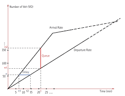
To introduce Little’s law, we first consider some illustrative examples.
(1) At a hospital, on average, 25 new patients are admitted every day. A patient stays an average of four days. What is the average number of busy beds? Denote by $\lambda=25$ the average number of new patients admitted per day, by $W=4$ the average number of days a patient stays at the hospital, and by $L$ the average number of occupied beds. Of course, we have $L=\lambda W=25 \times 4=100$ beds.
(2) A specialty shop sells an average of 100 bottles of a unique Mexican beer per week. On average, the shop has 250 bottles in stock. What is the average number of weeks a bottle is kept in stock? Denote by $\lambda=100$ the average demand per week, by $L=250$ the average number of bottles in stock, and by $W$ the average number of weeks a bottle is kept in stock. The answer is then $W=L / \lambda=250 / 100=2.5$ weeks.

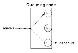
These examples illustrate Little’s law $L=\lambda W$. Little’s law is a sort of law of nature in operations research and applies to almost all queueing systems. This important formula relates the average number of customers in the system (respectively, queue) to a customer’s average sojourn time, that is, the time the customer spends in the system (respectively, waiting time). Let us consider an arbitrary queueing system without specifying the customer’s arrival process, the evolution of the customer service time, or the number of available servers. However, we do assume that the system has an infinite waiting room and that every arriving customer enters and waits to be served. Define the following random variables:
$\begin{aligned} L(t)= & \text { number of customers in the system at time } t \ & \text { (including the customers in service), } \ L_q(t)= & \text { number of customers in the queue at time } t \ & \text { (excluding the customers in service), } \ V_n= & \text { time the } n \text {th customers spends in the system } \ & \text { (including service time), } \ W_n= & \text { time the } n \text {th customer spends waiting in line } \ & \text { (excluding service time). }\end{aligned}$

运筹学代考

数学代写|运筹学作业代写operational research代考|Data Analysis

假设泊松过程似乎是顾客到达的合理模型。如何检验到达数据是否证明使用泊松过程是合理的? 粗略地 说，有两种类型的测试：图形测试和统计测试。图形测试是非正式的，只能给人第一印象。统计测试基 于正式标准。在本节中，我们将简要讨论图解法 $Q-Q$ 图和 Kolmogorov-Smirnov 的统计检验。
在泊松过程中，客户到达间隔时间是具有共同指数分布的独立随机变量。 $\mathrm{A}-Q$ plot 是验证期望数据 来自指数分布是否合理的第一步。更一般地，一个 $Q-Q$ plot 用于获得概率分布族的概念，在其中搜索 适合数据的分布。 $\mathrm{A} Q-Q$ plot 是比数据直方图更好的视觉辅助工具。这尤其适用于数据来自连续分布 的情况：直方图子区间长度的选择会极大地影响直方图的形状。的巨大优势 $Q-Q$ plot 是对于概率分布 的主要系列，没有必要事先知道相关分布的参数。 $\mathrm{A} Q-Q$ 该图显示了根据所提出的理论分布的百分位 数设置的经验分布的百分位数是否大致位于一条直线上。如果 $F(x)$ 是连续概率分布函数，则 $p$ 理论分布 函数的第 th 个百分位数 $F(x)$ 被定义为最小的数 $x_p$ 和
$$
F\left(x_p\right)=p \quad \text { for } 0<p<1
$$
假如说 $F(x)$ 严格递增， $x_p$ 是（谁）给的
$$
x_p=F^{-1}(p)
$$
对于数据的经验分布，百分位数确定如下。假设数据 $X_1, \ldots, X_n$ 来自连续概率分布，将数据排序为
$$
X_{(1)}<X_{(2)}<\cdots<X_{(n)}
$$

数学代写|运筹学作业代写operational research代考|Fundamental Queueing Results

为了介绍利特尔定律，我们首先考虑一些说明性的例子。
(1) 在一家医院，平均每天有 25 名新病人入院。患者平均停留四天。繁忙床位的平均数量是多少? 表示 为 $\lambda=25$ 平均每天入院的新病人数，按 $W=4$ 患者住院的平均天数，以及 $L$ 占用床位的平均数量。当 然，我们有 $L=\lambda W=25 \times 4=100$ 床。
(2) 一家专卖店平均每周销售 100 瓶独特的墨西哥啤酒。该店平均有 250 瓶库存。一瓶酒的平均库存周数 是多少? 表示为 $\lambda=100$ 每周平均需求，由 $L=250$ 库存瓶子的平均数量，以及 $W-$ 瓶酒的平均库存周 数。那么答案就是 $W=L / \lambda=250 / 100=2.5$ 周。
这些例子说明了利特尔定律 $L=\lambda W$. 利特尔定律是运筹学中的一种自然规律，几乎适用于所有的排队 系统。这个重要的公式将系统中客户的平均数量 (分别称为队列) 与客户的平均逗留时间相关联，即客 户在系统中花费的时间 (分别称为等待时间) 。让我们考虑一个任意的排队系统，而不指定客户的到达 过程、客户服务时间的演变或可用服务器的数量。然而，我们确实假设系统有一个无限的等候室，每个 到达的顾客都会进入并等待服务。定义以下随机变量:
$L(t)=$ number of customers in the system at time $t$
(including the customers in ser

统计代写请认准statistics-lab™. statistics-lab™为您的留学生涯保驾护航。

金融工程代写

金融工程是使用数学技术来解决金融问题。金融工程使用计算机科学、统计学、经济学和应用数学领域的工具和知识来解决当前的金融问题，以及设计新的和创新的金融产品。

非参数统计代写

非参数统计指的是一种统计方法，其中不假设数据来自于由少数参数决定的规定模型；这种模型的例子包括正态分布模型和线性回归模型。

广义线性模型代考

广义线性模型（GLM）归属统计学领域，是一种应用灵活的线性回归模型。该模型允许因变量的偏差分布有除了正态分布之外的其它分布。

术语 广义线性模型（GLM）通常是指给定连续和/或分类预测因素的连续响应变量的常规线性回归模型。它包括多元线性回归，以及方差分析和方差分析（仅含固定效应）。

有限元方法代写

有限元方法（FEM）是一种流行的方法，用于数值解决工程和数学建模中出现的微分方程。典型的问题领域包括结构分析、传热、流体流动、质量运输和电磁势等传统领域。

有限元是一种通用的数值方法，用于解决两个或三个空间变量的偏微分方程（即一些边界值问题）。为了解决一个问题，有限元将一个大系统细分为更小、更简单的部分，称为有限元。这是通过在空间维度上的特定空间离散化来实现的，它是通过构建对象的网格来实现的：用于求解的数值域，它有有限数量的点。边界值问题的有限元方法表述最终导致一个代数方程组。该方法在域上对未知函数进行逼近。[1] 然后将模拟这些有限元的简单方程组合成一个更大的方程系统，以模拟整个问题。然后，有限元通过变化微积分使相关的误差函数最小化来逼近一个解决方案。

tatistics-lab作为专业的留学生服务机构，多年来已为美国、英国、加拿大、澳洲等留学热门地的学生提供专业的学术服务，包括但不限于Essay代写，Assignment代写，Dissertation代写，Report代写，小组作业代写，Proposal代写，Paper代写，Presentation代写，计算机作业代写，论文修改和润色，网课代做，exam代考等等。写作范围涵盖高中，本科，研究生等海外留学全阶段，辐射金融，经济学，会计学，审计学，管理学等全球99%专业科目。写作团队既有专业英语母语作者，也有海外名校硕博留学生，每位写作老师都拥有过硬的语言能力，专业的学科背景和学术写作经验。我们承诺100%原创，100%专业，100%准时，100%满意。

随机分析代写

随机微积分是数学的一个分支，对随机过程进行操作。它允许为随机过程的积分定义一个关于随机过程的一致的积分理论。这个领域是由日本数学家伊藤清在第二次世界大战期间创建并开始的。

时间序列分析代写

随机过程，是依赖于参数的一组随机变量的全体，参数通常是时间。 随机变量是随机现象的数量表现，其时间序列是一组按照时间发生先后顺序进行排列的数据点序列。通常一组时间序列的时间间隔为一恒定值（如1秒，5分钟，12小时，7天，1年），因此时间序列可以作为离散时间数据进行分析处理。研究时间序列数据的意义在于现实中，往往需要研究某个事物其随时间发展变化的规律。这就需要通过研究该事物过去发展的历史记录，以得到其自身发展的规律。

回归分析代写

多元回归分析渐进（Multiple Regression Analysis Asymptotics）属于计量经济学领域，主要是一种数学上的统计分析方法，可以分析复杂情况下各影响因素的数学关系，在自然科学、社会和经济学等多个领域内应用广泛。

MATLAB代写

MATLAB 是一种用于技术计算的高性能语言。它将计算、可视化和编程集成在一个易于使用的环境中，其中问题和解决方案以熟悉的数学符号表示。典型用途包括：数学和计算算法开发建模、仿真和原型制作数据分析、探索和可视化科学和工程图形应用程序开发，包括图形用户界面构建MATLAB 是一个交互式系统，其基本数据元素是一个不需要维度的数组。这使您可以解决许多技术计算问题，尤其是那些具有矩阵和向量公式的问题，而只需用 C 或 Fortran 等标量非交互式语言编写程序所需的时间的一小部分。MATLAB 名称代表矩阵实验室。MATLAB 最初的编写目的是提供对由 LINPACK 和 EISPACK 项目开发的矩阵软件的轻松访问，这两个项目共同代表了矩阵计算软件的最新技术。MATLAB 经过多年的发展，得到了许多用户的投入。在大学环境中，它是数学、工程和科学入门和高级课程的标准教学工具。在工业领域，MATLAB 是高效研究、开发和分析的首选工具。MATLAB 具有一系列称为工具箱的特定于应用程序的解决方案。对于大多数 MATLAB 用户来说非常重要，工具箱允许您学习和应用专业技术。工具箱是 MATLAB 函数（M 文件）的综合集合，可扩展 MATLAB 环境以解决特定类别的问题。可用工具箱的领域包括信号处理、控制系统、神经网络、模糊逻辑、小波、仿真等。

R语言代写	问卷设计与分析代写
PYTHON代写	回归分析与线性模型代写
MATLAB代写	方差分析与试验设计代写
STATA代写	机器学习/统计学习代写
SPSS代写	计量经济学代写
EVIEWS代写	时间序列分析代写
EXCEL代写	深度学习代写
SQL代写	各种数据建模与可视化代写

statistics-lab™ 为您的留学生涯保驾护航 在代写运筹学operational research方面已经树立了自己的口碑, 保证靠谱, 高质且原创的统计Statistics代写服务。我们的专家在代写运筹学operational research代写方面经验极为丰富，各种代写运筹学operational research相关的作业也就用不着说。

我们提供的运筹学operational research及其相关学科的代写，服务范围广, 其中包括但不限于:

• Statistical Inference 统计推断
• Statistical Computing 统计计算
• Advanced Probability Theory 高等楖率论
• Advanced Mathematical Statistics 高等数理统计学
• (Generalized) Linear Models 广义线性模型
• Statistical Machine Learning 统计机器学习
• Longitudinal Data Analysis 纵向数据分析
• Foundations of Data Science 数据科学基础

数学代写|运筹学作业代写operational research代考|Balance Equations

In this subsection, we make the following assumption for the Markov chain.

Assumption 7.1. There is a state $r$ that can ultimately be reached from every initial state $i$ with probability 1 , and the expected value of the number of steps needed to return from state $r$ to itself is finite.

This assumption is satisfied in almost every practical application concerning the equilibrium of the Markov chain. For a Markov chain with a finite state space $I$, the assumption is automatically satisfied when the Markov chain has no two disjoint closed sets. Under Assumption 7.1, one can prove that for all $i, j \in I$,
$$
\pi_j=\lim {n \rightarrow \infty} \frac{1}{n} \sum{t=1}^n p_{i j}^{(t)}
$$
is independent of the initial state $i$, and moreover $\sum_{j \in I} \pi_j=1$. Thus, $\pi_j$ is the expected fraction of time $\lim {n \rightarrow \infty} \frac{1}{n} \sum{t=1}^n p_{i j}^{(t)}$ that the process is in state $j$. The fraction $\pi_j$ is related to the mean first passage time to reach state $j$ from state $j$, $m_{j j}$, as
$$
\pi_j=\frac{1}{m_{j j}}
$$
The interpretation of $\lim {n \rightarrow \infty} \frac{1}{n} \sum{t=1}^n p_{i j}^{(t)}$ as the expected fraction of the time that the process is in state $j$ can be extended to the stronger interpretation:
the actual long-run fraction of the time the process is in state $j$ $=\pi_j \quad$ with probability 1
independently of the initial state $X_0=i$. We do not prove this extremely important interpretation, nor the result that $\lim {n \rightarrow \infty} p{i j}^{(n)}$ exists and $\pi_j$ is also given by $\lim {n \rightarrow \infty} p{i j}^{(n)}$ if the Markov chain satisfies Assumption 7.1 and is aperiodic.
Definition 7.5 (Ergodic Markov chain). An irreducible, aperiodic, positive recurrent Markov chain with stationary distribution is called ergodic.

A Markov chain is ergodic if Assumption 7.1 is satisfied and the state space $I$ is a single irreducible set. We prove the weaker interpretation of $\pi_j$ as the expected fraction of time that the process is in state $j$.

数学代写|运筹学作业代写operational research代考|Markov Chains with a Cost Structure

Many practical problems concern Markov chains with a cost or revenue structure. Suppose that every time the Markov chain makes a transition to state $j$, a cost of $c(j)$ is incurred. What is the long-run average cost per unit of time? Intuitively, it should be clear that this cost is equal to $\sum_{j \in I} c(j) \pi_j$ because $\pi_j$ can be interpreted as the average number of transitions to state $j$ per unit of time. To give a mathematical proof that this cost formula is correct, we need a technical assumption in addition to the earlier assumption that there is a state $r$ that is ultimately reached from the initial state $i$ with probability 1 . The additional assumption is that $\sum_{j \in I}|c(j)| \pi_j<$ $\infty$ and that for every initial state $i \in I$, the total cost made until the first return to state $r$ has a finite expected value. This assumption is automatically satisfied if the Markov chain has a finite state space and no two disjoint closed sets. The following main theorem holds.
Theorem 7.5. The actual long-run average cost per unit of time is given by
$$
\lim {n \rightarrow \infty} \frac{1}{n} \sum{t=1}^n c\left(X_t\right)=\sum_{j \in I} c(j) \pi_j \quad \text { with probability } 1
$$
independently of the initial state $X_0=i$.
We do not give the proof of this so-called ergodic theorem. It relies on the famous renewal-reward theorem from the theory of regenerative stochastic processes. The proof moreover shows that the theorem also applies to the case of continuous costs between the state transitions rather than direct costs $c(j)$. If, in the continuous case, we define the cost function $c(j)$ by
$$
c(j)=\mathrm{E}\left[\text { cost between the times } t=n-1 \text { and } t=n \mid X_{n-1}=j\right] \text {, }
$$ then it is also true that the actual long-run average cost per unit of time is equal to $\sum_{j \in I} c(j) \pi_j$ with probability 1. This is an extremely useful observation for real-world applications. In applications, it can also be helpful to interpret certain performance measures as average costs per unit of time.

运筹学代考

数学代写|运筹学作业代写operational research代考|Balance Equations

在本小节中，我们对马尔可夫链做出以下假设。
假设 7.1。有一个状态 $r$ 最终可以从每个初始状态达到 $i$ 概率为 1 ，以及从状态返回所需的步数的期望值 $r$ 对自身是有限的。
几乎所有涉及马尔可夫链平衡的实际应用都满足该假设。对于具有有限状态空间的马尔可夫链 $I$ ，当马尔 可夫链没有两个不相交的闭集时，假设自动满足。在假设 7.1 下，可以证明对于所有 $i, j \in I$ ，
$$
\pi_j=\lim n \rightarrow \infty \frac{1}{n} \sum t=1^n p_{i j}^{(t)}
$$
独立于初始状态 $i$ ，而且 $\sum_{j \in I} \pi_j=1$. 因此， $\pi_j$ 是预期的时间分数 $\lim n \rightarrow \infty \frac{1}{n} \sum t=1^n p_{i j}^{(t)}$ 该过 程处于状态 $j$. 分数 $\pi_j$ 与到达状态的平均首次通过时间有关 $j$ 来自州 $j, m_{j j}$ ， 作为
$$
\pi_j=\frac{1}{m_{j j}}
$$
的解释 $\lim n \rightarrow \infty \frac{1}{n} \sum t=1^n p_{i j}^{(t)}$ 作为进程处于状态的时间的预期分数 $j$ 可以扩展到更强的解释:
过程处于状态的时间的实际长期分数 $j=\pi_j$
与初始状态无关的概率为 $1 X_0=i$. 我们不证明这个极其重要的解释，也不证明那个结果
$\lim n \rightarrow \infty p i j^{(n)}$ 存在并且 $\pi_j$ 也由 $\lim n \rightarrow \infty p i j^{(n)}$ 如果马尔可夫链满足假设 7.1 并且是非周期性 的。
定义 7.5 (遍历马尔可夫链) 。具有平稳分布的不可约、非周期、正循环马尔可夫链称为遍历。
如果满足假设 7.1 并且状态空间，则马尔可夫链是遍历的 $I$ 是单个不可约集。我们证明了较弱的解释 $\pi_j$ 作 为进程处于状态的预期时间分数 $j$.

数学代写|运筹学作业代写operational research代考|Markov Chains with a Cost Structure

许多实际问题都与具有成本或收入结构的马尔可夫链有关。假设每次马尔可夫链转换到状态 $j$, 的成本 $c(j)$ 被招致。单位时间的长期平均成本是多少? 直觉上，应该清楚这个成本等于 $\sum_{j \in I} c(j) \pi_j$ 因为 $\pi_j$ 可以解 释为状态转换的平均次数 $j$ 每单位时间。为了给出这个成本公式正确的数学证明，除了早先假设存在状态 之外，我们还需要一个技术假设 $r$ 从初始状态最终达到 $i$ 概率为 1 。额外的假设是 $\sum_{j \in I}|c(j)| \pi_j<\infty$ 并 且对于每个初始状态 $i \in I$ ，直到第一次返回状态的总成本 $r$ 有一个有限的期望值。如果马尔可夫链具有有 限状态空间并且没有两个不相交的闭集，则自动满足此假设。下面的主要定理成立。
定理 7.5。每单位时间的实际长期平均成本为
$$
\lim n \rightarrow \infty \frac{1}{n} \sum t=1^n c\left(X_t\right)=\sum_{j \in I} c(j) \pi_j \quad \text { with probability } 1
$$
独立于初始状态 $X_0=i$.
我们不给出这个所谓的遍历定理的证明。它依赖于再生随机过程理论中著名的更新奖励定理。证明还表 明，该定理也适用于状态转换之间的连续成本而不是直接成本的情况 $c(j)$. 如果在连续情况下，我们定义 成本函数 $c(j)$ 经过
$$
c(j)=\mathrm{E}\left[\text { cost between the times } t=n-1 \text { and } t=n \mid X_{n-1}=j\right],
$$
那么每单位时间的实际长期平均成本也等于 $\sum_{j \in I} c(j) \pi_j$ 概率为 1 。这对于实际应用来说是一个非常有用 的观察结果。在应用程序中，将某些性能度量解释为每单位时间的平均成本也很有帮助。

统计代写请认准statistics-lab™. statistics-lab™为您的留学生涯保驾护航。

金融工程代写

金融工程是使用数学技术来解决金融问题。金融工程使用计算机科学、统计学、经济学和应用数学领域的工具和知识来解决当前的金融问题，以及设计新的和创新的金融产品。

非参数统计代写

非参数统计指的是一种统计方法，其中不假设数据来自于由少数参数决定的规定模型；这种模型的例子包括正态分布模型和线性回归模型。

广义线性模型代考

广义线性模型（GLM）归属统计学领域，是一种应用灵活的线性回归模型。该模型允许因变量的偏差分布有除了正态分布之外的其它分布。

术语 广义线性模型（GLM）通常是指给定连续和/或分类预测因素的连续响应变量的常规线性回归模型。它包括多元线性回归，以及方差分析和方差分析（仅含固定效应）。

有限元方法代写

有限元方法（FEM）是一种流行的方法，用于数值解决工程和数学建模中出现的微分方程。典型的问题领域包括结构分析、传热、流体流动、质量运输和电磁势等传统领域。

有限元是一种通用的数值方法，用于解决两个或三个空间变量的偏微分方程（即一些边界值问题）。为了解决一个问题，有限元将一个大系统细分为更小、更简单的部分，称为有限元。这是通过在空间维度上的特定空间离散化来实现的，它是通过构建对象的网格来实现的：用于求解的数值域，它有有限数量的点。边界值问题的有限元方法表述最终导致一个代数方程组。该方法在域上对未知函数进行逼近。[1] 然后将模拟这些有限元的简单方程组合成一个更大的方程系统，以模拟整个问题。然后，有限元通过变化微积分使相关的误差函数最小化来逼近一个解决方案。

tatistics-lab作为专业的留学生服务机构，多年来已为美国、英国、加拿大、澳洲等留学热门地的学生提供专业的学术服务，包括但不限于Essay代写，Assignment代写，Dissertation代写，Report代写，小组作业代写，Proposal代写，Paper代写，Presentation代写，计算机作业代写，论文修改和润色，网课代做，exam代考等等。写作范围涵盖高中，本科，研究生等海外留学全阶段，辐射金融，经济学，会计学，审计学，管理学等全球99%专业科目。写作团队既有专业英语母语作者，也有海外名校硕博留学生，每位写作老师都拥有过硬的语言能力，专业的学科背景和学术写作经验。我们承诺100%原创，100%专业，100%准时，100%满意。

随机分析代写

随机微积分是数学的一个分支，对随机过程进行操作。它允许为随机过程的积分定义一个关于随机过程的一致的积分理论。这个领域是由日本数学家伊藤清在第二次世界大战期间创建并开始的。

时间序列分析代写

随机过程，是依赖于参数的一组随机变量的全体，参数通常是时间。 随机变量是随机现象的数量表现，其时间序列是一组按照时间发生先后顺序进行排列的数据点序列。通常一组时间序列的时间间隔为一恒定值（如1秒，5分钟，12小时，7天，1年），因此时间序列可以作为离散时间数据进行分析处理。研究时间序列数据的意义在于现实中，往往需要研究某个事物其随时间发展变化的规律。这就需要通过研究该事物过去发展的历史记录，以得到其自身发展的规律。

回归分析代写

多元回归分析渐进（Multiple Regression Analysis Asymptotics）属于计量经济学领域，主要是一种数学上的统计分析方法，可以分析复杂情况下各影响因素的数学关系，在自然科学、社会和经济学等多个领域内应用广泛。

MATLAB代写

MATLAB 是一种用于技术计算的高性能语言。它将计算、可视化和编程集成在一个易于使用的环境中，其中问题和解决方案以熟悉的数学符号表示。典型用途包括：数学和计算算法开发建模、仿真和原型制作数据分析、探索和可视化科学和工程图形应用程序开发，包括图形用户界面构建MATLAB 是一个交互式系统，其基本数据元素是一个不需要维度的数组。这使您可以解决许多技术计算问题，尤其是那些具有矩阵和向量公式的问题，而只需用 C 或 Fortran 等标量非交互式语言编写程序所需的时间的一小部分。MATLAB 名称代表矩阵实验室。MATLAB 最初的编写目的是提供对由 LINPACK 和 EISPACK 项目开发的矩阵软件的轻松访问，这两个项目共同代表了矩阵计算软件的最新技术。MATLAB 经过多年的发展，得到了许多用户的投入。在大学环境中，它是数学、工程和科学入门和高级课程的标准教学工具。在工业领域，MATLAB 是高效研究、开发和分析的首选工具。MATLAB 具有一系列称为工具箱的特定于应用程序的解决方案。对于大多数 MATLAB 用户来说非常重要，工具箱允许您学习和应用专业技术。工具箱是 MATLAB 函数（M 文件）的综合集合，可扩展 MATLAB 环境以解决特定类别的问题。可用工具箱的领域包括信号处理、控制系统、神经网络、模糊逻辑、小波、仿真等。

R语言代写	问卷设计与分析代写
PYTHON代写	回归分析与线性模型代写
MATLAB代写	方差分析与试验设计代写
STATA代写	机器学习/统计学习代写
SPSS代写	计量经济学代写
EVIEWS代写	时间序列分析代写
EXCEL代写	深度学习代写
SQL代写	各种数据建模与可视化代写

statistics-lab™ 为您的留学生涯保驾护航 在代写运筹学operational research方面已经树立了自己的口碑, 保证靠谱, 高质且原创的统计Statistics代写服务。我们的专家在代写运筹学operational research代写方面经验极为丰富，各种代写运筹学operational research相关的作业也就用不着说。

我们提供的运筹学operational research及其相关学科的代写，服务范围广, 其中包括但不限于:

• Statistical Inference 统计推断
• Statistical Computing 统计计算
• Advanced Probability Theory 高等楖率论
• Advanced Mathematical Statistics 高等数理统计学
• (Generalized) Linear Models 广义线性模型
• Statistical Machine Learning 统计机器学习
• Longitudinal Data Analysis 纵向数据分析
• Foundations of Data Science 数据科学基础

数学代写|运筹学作业代写operational research代考|Equilibrium and Stationary Probabilities

We observed in Example 7.6 that $\lim {n \rightarrow \infty} p{i j}^{(n)}$ converged to a limit that does not depend on the initial state $i$. Now suppose that this limit exists for all $i, j \in I$ and is independent of the initial state $i$, and denote the limit by $\pi_j$, i.e.,
$$
\pi_j=\lim {n \rightarrow \infty} p{i j}^{(n)} \quad \text { for all } i, j \in I
$$
and moreover assume that the state space $I$ is finite, then
$$
\pi_j=\sum_{k \in I} \pi_k p_{k j} \quad \text { for all } j \in I .
$$
This immediately follows by taking $n \rightarrow \infty$ in $p_{i j}^{(n+1)}=\sum_{k \in I} p_{i k}^{(n)} p_{k j}$, the ChapmanKolmogorov equations (7.2) for $m=1$, and reversing the order of the limit and sum. This brings us to calling the $\left{\pi_j\right}$ the equilibrium distribution. We may also consider a stationary distribution.

Definition 7.2. A probability distribution $\left{\eta_j, j \in I\right}$ is called a stationary distribution of the Markov chain if
$$
\eta_j=\sum_{k \in I} \eta_k p_{k j} \quad \text { for all } j \in I .
$$
The reason behind this name is as follows. Suppose that the initial state $X_0$ is determined by drawing lots with probabilities
$$
\mathbb{P}\left(X_0=j\right)=\eta_j \quad \text { for all } j \in I
$$

From the point of view of an outsider who has this as only information and does not know which state has emerged from the draw, the state of the process at any future time $n$ will be $j$ with probability
$$
\mathbb{P}\left(X_n=j\right)=\eta_j \quad \text { for all } j \in I \text {. }
$$
It is easy to show this using induction. Suppose that for $k=0, \ldots, m$, we know that $\mathbb{P}\left(X_k=j\right)=\eta_j$ for all $j$; then
$$
\begin{aligned}
\mathbb{P}\left(X_{m+1}=j\right) & =\sum_{k \in I} \mathbb{P}\left(X_{m+1}=j \mid X_m=k\right) \mathbb{P}\left(X_m=k\right) \
& =\sum_{k \in I} \mathbb{P}\left(X_m=k\right) p_{k j}=\sum_{k \in I} \eta_k p_{k j}=\eta_j
\end{aligned}
$$
The next sections consider the limiting behavior and investigate in more detail when the equilibrium distribution $\left{\pi_j\right}$ from $(7.4)$ is a stationary distribution.

数学代写|运筹学作业代写operational research代考|Limiting Behavior

Natural questions are whether the $n$-step transition probabilities $p_{i j}^{(n)}$ always have a limit as $n \rightarrow \infty$ and, if so, whether the limit is also independent of the initial state $i$. The answer to these questions is not always “yes.” The easiest way to see this is through counterexamples. Suppose that a Markov chain has state space $I={1,2}$ with one-step transition probabilities $p_{12}=p_{21}=1$ and $p_{11}=p_{22}=0$. Then $p_{i j}^{(n)}$ alternates between 0 and 1 for $n=1,2, \ldots$ and therefore has no limit as $n \rightarrow \infty$. The reason this limit does not exist lies in the periodicity of the state transitions.
Definition 7.3 (Periodic Markov chain). A Markov chain is called periodic if there exist at least two disjoint subsets $R_1, \ldots, R_d$ of the state space such that a state in $R_k$ always transitions to a state in $R_{k+1}$ for $k=1, \ldots, d$ (with $R_{d+1}=R_1$ ). If this is not the case, then the Markov chain is called aperiodic.

The random walk of Example 7.7 may return to state 0 after an even number of steps, only. Here $R_1$ contains the even numbers and $R_2$ the odd numbers.

Even if the limit of the $p_{i j}^{(n)}$ exists, it is not necessarily independent of the initial state. Consider the Markov chain with state space $I={1,2}$ and one-step transition probabilities $p_{11}=p_{22}=1$ and $p_{12}=p_{21}=0$. Then $p_{11}^{(n)}=1$ and $p_{21}^{(n)}=0$ for all $n \geq 1$, so that $\lim {n \rightarrow \infty} p{i 1}^{(n)}$ depends on the initial state $i$. This dependence occurs when the Markov chain has two or more disjoint closed sets. Recall that a set $I^{\prime} \subset I$ is closed if $p_{i j}=0$ for $i \in I^{\prime}$ and $j \notin I^{\prime}$. The set $I^{\prime}$ is an irreducible set if it is closed and all its states communicate. Two irreducible sets must be disjoint (verify!). The state space may therefore be decomposed into disjoint irreducible sets $I_1, I_2, \ldots$, and a non-irreducible set $I^*$.

Definition 7.4 (Irreducible Markov chain). A Markov chain is called irreducible if every state $k$ is reachable from every other state $j$; that is, for all $j, k \in I$, there is an $n \geq 1$ such that $p_{j k}^{(n)}>0$.

A Markov chain is irreducible if its state space is an irreducible set.
The examples above show that conditions must be imposed on the Markov chain when the limiting behavior of the Markov chain is studied. For a Markov chain with a finite state space $I$, one can show that $\lim {n \rightarrow \infty} p{i j}^{(n)}$ exists for all $i, j$ if the Markov chain is aperiodic, where the limit is moreover independent of the initial state $i$ if the Markov chain does not contain two or more disjoint closed sets. In the case of Example 7.6, these conditions hold and therefore, as $n \rightarrow \infty$, the matrix $\mathbf{P}^n$ converges to a limiting matrix in which all rows are the same. In applications, however, the aperiodicity does not always hold. For instance, in Example 7.2 , the Markov chain is periodic with period 2 (from an even state, the process always goes to an odd state, and vice versa). In applications of Markov chains in operations research, whether or not a Markov chain is aperiodic is rarely relevant. In these applications, the important concept is that of the so-called Cesàro limit ${ }^4$
$$
\lim {n \rightarrow \infty} \frac{1}{n} \sum{t=1}^n p_{i j}^{(t)}
$$

运筹学代考

数学代写|运筹学作业代写operational research代考|Equilibrium and Stationary Probabilities

我们在例 7.6 中观察到 $\lim n \rightarrow \infty p i j^{(n)}$ 收敛到一个不依赖于初始状态的极限 $i$. 现在假设这个限制对所 有人都存在 $i, j \in I$ 并且独立于初始状态 $i$ ，并表示极限 $\pi_j$ ，那是，
$$
\pi_j=\lim n \rightarrow \infty p i j^{(n)} \quad \text { for all } i, j \in I
$$
而且假设状态空间 $I$ 是有限的，那么
$$
\pi_j=\sum_{k \in I} \pi_k p_{k j} \quad \text { for all } j \in I
$$
这紧随其后 $n \rightarrow \infty$ 在 $p_{i j}^{(n+1)}=\sum_{k \in I} p_{i k}^{(n)} p_{k j}$, ChapmanKolmogorov 方程 (7.2) 为 $m=1$ ，并颠倒极
定义 7.2。概率分布 《eft{teta_j, j \in Iright} 称为马尔可夫链的平稳分布，如果
$$
\eta_j=\sum_{k \in I} \eta_k p_{k j} \quad \text { for all } j \in I
$$
这个名字背后的原因如下。假设初始状态 $X_0$ 由抽签决定
$$
\mathbb{P}\left(X_0=j\right)=\eta_j \quad \text { for all } j \in I
$$
从仅将此作为信息并且不知道从平局中出现哪种状态的局外人的角度来看，末来任何时候的过程状态 $n$ 将 $j$ 有概率
$$
\mathbb{P}\left(X_n=j\right)=\eta_j \quad \text { for all } j \in I .
$$
使用归纳法很容易证明这一点。假设对于 $k=0, \ldots, m$ ，我们知道 $\mathbb{P}\left(X_k=j\right)=\eta_j$ 对全部 $j$; 然后
$$
\mathbb{P}\left(X_{m+1}=j\right)=\sum_{k \in I} \mathbb{P}\left(X_{m+1}=j \mid X_m=k\right) \mathbb{P}\left(X_m=k\right) \quad=\sum_{k \in I} \mathbb{P}\left(X_m=k\right) p_{k j}=\sum_{k \in I}
$$
下一节考虑限制行为，并在平衡分布时更详细地研究 $\mid$ 左{ipi_j右} 从 (7.4)是平稳分布。

数学代写|运筹学作业代写operational research代考|Limiting Behavior

自然的问题是 $n$-步转移概率 $p_{i j}^{(n)}$ 总是有一个限制 $n \rightarrow \infty$ 并且，如果是，极限是否也独立于初始状态 $i$. 这 些问题的答案并不总是“是”。看到这一点的最简单方法是通过反例。假设马尔可夫链有状态空间 $I=1,2$ 一步转移概率 $p_{12}=p_{21}=1$ 和 $p_{11}=p_{22}=0$. 然后 $p_{i j}^{(n)}$ 在 0 和 1 之间交替 $n=1,2, \ldots$. 因此没有限 制 $n \rightarrow \infty$. 这个限制不存在的原因在于状态转换的周期性。
定义 7.3 (周期马尔可夫链) 。如果存在至少两个不相交的子集，则马尔可夫链称为周期性的 $R_1, \ldots, R_d$ 状态空间使得状态在 $R_k$ 总是转换到一个状态 $R_{k+1}$ 为了 $k=1, \ldots, d$ (和 $R_{d+1}=R_1$ ). 如 果不是这种情况，则称马尔可夫链是非周期性的。
示例 7.7 的随机游走可能仅在偶数步后返回到状态 0 。这里 $R_1$ 包含偶数和 $R_2$ 奇数。
即使限制了 $p_{i j}^{(n)}$ 存在，它不一定独立于初始状态。考虑具有状态空间的马尔可夫链 $I=1,2$ 和一步转移概 率 $p_{11}=p_{22}=1$ 和 $p_{12}=p_{21}=0$. 然后 $p_{11}^{(n)}=1$ 和 $p_{21}^{(n)}=0$ 对全部 $n \geq 1$ ，以便
$\lim n \rightarrow \infty p i 1^{(n)}$ 取决于初始状态 $i$. 当马尔可夫链有两个或多个不相交的闭集时，就会出现这种依赖 性。回想一下，一组 $I^{\prime} \subset I$ 关闭如果 $p_{i j}=0$ 为了 $i \in I^{\prime}$ 和 $j \notin I^{\prime}$. 庡装 $I^{\prime}$ 是一个不可约集，如果它是封 闭的并且它的所有状态都通信。两个不可约集必须不相交 (验证!)）。因此，状态空间可以分解为不相交 的不可约集 $I_1, I_2, \ldots$, 和一个不可约集 $I^*$.
定义 7.4 (不可约马尔可夫链) 。如果每个状态 $k$ 可以从其他所有州到达 $j$; 也就是说，对于所有 $j, k \in I$ 有一个 $n \geq 1$ 这样 $p_{j k}^{(n)}>0$.
如果状态空间是不可约集，则马尔可夫链是不可约的。
上面的例子表明，在研究马尔可夫链的极限行为时，必须对马尔可夫链施加条件。对于具有有限状态空间 的马尔可夫链 $I$, 可以证明 $\lim n \rightarrow \infty p i j^{(n)}$ 存在于所有人 $i, j$ 如果马尔可夫链是非周期性的，并且极限 独立于初始状态 $i$ 如果马尔可夫链不包含两个或多个不相交的闭集。在示例 7.6 的情况下，这些条件成 立，因此， $n \rightarrow \infty$ ，矩阵 $\mathbf{P}^n$ 收敛到一个限制矩阵，其中所有行都相同。然而，在应用中，非周期性并 不总是成立。例如，在示例 7.2 中，马尔可夫链是周期性的，周期为 2 (从偶数状态，过程总是进入奇数 状态，反之亦然) 。在马尔可夫链在运筹学中的应用中，马尔可夫链是否非周期性几乎无关紧要。在这些 应用中，重要的概念是所谓的切萨罗极限 4
$$
\lim n \rightarrow \infty \frac{1}{n} \sum t=1^n p_{i j}^{(t)}
$$

统计代写请认准statistics-lab™. statistics-lab™为您的留学生涯保驾护航。

金融工程代写

金融工程是使用数学技术来解决金融问题。金融工程使用计算机科学、统计学、经济学和应用数学领域的工具和知识来解决当前的金融问题，以及设计新的和创新的金融产品。

非参数统计代写

非参数统计指的是一种统计方法，其中不假设数据来自于由少数参数决定的规定模型；这种模型的例子包括正态分布模型和线性回归模型。

广义线性模型代考

广义线性模型（GLM）归属统计学领域，是一种应用灵活的线性回归模型。该模型允许因变量的偏差分布有除了正态分布之外的其它分布。

术语 广义线性模型（GLM）通常是指给定连续和/或分类预测因素的连续响应变量的常规线性回归模型。它包括多元线性回归，以及方差分析和方差分析（仅含固定效应）。

有限元方法代写

有限元方法（FEM）是一种流行的方法，用于数值解决工程和数学建模中出现的微分方程。典型的问题领域包括结构分析、传热、流体流动、质量运输和电磁势等传统领域。

有限元是一种通用的数值方法，用于解决两个或三个空间变量的偏微分方程（即一些边界值问题）。为了解决一个问题，有限元将一个大系统细分为更小、更简单的部分，称为有限元。这是通过在空间维度上的特定空间离散化来实现的，它是通过构建对象的网格来实现的：用于求解的数值域，它有有限数量的点。边界值问题的有限元方法表述最终导致一个代数方程组。该方法在域上对未知函数进行逼近。[1] 然后将模拟这些有限元的简单方程组合成一个更大的方程系统，以模拟整个问题。然后，有限元通过变化微积分使相关的误差函数最小化来逼近一个解决方案。

tatistics-lab作为专业的留学生服务机构，多年来已为美国、英国、加拿大、澳洲等留学热门地的学生提供专业的学术服务，包括但不限于Essay代写，Assignment代写，Dissertation代写，Report代写，小组作业代写，Proposal代写，Paper代写，Presentation代写，计算机作业代写，论文修改和润色，网课代做，exam代考等等。写作范围涵盖高中，本科，研究生等海外留学全阶段，辐射金融，经济学，会计学，审计学，管理学等全球99%专业科目。写作团队既有专业英语母语作者，也有海外名校硕博留学生，每位写作老师都拥有过硬的语言能力，专业的学科背景和学术写作经验。我们承诺100%原创，100%专业，100%准时，100%满意。

随机分析代写

随机微积分是数学的一个分支，对随机过程进行操作。它允许为随机过程的积分定义一个关于随机过程的一致的积分理论。这个领域是由日本数学家伊藤清在第二次世界大战期间创建并开始的。

时间序列分析代写

随机过程，是依赖于参数的一组随机变量的全体，参数通常是时间。 随机变量是随机现象的数量表现，其时间序列是一组按照时间发生先后顺序进行排列的数据点序列。通常一组时间序列的时间间隔为一恒定值（如1秒，5分钟，12小时，7天，1年），因此时间序列可以作为离散时间数据进行分析处理。研究时间序列数据的意义在于现实中，往往需要研究某个事物其随时间发展变化的规律。这就需要通过研究该事物过去发展的历史记录，以得到其自身发展的规律。

回归分析代写

多元回归分析渐进（Multiple Regression Analysis Asymptotics）属于计量经济学领域，主要是一种数学上的统计分析方法，可以分析复杂情况下各影响因素的数学关系，在自然科学、社会和经济学等多个领域内应用广泛。

MATLAB代写

MATLAB 是一种用于技术计算的高性能语言。它将计算、可视化和编程集成在一个易于使用的环境中，其中问题和解决方案以熟悉的数学符号表示。典型用途包括：数学和计算算法开发建模、仿真和原型制作数据分析、探索和可视化科学和工程图形应用程序开发，包括图形用户界面构建MATLAB 是一个交互式系统，其基本数据元素是一个不需要维度的数组。这使您可以解决许多技术计算问题，尤其是那些具有矩阵和向量公式的问题，而只需用 C 或 Fortran 等标量非交互式语言编写程序所需的时间的一小部分。MATLAB 名称代表矩阵实验室。MATLAB 最初的编写目的是提供对由 LINPACK 和 EISPACK 项目开发的矩阵软件的轻松访问，这两个项目共同代表了矩阵计算软件的最新技术。MATLAB 经过多年的发展，得到了许多用户的投入。在大学环境中，它是数学、工程和科学入门和高级课程的标准教学工具。在工业领域，MATLAB 是高效研究、开发和分析的首选工具。MATLAB 具有一系列称为工具箱的特定于应用程序的解决方案。对于大多数 MATLAB 用户来说非常重要，工具箱允许您学习和应用专业技术。工具箱是 MATLAB 函数（M 文件）的综合集合，可扩展 MATLAB 环境以解决特定类别的问题。可用工具箱的领域包括信号处理、控制系统、神经网络、模糊逻辑、小波、仿真等。

R语言代写	问卷设计与分析代写
PYTHON代写	回归分析与线性模型代写
MATLAB代写	方差分析与试验设计代写
STATA代写	机器学习/统计学习代写
SPSS代写	计量经济学代写
EVIEWS代写	时间序列分析代写
EXCEL代写	深度学习代写
SQL代写	各种数据建模与可视化代写

statistics-lab™ 为您的留学生涯保驾护航 在代写运筹学operational research方面已经树立了自己的口碑, 保证靠谱, 高质且原创的统计Statistics代写服务。我们的专家在代写运筹学operational research代写方面经验极为丰富，各种代写运筹学operational research相关的作业也就用不着说。

我们提供的运筹学operational research及其相关学科的代写，服务范围广, 其中包括但不限于:

• Statistical Inference 统计推断
• Statistical Computing 统计计算
• Advanced Probability Theory 高等楖率论
• Advanced Mathematical Statistics 高等数理统计学
• (Generalized) Linear Models 广义线性模型
• Statistical Machine Learning 统计机器学习
• Longitudinal Data Analysis 纵向数据分析
• Foundations of Data Science 数据科学基础

数学代写|运筹学作业代写operational research代考|The EPQ Production Model

In the EOQ inventory model from Section 6.1 .1 , it is assumed that the entire replenishment order is received at the same time. This assumption is unrealistic in situations where the goods are not ordered externally but produced internally. The EPQ production model assumes that the good is produced at a rate of $p$ units per unit of time. The demand for the product is deterministic and equal to $D$ units per unit of time. By assumption, no shortage may occur. A production run can be started at any time. The cost of a production run of size $Q$ is $K+v Q$, where $K>0$ is the fixed setup cost and $v$ is the variable production cost per unit of product. The holding cost per unit of product per unit of time is $v r$, where $r$ is an interest factor. In the case of a fixed size $Q$ for each production run, the evolution of the inventory level is shown in Figure 6.3.

During a production run, the inventory level increases continuously by $p-D$ per unit of time. When the production run is complete, the inventory level is therefore $(p-D) \frac{Q}{p}$, after which it decreases to zero at a rate of $D$ per unit of time. The total holding cost in a production run is therefore $v r$ times the area of the triangle in Figure 6.3 (a production cycle is the time interval between the starting times of two consecutive production runs). This area is equal to $\frac{1}{2}(p-d) \frac{Q}{p} \times \frac{Q}{D}$. Combining this with the fact that the number of production cycles per unit of time is equal to $\frac{D}{Q}$ gives the following formula for the total cost per unit of time:
$$
\begin{aligned}
T C(Q) & =\frac{D}{Q}\left[\frac{1}{2} v r(p-d) \frac{Q}{p} \times \frac{Q}{D}+K+v Q\right] \
& =\frac{1}{2} \frac{v r Q(p-d)}{p}+\frac{K D}{Q}+v D .
\end{aligned}
$$
If we set the derivative of the function $T C(Q)$ equal to zero, we find that the optimal size $Q^$ of a production run is $$ Q^=\sqrt{\frac{2 K D p}{v r(p-D)}} .
$$
The EOQ formula has therefore been corrected with the factor $\sqrt{p /(p-D)}$. This factor goes to 1 when the production rate $p$ becomes very high. As in the EOQ model from Section 6.1.1, a small deviation from the optimal production size $Q^*$ has little influence on the total cost per unit of time.

数学代写|运筹学作业代写operational research代考|The Silver-Meal Heuristic

In many real-world lot sizing problems, the demand is not constant but varies over time. A typical example is the situation of contractual delivery, where a contract requires specific quantities of a given product to be delivered to the customer at agreed times.
The assumptions of the dynamic inventory model are as follows:

• The stock of a product can only be replenished by production at the beginning of the given periods $j=1, \ldots, N$.
• For every period $j$, the demand $D_j$ is known. This demand must be met within that period. No ordering beforehand or back-ordering is allowed.
• A stock replenishment in period $j$ is available for the demand in that period and for subsequent periods.
• There is no restriction on the size of a stock replenishment, and sufficient storage space is available.
• The variable production cost of $v$ per unit does not depend on the quantity that is produced.
• The influenceable costs are the fixed production cost (setup cost) and the linear holding cost. A fixed cost of $K>0$ is incurred for each stock replenishment. The holding cost in each period is $h>0$ per unit of stock present at the end of the period, where $h$ is usually given by $h=v \times r$ with $r$ an interest factor for the capital invested in inventory.

运筹学代考

数学代写|运筹学作业代写operational research代考|The EPQ Production Model

在第 6.1.1 节的 EOQ 库存模型中，假设同时收到整个补货订单。在货物不是从外部订购而是在内部生产 的情况下，这种假设是不现实的。EPQ 生产模型假设商品的生产率为 $p$ 每单位时间的单位。对产品的需求 是确定的并且等于 $D$ 每单位时间的单位。根据假设，不会发生短缺。可以随时开始生产运行。一次生产的 成本 $Q$ 是 $K+v Q$ ，在哪里 $K>0$ 是固定的设置成本和 $v$ 是每单位产品的可变生产成本。单位时间单位 产品的持有成本为 $v r$ ，在哪里 $r$ 是兴趣因素。在固定尺寸的情况下 $Q$ 对于每个生产运行，库存水平的演变 如图 6.3 所示。
在生产运行期间，库存水平连续增加 $p-D$ 每单位时间。因此，当生产运行完成时，库存水平为 $(p-D) \frac{Q}{p}$ ，之后它以 $D$ 每单位时间。因此，生产运行中的总持有成本为 $v r$ 乘以图 6.3 中三角形的面积 (一个生产周期是两个连续生产运行的开始时间之间的时间间隔）。这个面积等于 $\frac{1}{2}(p-d) \frac{Q}{p} \times \frac{Q}{D}$. 结 合每单位时间的生产周期数等于 $\frac{D}{Q}$ 对于每单位时间的总成本，给出以下公式:
$$
T C(Q)=\frac{D}{Q}\left[\frac{1}{2} v r(p-d) \frac{Q}{p} \times \frac{Q}{D}+K+v Q\right] \quad=\frac{1}{2} \frac{v r Q(p-d)}{p}+\frac{K D}{Q}+v D
$$
如果我们设置函数的导数 $T C(Q)$ 等于零，我们发现最佳尺寸问^生产运行是
$$
Q^{=} \sqrt{\frac{2 K D p}{v r(p-D)}}
$$
因此，EOQ 公式已使用以下因素进行了修正 $\sqrt{p /(p-D)}$. 当生产率时，这个因素变为 $1 p$ 变得很高。与 第 6.1.1 节的 EOQ 模型一样，与最佳生产规模的小偏差 $Q^*$ 对单位时间内的总成本影响不大。

数学代写|运筹学作业代写operational research代考|The Silver-Meal Heuristic

在许多现实世界的批量大小问题中，需求不是恒定的，而是随时间变化的。一个典型的例子是合同交付的 情况，其中合同要求在约定的时间将特定数量的给定产品交付给客户。 动态库存模型的假设如下:

• 产品的库存只能在给定期间的开始时通过生产来补充 $j=1, \ldots, N$.
• 对于每个时期 $j$ ，需求 $D_j$ 众所周知。该需求必须在该期限内得到满足。不允许提前订购或延迟订 购。
• 期间进货 $j$ 可用于该期间和后续期间的需求。
• 无补货规模限制，有充足的仓储空间。
• 可变生产成本 $v$ 每单位不取决于生产的数量。
• 影响成本是固定生产成本 (设置成本) 和线性持有成本。固定成本 $K>0$ 每次补货都会产生费用。 各期持有成本为 $h>0$ 期末存在的每单位存货，其中 $h$ 通常由 $h=v \times r$ 和 $r$ 投资于存货的资本的利 息因素。

统计代写请认准statistics-lab™. statistics-lab™为您的留学生涯保驾护航。

金融工程代写

金融工程是使用数学技术来解决金融问题。金融工程使用计算机科学、统计学、经济学和应用数学领域的工具和知识来解决当前的金融问题，以及设计新的和创新的金融产品。

非参数统计代写

非参数统计指的是一种统计方法，其中不假设数据来自于由少数参数决定的规定模型；这种模型的例子包括正态分布模型和线性回归模型。

广义线性模型代考

广义线性模型（GLM）归属统计学领域，是一种应用灵活的线性回归模型。该模型允许因变量的偏差分布有除了正态分布之外的其它分布。

术语 广义线性模型（GLM）通常是指给定连续和/或分类预测因素的连续响应变量的常规线性回归模型。它包括多元线性回归，以及方差分析和方差分析（仅含固定效应）。

有限元方法代写

有限元方法（FEM）是一种流行的方法，用于数值解决工程和数学建模中出现的微分方程。典型的问题领域包括结构分析、传热、流体流动、质量运输和电磁势等传统领域。

有限元是一种通用的数值方法，用于解决两个或三个空间变量的偏微分方程（即一些边界值问题）。为了解决一个问题，有限元将一个大系统细分为更小、更简单的部分，称为有限元。这是通过在空间维度上的特定空间离散化来实现的，它是通过构建对象的网格来实现的：用于求解的数值域，它有有限数量的点。边界值问题的有限元方法表述最终导致一个代数方程组。该方法在域上对未知函数进行逼近。[1] 然后将模拟这些有限元的简单方程组合成一个更大的方程系统，以模拟整个问题。然后，有限元通过变化微积分使相关的误差函数最小化来逼近一个解决方案。

tatistics-lab作为专业的留学生服务机构，多年来已为美国、英国、加拿大、澳洲等留学热门地的学生提供专业的学术服务，包括但不限于Essay代写，Assignment代写，Dissertation代写，Report代写，小组作业代写，Proposal代写，Paper代写，Presentation代写，计算机作业代写，论文修改和润色，网课代做，exam代考等等。写作范围涵盖高中，本科，研究生等海外留学全阶段，辐射金融，经济学，会计学，审计学，管理学等全球99%专业科目。写作团队既有专业英语母语作者，也有海外名校硕博留学生，每位写作老师都拥有过硬的语言能力，专业的学科背景和学术写作经验。我们承诺100%原创，100%专业，100%准时，100%满意。

随机分析代写

随机微积分是数学的一个分支，对随机过程进行操作。它允许为随机过程的积分定义一个关于随机过程的一致的积分理论。这个领域是由日本数学家伊藤清在第二次世界大战期间创建并开始的。

时间序列分析代写

随机过程，是依赖于参数的一组随机变量的全体，参数通常是时间。 随机变量是随机现象的数量表现，其时间序列是一组按照时间发生先后顺序进行排列的数据点序列。通常一组时间序列的时间间隔为一恒定值（如1秒，5分钟，12小时，7天，1年），因此时间序列可以作为离散时间数据进行分析处理。研究时间序列数据的意义在于现实中，往往需要研究某个事物其随时间发展变化的规律。这就需要通过研究该事物过去发展的历史记录，以得到其自身发展的规律。

回归分析代写

多元回归分析渐进（Multiple Regression Analysis Asymptotics）属于计量经济学领域，主要是一种数学上的统计分析方法，可以分析复杂情况下各影响因素的数学关系，在自然科学、社会和经济学等多个领域内应用广泛。

MATLAB代写

MATLAB 是一种用于技术计算的高性能语言。它将计算、可视化和编程集成在一个易于使用的环境中，其中问题和解决方案以熟悉的数学符号表示。典型用途包括：数学和计算算法开发建模、仿真和原型制作数据分析、探索和可视化科学和工程图形应用程序开发，包括图形用户界面构建MATLAB 是一个交互式系统，其基本数据元素是一个不需要维度的数组。这使您可以解决许多技术计算问题，尤其是那些具有矩阵和向量公式的问题，而只需用 C 或 Fortran 等标量非交互式语言编写程序所需的时间的一小部分。MATLAB 名称代表矩阵实验室。MATLAB 最初的编写目的是提供对由 LINPACK 和 EISPACK 项目开发的矩阵软件的轻松访问，这两个项目共同代表了矩阵计算软件的最新技术。MATLAB 经过多年的发展，得到了许多用户的投入。在大学环境中，它是数学、工程和科学入门和高级课程的标准教学工具。在工业领域，MATLAB 是高效研究、开发和分析的首选工具。MATLAB 具有一系列称为工具箱的特定于应用程序的解决方案。对于大多数 MATLAB 用户来说非常重要，工具箱允许您学习和应用专业技术。工具箱是 MATLAB 函数（M 文件）的综合集合，可扩展 MATLAB 环境以解决特定类别的问题。可用工具箱的领域包括信号处理、控制系统、神经网络、模糊逻辑、小波、仿真等。

R语言代写	问卷设计与分析代写
PYTHON代写	回归分析与线性模型代写
MATLAB代写	方差分析与试验设计代写
STATA代写	机器学习/统计学习代写
SPSS代写	计量经济学代写
EVIEWS代写	时间序列分析代写
EXCEL代写	深度学习代写
SQL代写	各种数据建模与可视化代写

statistics-lab™ 为您的留学生涯保驾护航 在代写运筹学operational research方面已经树立了自己的口碑, 保证靠谱, 高质且原创的统计Statistics代写服务。我们的专家在代写运筹学operational research代写方面经验极为丰富，各种代写运筹学operational research相关的作业也就用不着说。

我们提供的运筹学operational research及其相关学科的代写，服务范围广, 其中包括但不限于:

• Statistical Inference 统计推断
• Statistical Computing 统计计算
• Advanced Probability Theory 高等楖率论
• Advanced Mathematical Statistics 高等数理统计学
• (Generalized) Linear Models 广义线性模型
• Statistical Machine Learning 统计机器学习
• Longitudinal Data Analysis 纵向数据分析
• Foundations of Data Science 数据科学基础

数学代写|运筹学作业代写operational research代考|Quantity Discount

In real-world problems, it is not unusual to receive a quantity discount when the product is purchased in large quantities. The EOQ formula can be adapted to take this situation into account. Suppose that we have the following discount structure. For an order quantity $Q$, the price per unit $v$ of the product is given by
$$
v= \begin{cases}v_0 & \text { if } Q<Q_b \ v_0(1-d) & \text { if } Q \geq Q_b\end{cases}
$$
where $Q_b$ is a given threshold and the discount factor $d$ is between 0 and 1 . The discount is expressed as a fraction $d$ saved off the regular price $v_0$ if a quantity $Q$ is ordered that is greater than or equal to the threshold $Q_b$. Note that the discount is given on the entire order. This discount structure is the most common one in practice.

Under the discount structure, the total annual cost $T C(Q)$ is given, as a function of $Q$, by
$$
T C= \begin{cases}K D / Q+D v_0+v_0 r Q / 2 & \text { for } 0<Q<Q_b \ K D / Q+D v_0(1-d)+v_0(1-d) r Q / 2 & \text { for } Q \geq Q_b\end{cases}
$$
If we draw the graphs of the functions $K D / Q+D v_0+v_0 r Q / 2$ and $K D / Q+$ $D v_0(1-d)+v_0(1-d) r Q / 2$, then we can easily verify that the function $T C(Q)$ has its minimum at one of the three points $\left(2 K D / v_0 r\right)^{\frac{1}{2}}, Q_b$, and $\left(2 K D / v_0(1-d) r\right)^{\frac{1}{2}}$. The following algorithm finds the optimal value for $Q$.
Step 1. Calculate the economic order quantity in case the discount holds,
$$
Q_{\text {disc }}^=\sqrt{\frac{2 K D}{v_0(1-d) r}} $$ If $Q_{\text {disc }}^ \geq Q_b$, then $Q_{\text {disc }}^$ is the optimal value of $Q$; otherwise, go to Step 2 . Step 2. Calculate the economic order quantity in case the discount does not hold, $$ Q_{\text {reg }}^=\sqrt{\frac{2 K D}{v_0 r}}
$$
Compare the cost $T C\left(Q_{r e g}^\right)$ with $T C\left(Q_b\right)$. If $T C\left(Q_{r e g}^\right)$ is less than $T C\left(Q_b\right)$, then the optimal value for $Q$ is equal to $Q_{r e g}^*$; otherwise, the optimal value for $Q$ is equal to $Q_b$.

This algorithm can easily be extended to the case of different thresholds and increasing discount percentages. The optimal order quantity is always equal to a threshold or to a feasible economic order quantity. We will not go into detail.

数学代写|运筹学作业代写operational research代考|The Exchange Curve

In many real-world situations, it can be difficult (or expensive) to obtain good approximations for the fixed ordering and holding costs. This is, in particular, the case when many different products are ordered. Suppose that we have $n$ different products, numbered $i=1, \ldots, n$. The EOQ model applies to each individual product, except that we do not have precise information on the ordering and holding costs. The only available information is the following:
$$
\begin{aligned}
& D_i=\text { annual demand for product } i, \
& v_i=\text { purchase cost per unit of product } i .
\end{aligned}
$$
How can we compare the different order decisions in a meaningful way when no information is available about the cost parameters? A meaningful comparison can be based on two aggregated performance measures, namely the average inventory investment $(A I I)$ and the total annual number of orders $(A N O)$. Let $Q_i$ be the order quantity for product $i$. Since the average inventory level of product $i$ is equal to $Q_i / 2$, it follows that
$$
A I I=\sum_{i=1}^n v_i \frac{Q_i}{2}
$$
The annual number of orders for product $i$ is equal to $D_i / Q_i$; hence,
$$
A N O=\sum_{i=1}^n \frac{D_i}{Q_i}
$$
For every choice of order quantities $Q_1, \ldots, Q_n$, we now have
$$
A I I \times A N O \geq \frac{1}{2}\left(\sum_{i=1}^n \sqrt{D_i v_i}\right)^2 .
$$
To see this, we use the Cauchy-Schwarz inequality. This inequality states that
$$
\left(\sum_{i=1}^n a_i^2\right) \times\left(\sum_{i=1}^n b_i^2\right) \geq\left(\sum_{i=1}^n a_i b_i\right)^2 .
$$
If we apply this inequality with $a_i=\sqrt{v_i Q_i / 2}$ and $b_i=\sqrt{D_i / Q_i}$, we find the inequality above.

运筹学代考

数学代写|运筹学作业代写operational research代考|Quantity Discount

在现实问题中，大量购买产品时获得数量折扣的情况并不少见。可以调整 EOQ 公式以将这种情况考虑在 内。假设我们有以下折扣结构。对于订单数量 $Q$ ，每单位价格 $v$ 的产品是由
$$
v=\left{v_0 \quad \text { if } Q<Q_b v_0(1-d) \quad \text { if } Q \geq Q_b\right.
$$
在哪里 $Q_b$ 是给定的阈值和折扣因子 $d$ 介于 0 和 1 之间。折扣以分数表示 $d$ 节省了正常价格 $v_0$ 如果数量 $Q$ 大于或等于阈值的顺序 $Q_b$. 请注意，折扣适用于整个订单。这种折扣结构是实践中最常见的一种。
折扣结构下，年度总费用 $T C(Q)$ 给出，作为函数 $Q$ ， 经过
$$
T C=\left{K D / Q+D v_0+v_0 r Q / 2 \quad \text { for } 0<Q<Q_b K D / Q+D v_0(1-d)+v_0(1-d) r Q / 2\right.
$$
如果我们绘制函数图 $K D / Q+D v_0+v_0 r Q / 2$ 和 $K D / Q+D v_0(1-d)+v_0(1-d) r Q / 2$ ，那么 我们可以很容易地验证函数 $T C(Q)$ 在三个点之一有最小值 $\left(2 K D / v_0 r\right)^{\frac{1}{2}}, Q_b$ ，和 $\left(2 K D / v_0(1-d) r\right)^{\frac{1}{2}}$. 以下算法找到最佳值 $Q$.
Step 1. 计算折扣成立时的经济订货量，
$$
Q_{\overline{\text { disc }}} \sqrt{\frac{2 K D}{v_0(1-d) r}}
$$
如果 $Q_{\text {disc }}^{\geq} Q_b$ ，然周Q_{text {光盘}} 是最优值 $Q$; 否则，转到步㡜 2。Step 2. 计算经济订货量，以防折 扣不成立，
$$
Q_{\overline{\mathrm{reg}}} \sqrt{\frac{2 K D}{v_0 r}}
$$
$Q$ 等于 $Q_{\text {reg }}^*$; 否则，最佳值为 $Q$ 等于 $Q_b$.
该算法可以很容易地扩展到不同阈值和增加折扣百分比的情况。最优订货量总是等于一个阈值或一个可行 的经济订货量。我们不会详细介绍。

数学代写|运筹学作业代写operational research代考|The Exchange Curve

在许多现实世界的情况下，可能很难 (或昂贵) 获得固定订购和持有成本的良好近似值。当订购许多不同 的产品时尤其如此。假设我们有 $n$ 不同的产品，编号 $i=1, \ldots, n$. EOQ 模型适用于每个单独的产品，但 我们没有关于订购和持有成本的准确信息。唯一可用的信息如下:
$D_i=$ annual demand for product $i, \quad v_i=$ purchase cost per unit of product $i$.
当没有关于成本参数的可用信息时，我们如何以有意义的方式比较不同的订单决策? 一个有意义的比较可 以基于两个综合绩效指标，即平均库存投资 $(A I I)$ 以及全年订单总数 $(A N O)$. 让 $Q_i$ 是产品的订单数量 $i$. 由于产品的平均库存水平 $i$ 等于 $Q_i / 2$ ，它遵循
$$
A I I=\sum_{i=1}^n v_i \frac{Q_i}{2}
$$
产品年订单数 $i$ 等于 $D_i / Q_i$; 因此，
$$
A N O=\sum_{i=1}^n \frac{D_i}{Q_i}
$$
对于每个订单数量的选择 $Q_1, \ldots, Q_n$ ，我们现在有
$$
A I I \times A N O \geq \frac{1}{2}\left(\sum_{i=1}^n \sqrt{D_i v_i}\right)^2 .
$$
为了看到这一点，我们使用 Cauchy-Schwarz 不等式。这种不平等表明
$$
\left(\sum_{i=1}^n a_i^2\right) \times\left(\sum_{i=1}^n b_i^2\right) \geq\left(\sum_{i=1}^n a_i b_i\right)^2 .
$$
如果我们应用这个不等式 $a_i=\sqrt{v_i Q_i / 2}$ 和 $b_i=\sqrt{D_i / Q_i}$ ，我们发现上面的不等式。

统计代写请认准statistics-lab™. statistics-lab™为您的留学生涯保驾护航。

金融工程代写

金融工程是使用数学技术来解决金融问题。金融工程使用计算机科学、统计学、经济学和应用数学领域的工具和知识来解决当前的金融问题，以及设计新的和创新的金融产品。

非参数统计代写

非参数统计指的是一种统计方法，其中不假设数据来自于由少数参数决定的规定模型；这种模型的例子包括正态分布模型和线性回归模型。

广义线性模型代考

广义线性模型（GLM）归属统计学领域，是一种应用灵活的线性回归模型。该模型允许因变量的偏差分布有除了正态分布之外的其它分布。

术语 广义线性模型（GLM）通常是指给定连续和/或分类预测因素的连续响应变量的常规线性回归模型。它包括多元线性回归，以及方差分析和方差分析（仅含固定效应）。

有限元方法代写

有限元方法（FEM）是一种流行的方法，用于数值解决工程和数学建模中出现的微分方程。典型的问题领域包括结构分析、传热、流体流动、质量运输和电磁势等传统领域。

有限元是一种通用的数值方法，用于解决两个或三个空间变量的偏微分方程（即一些边界值问题）。为了解决一个问题，有限元将一个大系统细分为更小、更简单的部分，称为有限元。这是通过在空间维度上的特定空间离散化来实现的，它是通过构建对象的网格来实现的：用于求解的数值域，它有有限数量的点。边界值问题的有限元方法表述最终导致一个代数方程组。该方法在域上对未知函数进行逼近。[1] 然后将模拟这些有限元的简单方程组合成一个更大的方程系统，以模拟整个问题。然后，有限元通过变化微积分使相关的误差函数最小化来逼近一个解决方案。

tatistics-lab作为专业的留学生服务机构，多年来已为美国、英国、加拿大、澳洲等留学热门地的学生提供专业的学术服务，包括但不限于Essay代写，Assignment代写，Dissertation代写，Report代写，小组作业代写，Proposal代写，Paper代写，Presentation代写，计算机作业代写，论文修改和润色，网课代做，exam代考等等。写作范围涵盖高中，本科，研究生等海外留学全阶段，辐射金融，经济学，会计学，审计学，管理学等全球99%专业科目。写作团队既有专业英语母语作者，也有海外名校硕博留学生，每位写作老师都拥有过硬的语言能力，专业的学科背景和学术写作经验。我们承诺100%原创，100%专业，100%准时，100%满意。

随机分析代写

随机微积分是数学的一个分支，对随机过程进行操作。它允许为随机过程的积分定义一个关于随机过程的一致的积分理论。这个领域是由日本数学家伊藤清在第二次世界大战期间创建并开始的。

时间序列分析代写

随机过程，是依赖于参数的一组随机变量的全体，参数通常是时间。 随机变量是随机现象的数量表现，其时间序列是一组按照时间发生先后顺序进行排列的数据点序列。通常一组时间序列的时间间隔为一恒定值（如1秒，5分钟，12小时，7天，1年），因此时间序列可以作为离散时间数据进行分析处理。研究时间序列数据的意义在于现实中，往往需要研究某个事物其随时间发展变化的规律。这就需要通过研究该事物过去发展的历史记录，以得到其自身发展的规律。

回归分析代写

多元回归分析渐进（Multiple Regression Analysis Asymptotics）属于计量经济学领域，主要是一种数学上的统计分析方法，可以分析复杂情况下各影响因素的数学关系，在自然科学、社会和经济学等多个领域内应用广泛。

MATLAB代写

MATLAB 是一种用于技术计算的高性能语言。它将计算、可视化和编程集成在一个易于使用的环境中，其中问题和解决方案以熟悉的数学符号表示。典型用途包括：数学和计算算法开发建模、仿真和原型制作数据分析、探索和可视化科学和工程图形应用程序开发，包括图形用户界面构建MATLAB 是一个交互式系统，其基本数据元素是一个不需要维度的数组。这使您可以解决许多技术计算问题，尤其是那些具有矩阵和向量公式的问题，而只需用 C 或 Fortran 等标量非交互式语言编写程序所需的时间的一小部分。MATLAB 名称代表矩阵实验室。MATLAB 最初的编写目的是提供对由 LINPACK 和 EISPACK 项目开发的矩阵软件的轻松访问，这两个项目共同代表了矩阵计算软件的最新技术。MATLAB 经过多年的发展，得到了许多用户的投入。在大学环境中，它是数学、工程和科学入门和高级课程的标准教学工具。在工业领域，MATLAB 是高效研究、开发和分析的首选工具。MATLAB 具有一系列称为工具箱的特定于应用程序的解决方案。对于大多数 MATLAB 用户来说非常重要，工具箱允许您学习和应用专业技术。工具箱是 MATLAB 函数（M 文件）的综合集合，可扩展 MATLAB 环境以解决特定类别的问题。可用工具箱的领域包括信号处理、控制系统、神经网络、模糊逻辑、小波、仿真等。

R语言代写	问卷设计与分析代写
PYTHON代写	回归分析与线性模型代写
MATLAB代写	方差分析与试验设计代写
STATA代写	机器学习/统计学习代写
SPSS代写	计量经济学代写
EVIEWS代写	时间序列分析代写
EXCEL代写	深度学习代写
SQL代写	各种数据建模与可视化代写

statistics-lab™ 为您的留学生涯保驾护航 在代写运筹学operational research方面已经树立了自己的口碑, 保证靠谱, 高质且原创的统计Statistics代写服务。我们的专家在代写运筹学operational research代写方面经验极为丰富，各种代写运筹学operational research相关的作业也就用不着说。

我们提供的运筹学operational research及其相关学科的代写，服务范围广, 其中包括但不限于:

• Statistical Inference 统计推断
• Statistical Computing 统计计算
• Advanced Probability Theory 高等楖率论
• Advanced Mathematical Statistics 高等数理统计学
• (Generalized) Linear Models 广义线性模型
• Statistical Machine Learning 统计机器学习
• Longitudinal Data Analysis 纵向数据分析
• Foundations of Data Science 数据科学基础

数学代写|运筹学作业代写operational research代考|Shortest Path in a Manhattan Network

An efficient algorithm for the shortest-path problem in Figure 5.2 is the recursive approach of dynamic programming. The basic principle of this approach is to divide the original problem into a series of related and easily solvable subproblems. The main observation of the recursive approach is that a shortest path from the starting point $A=(0,0)$ to the endpoint $B$ would be easy to calculate if a shortest path from each of the points $(1,0)$ and $(0,1)$ to $B$ were known. In general, one can observe that a shortest path from point $(x, y)$ to the endpoint $B$ could easily be calculated if the shortest path to $B$ from each of the points $(x+1, y)$ and $(x, y+1)$ were known. The original problem can therefore be divided into a series of nested subproblems of decreasing size. The smallest subproblem is the problem that calculates the shortest path to the endpoint $B$ from each of the points $(n-1, m)$ and $(n, m-1)$. The solution to this subproblem is trivial. To concretize the ideas, we define
$$
f(x, y)=\text { minimum travel distance from }(x, y) \text { to the endpoint } B .
$$
This function is called the value function and is crucial in dynamic programming. Note that this function is defined for every point $(x, y)$ even though the goal is to find $f(0,0)$. However, by defining $f(x, y)$ for every point $(x, y)$, it is possible to create a recursive algorithm for $f(x, y)$ that will eventually lead to the desired value $f(0,0)$ for the starting point $A=(0,0)$. The data of the problem are
$$
\begin{aligned}
& R(x, y)=\text { travel distance from point }(x, y) \text { to point }(x+1, y) \
& U(x, y)=\text { travel distance from point }(x, y) \text { to point }(x, y+1) .
\end{aligned}
$$
The algorithm is initiated with
$$
f(n-1, m)=R(n-1, m) \quad \text { and } \quad f(n, m-1)=U(n, m-1)
$$

The general recursion step of the dynamic programming algorithm is as follows:
$$
f(x, y)=\min {R(x, y)+f(x+1, y), U(x, y)+f(x, y+1)} .
$$
The argument behind this recursive relation is simple and generally applicable. Suppose that one knows the shortest path to the endpoint $B$ from each of the points $(x+1, y)$ and $(x, y+1)$. Then one finds the shortest path from point $(x, y)$ to $B$ by considering the following two paths:
(a) Go right to $(x+1, y)$ and then follow the shortest path from point $(x+1, y)$ to the endpoint $B$.
(b) Go up to $(x, y+1)$ and then follow the shortest path from point $(x, y+1)$ to the endpoint $B$.

数学代写|运筹学作业代写operational research代考|General Structure of Dynamic Programming Problems

Every dynamic programming problem consists of several key components. The problem can be divided into stages $n$, with a decision required at each stage. Stages are also called decision epochs: the moments at which a decision must be made. Each stage has a number of states associated with it. The state space $S_n$ is the set of possible states $i$ which can occur at stage $n$. The state contains all the information that is needed to make an optimal decision. Decisions are also called actions. The decision space $D_n(i)$ is the set of decisions $d$ which are feasible in state $i$ at stage $n$. As a consequence of a decision, two things happen: the decision maker receives an immediate reward, and there is a transition to another state in the next stage. We define $r_n(i, d)$ as the immediate reward during stage $n$ as a consequence of decision $d$ in state $i$. Naturally, these are rewards in a maximization setting and costs in a minimization setting. Next to the immediate reward, the decision $d$ in state $i$ at stage $n$ causes a transition to state $j$ in stage $n+1$. In deterministic dynamic programming problems, which we are considering right now, the decision chosen at any stage fully characterizes how the state at the current stage is transformed into the state at the next stage. The fact that a decision causes an immediate reward as well as a transition to another state is at the heart of optimization in dynamic programming problems: a decision is optimal if it achieves the maximum value of the sum of the immediate reward and the rewards that can be earned from the next stage onward.

More formally, when optimizing in a dynamic programming problem, the objective is to maximize the total reward over all stages:
$$
\max \left{\sum_{n=0}^N r_n(i, d)\right} .
$$
This is done recursively, using the optimal value function $f_n(i)$, which is the maximum total reward that can be obtained from stages $n$ through $N$ if the system is in state $i$ at stage $n$. The optimal value function is characterized by a recursion relation which has the following general structure:
$$
f_n(i)=\max {d \in D_n(i)}\left{r_n(i, d)+f{n+1}(d)\right}
$$
At the final stage, $N$, there is no transition to another state in the next stage, so only the immediate reward plays a role. Hence, $f_N(i)$ can be found easily for all states $i$ and is therefore a natural starting point for the recursive calculations. $f_N(i)$ is called the salvage value. An important principle in dynamic programming is the principle of optimality: given the current state, the optimal decision for each of the remaining stages must not depend on previously reached states or previously chosen decisions.

In summary, a dynamic programming problem consists of stages, states, decisions, and immediate rewards, which come together in an optimal value function.

运筹学代考

数学代写|运筹学作业代写operational research代考|Shortest Path in a Manhattan Network

图 5.2 中最短路径问题的有效算法是动态规划的递归方法。这种方法的基本原理是将原始问题分解为一 系列相关且易于解决的子问题。递归方法的主要观察是从起点开始的最短路径 $A=(0,0)$ 到终点 $B$ 如果 每个点的最短路径很容易计算 $(1,0)$ 和 $(0,1)$ 到 $B$ 众所周知。一般来说，可以观察到从点到点的最短路径 $(x, y)$ 到终点 $B$ 如果最短路径到 $B$ 从每一点 $(x+1, y)$ 和 $(x, y+1)$ 众所周知。因此，原始问题可以分 解为一系列嵌套的递减子问题。最小子问题是计算到端点的最短路径的问题 $B$ 从每一点 $(n-1, m)$ 和 $(n, m-1)$. 这个子问题的解决方案很简单。为了具体化这些想法，我们定义
$f(x, y)=$ minimum travel distance from $(x, y)$ to the endpoint $B$.
此函数称为值函数，在动态规划中至关重要。请注意，此函数是为每个点定义的 $(x, y)$ 即使目标是找到 $f(0,0)$. 然而，通过定义 $f(x, y)$ 对于每一点 $(x, y)$, 可以创建递归算法 $f(x, y)$ 最终会导致期望的价值 $f(0,0)$ 为起点 $A=(0,0)$. 问题的数据是
$R(x, y)=$ travel distance from point $(x, y)$ to point $(x+1, y) \quad U(x, y)=$ travel di
该算法以
$$
f(n-1, m)=R(n-1, m) \quad \text { and } \quad f(n, m-1)=U(n, m-1)
$$
动态规划算法的一般递归步乑如下:
$$
f(x, y)=\min R(x, y)+f(x+1, y), U(x, y)+f(x, y+1) .
$$
这种递归关系背后的论证很简单，而且普遍适用。假设知道到终点的最短路径 $B$ 从每一点 $(x+1, y)$ 和 $(x, y+1)$. 然后找到点的最短路径 $(x, y)$ 到 $B$ 通过考虑以下两条路径:
(a) 右转 $(x+1, y)$ 然后沿着点的最短路径 $(x+1, y)$ 到终点 $B$.
(b) 上升到 $(x, y+1)$ 然后沿着点的最短路径 $(x, y+1)$ 到终点 $B$.

数学代写|运筹学作业代写operational research代考|General Structure of Dynamic Programming Problems

每个动态规划问题都包含几个关键部分。问题可以分为几个阶段 $n$ ，每个阶段都需要做出决定。阶段也 称为决策时期：必须做出决策的时刻。每个阶段都有许多与之关联的状态。状态空间 $S_n$ 是可能状态的集 合 $i$ 这可能发生在阶段 $n$. 状态包含做出最佳决策所需的所有信息。决策也称为行动。决策空间 $D_n(i)$ 是 决策集 $d$ 这在状态下是可行的 $i$ 在阶段 $n$. 作为决策的结果，会发生两件事: 决策者立即获得奖励，并在下 一阶段过渡到另一种状态。我们定义 $r_n(i, d)$ 作为阶段的直接奖励 $n$ 作为决定的结果 $d$ 在状态 $i$. 自然地， 这些是最大化设置中的奖励和最小化设置中的成本。在立即奖励旁边，决定 $d$ 在状态 $i$ 在阶段 $n$ 导致状态 转换 $j$ 在舞台上 $n+1$. 在我们现在正在考虑的确定性动态规划问题中，在任何阶段选择的决策都充分刻 画了当前阶段的状态如何转化为下一阶段的状态。决策会导致即时奖励以及转移到另一个状态这一事实 是动态规划问题优化的核心：如果决策达到即时奖励和可能的奖励之和的最大值，则该决策是最优的从 下一阶段开始赚取。
更正式地说，在动态规划问题中进行优化时，目标是最大化所有阶段的总奖励:
$\backslash \max \backslash$ \eft $\backslash$ \sum_{ $\left.{\mathrm{n}=0}^{\wedge} \mathrm{N} r_{-} \mathrm{n}(\mathrm{i}, \mathrm{d}) \backslash r i g h t\right}$ 。
这是递归完成的，使用最优值函数 $f_n(i)$ ，这是可以从阶段获得的最大总奖励 $n$ 通过 $N$ 如果系统处于状态 $i$ 在阶段 $n$. 最优值函数的特征在于具有以下一般结构的递归关系:
$f_{_} n(i)=\backslash \max \left{d \backslash i n _D _n(i)\right} \backslash l e f t\left{r_{-} n(i, d)+f{n+1}(d) \backslash r i g h t\right}$
在最后阶段， $N$ ，下一阶段没有过渡到另一个状态，所以只有即时奖励起作用。因此， $f_N(i)$ 可以很容 易地找到所有州 $i$ 因此是递归计算的自然起点。 $f_N(i)$ 称为残值。动态规划中的一个重要原则是最优性原 则：给定当前状态，每个剩余阶段的最优决策不得依赖于先前达到的状态或先前选择的决策。
总之，动态规划问题由阶段、状态、决策和即时奖励组成，它们一起形成一个最优价值函数。

统计代写请认准statistics-lab™. statistics-lab™为您的留学生涯保驾护航。

金融工程代写

金融工程是使用数学技术来解决金融问题。金融工程使用计算机科学、统计学、经济学和应用数学领域的工具和知识来解决当前的金融问题，以及设计新的和创新的金融产品。

非参数统计代写

非参数统计指的是一种统计方法，其中不假设数据来自于由少数参数决定的规定模型；这种模型的例子包括正态分布模型和线性回归模型。

广义线性模型代考

广义线性模型（GLM）归属统计学领域，是一种应用灵活的线性回归模型。该模型允许因变量的偏差分布有除了正态分布之外的其它分布。

术语 广义线性模型（GLM）通常是指给定连续和/或分类预测因素的连续响应变量的常规线性回归模型。它包括多元线性回归，以及方差分析和方差分析（仅含固定效应）。

有限元方法代写

有限元方法（FEM）是一种流行的方法，用于数值解决工程和数学建模中出现的微分方程。典型的问题领域包括结构分析、传热、流体流动、质量运输和电磁势等传统领域。

有限元是一种通用的数值方法，用于解决两个或三个空间变量的偏微分方程（即一些边界值问题）。为了解决一个问题，有限元将一个大系统细分为更小、更简单的部分，称为有限元。这是通过在空间维度上的特定空间离散化来实现的，它是通过构建对象的网格来实现的：用于求解的数值域，它有有限数量的点。边界值问题的有限元方法表述最终导致一个代数方程组。该方法在域上对未知函数进行逼近。[1] 然后将模拟这些有限元的简单方程组合成一个更大的方程系统，以模拟整个问题。然后，有限元通过变化微积分使相关的误差函数最小化来逼近一个解决方案。

tatistics-lab作为专业的留学生服务机构，多年来已为美国、英国、加拿大、澳洲等留学热门地的学生提供专业的学术服务，包括但不限于Essay代写，Assignment代写，Dissertation代写，Report代写，小组作业代写，Proposal代写，Paper代写，Presentation代写，计算机作业代写，论文修改和润色，网课代做，exam代考等等。写作范围涵盖高中，本科，研究生等海外留学全阶段，辐射金融，经济学，会计学，审计学，管理学等全球99%专业科目。写作团队既有专业英语母语作者，也有海外名校硕博留学生，每位写作老师都拥有过硬的语言能力，专业的学科背景和学术写作经验。我们承诺100%原创，100%专业，100%准时，100%满意。

随机分析代写

随机微积分是数学的一个分支，对随机过程进行操作。它允许为随机过程的积分定义一个关于随机过程的一致的积分理论。这个领域是由日本数学家伊藤清在第二次世界大战期间创建并开始的。

时间序列分析代写

随机过程，是依赖于参数的一组随机变量的全体，参数通常是时间。 随机变量是随机现象的数量表现，其时间序列是一组按照时间发生先后顺序进行排列的数据点序列。通常一组时间序列的时间间隔为一恒定值（如1秒，5分钟，12小时，7天，1年），因此时间序列可以作为离散时间数据进行分析处理。研究时间序列数据的意义在于现实中，往往需要研究某个事物其随时间发展变化的规律。这就需要通过研究该事物过去发展的历史记录，以得到其自身发展的规律。

回归分析代写

多元回归分析渐进（Multiple Regression Analysis Asymptotics）属于计量经济学领域，主要是一种数学上的统计分析方法，可以分析复杂情况下各影响因素的数学关系，在自然科学、社会和经济学等多个领域内应用广泛。

MATLAB代写

MATLAB 是一种用于技术计算的高性能语言。它将计算、可视化和编程集成在一个易于使用的环境中，其中问题和解决方案以熟悉的数学符号表示。典型用途包括：数学和计算算法开发建模、仿真和原型制作数据分析、探索和可视化科学和工程图形应用程序开发，包括图形用户界面构建MATLAB 是一个交互式系统，其基本数据元素是一个不需要维度的数组。这使您可以解决许多技术计算问题，尤其是那些具有矩阵和向量公式的问题，而只需用 C 或 Fortran 等标量非交互式语言编写程序所需的时间的一小部分。MATLAB 名称代表矩阵实验室。MATLAB 最初的编写目的是提供对由 LINPACK 和 EISPACK 项目开发的矩阵软件的轻松访问，这两个项目共同代表了矩阵计算软件的最新技术。MATLAB 经过多年的发展，得到了许多用户的投入。在大学环境中，它是数学、工程和科学入门和高级课程的标准教学工具。在工业领域，MATLAB 是高效研究、开发和分析的首选工具。MATLAB 具有一系列称为工具箱的特定于应用程序的解决方案。对于大多数 MATLAB 用户来说非常重要，工具箱允许您学习和应用专业技术。工具箱是 MATLAB 函数（M 文件）的综合集合，可扩展 MATLAB 环境以解决特定类别的问题。可用工具箱的领域包括信号处理、控制系统、神经网络、模糊逻辑、小波、仿真等。

R语言代写	问卷设计与分析代写
PYTHON代写	回归分析与线性模型代写
MATLAB代写	方差分析与试验设计代写
STATA代写	机器学习/统计学习代写
SPSS代写	计量经济学代写
EVIEWS代写	时间序列分析代写
EXCEL代写	深度学习代写
SQL代写	各种数据建模与可视化代写

statistics-lab™ 为您的留学生涯保驾护航 在代写运筹学operational research方面已经树立了自己的口碑, 保证靠谱, 高质且原创的统计Statistics代写服务。我们的专家在代写运筹学operational research代写方面经验极为丰富，各种代写运筹学operational research相关的作业也就用不着说。

我们提供的运筹学operational research及其相关学科的代写，服务范围广, 其中包括但不限于:

• Statistical Inference 统计推断
• Statistical Computing 统计计算
• Advanced Probability Theory 高等楖率论
• Advanced Mathematical Statistics 高等数理统计学
• (Generalized) Linear Models 广义线性模型
• Statistical Machine Learning 统计机器学习
• Longitudinal Data Analysis 纵向数据分析
• Foundations of Data Science 数据科学基础

数学代写|运筹学作业代写operational research代考|An Oil Drilling Problem

The Wildcat Company of the business duo Jacobse \& Van Es has acquired an option in Texas to search for oil on a specific piece of land. The option expires if drilling does not start within the next two weeks. The company must therefore decide soon; the business partners have three possible choices: 1 . drill immediately, 2. get a seismic test before deciding whether or not to drill, and 3. let the option expire. At the moment, the company’s working capital is 1275000 euros. Moreover, the following data are relevant to the decision-making process. Based on the currently available information on the condition of the site, the estimated probability that the relevant piece of land contains oil is equal to 0.50 . In order to obtain more information, it is also possible to have a seismic test carried out within a few days by an experienced geologist. In cases where oil drilling took place and the geologist had given prior advice, the geologist had advised to drill in $85 \%$ of the cases where oil was found and in $25 \%$ of the cases where no oil was found. The seismic test costs 100000 euros. If, after the test, the company decides to drill for oil, sufficient funds will still be available to finance the drilling cost of 1000000 euros. A large oil company has agreed with the duo Jacobse \& Van Es to take over the rights to the area for 3 million euros if oil is found. What should the business partners do?
This decision problem under uncertainty can be structured clearly in the form of a decision tree; see Figure 4.6. As usual, the tree is built up chronologically over time from left to right, where a decision node is indicated by a square and a chance node by a circle. The numbers in parentheses along the decision branches give the direct revenue of the decisions. At the end of each path in the tree, the end capital obtained by following the path is given. The end capital for a path is obtained by taking the sum of the starting capital of 1275000 euros and the amounts along the decision branches of the path. The numbers in parentheses along the chance branches give the probabilities of the different events that can occur. These probabilities require some explanation. The probability of oil being present changes when information from the seismic test becomes available. The numerical values $\frac{17}{22}$ and $\frac{5}{22}$ along the chance branches from chance node $4 a$ give the probability of there being oil given the advice to drill and the probability of there not being oil given the advice to drill. The numerical values $\frac{1}{6}$ and $\frac{5}{6}$ along the chance branches from chance node $4 b$ give the probability of there being oil given the advice not to drill and the probability of there not being oil given the advice not to drill. These probabilities can easily be deduced from Bayes’ rule in odds form. To calculate the posterior probability of finding oil given the advice to drill, apply this rule with $H$ the hypothesis that oil is present and $E$ the evidence that the geologist has advised to drill.

数学代写|运筹学作业代写operational research代考|Complexity Analysis

For larger networks, it is practically impossible to determine all possible paths and their lengths. To show the fundamental difficulty of the method of complete enumeration, we consider the problem in a more general form. Consider an $n \times m$ Manhattan network as shown in Figure 5.2. It is easy to order the intersections $(x, y)$ in a naturally way, where $x=0,1, \ldots, n$ and $y=0,1, \ldots, m$. We call the point $(0,0)$ at the bottom left $A$ and the point $(n, m)$ at the top right $B$. Only one-way traffic is allowed in the network. The intersection $(x, y)$ only has direct connections to the intersections $(x+1, y)$ and $(x, y+1)$, via a line segment to the right and a line segment going up. Suppose that each segment has a given travel distance. The problem is finding the shortest path from the starting point $A$ to the endpoint $B$. To show the numerical complexity of the method in which all possible paths are enumerated, we determine the total number of possible paths from $A$ to $B$. Combinatorics tells us that
total number of paths from $A$ to $B=\left(\begin{array}{c}n+m \ n\end{array}\right)=\frac{(n+m) !}{n ! m !}$.
The argument is simple. To go from $A$ to $B$, one needs to go right $n$ steps and up $m$ steps. The total number of paths from $A$ to $B$ is then the same as the number of different ways of placing $n$ elements of one kind and $m$ elements of another kind in a sequence. In particular, for an $n \times m$ network with $m=n$, we have
$$
\text { total number of paths from } A \text { to } B=\frac{(2 n) !}{n ! n !} \text {. }
$$
To estimate the order of magnitude of this number, we use Stirling’s approximation $n ! \approx \sqrt{2 \pi} n^{n+\frac{1}{2}} e^{-n}$ for large $n$.
In practice, this formula can already be used for $n \geq 10$. The relative error in the approximation is about $(100 / 12 n) \%$. By applying Stirling’s approximation, we find for the $n \times n$ network that
total number of paths from $A$ to $B \approx \frac{1}{\sqrt{\pi n}} 2^{2 n}$.
Every path requires $2 n-1$ additions. So for the method of total enumeration, we have
$$
\text { total number of operations } \approx \sqrt{(n / \pi)} 2^{2 n+1} \text {. }
$$

运筹学代考

数学代写|运筹学作业代写operational research代考|An Oil Drilling Problem

商业二人组 Jacobse \& Van Es 的 Wildcat 公司在得克萨斯州获得了在特定土地上寻找石油的选择权。如果在接下来的两周内不开始钻探，则该选择权将到期。因此，公司必须尽快做出决定；商业伙伴有三种可能的选择： 1 。立即钻探， 2. 在决定是否钻探之前进行地震测试，以及 3. 让期权到期。目前，公司营运资金为127.5万欧元。此外，以下数据与决策过程相关。根据目前有关该地点状况的资料，估计有关土地有石油的概率等于 0.50 。为了获得更多信息，也可以在几天内由经验丰富的地质学家进行地震测试。在进行石油钻探并且地质学家事先给出建议的情况下，地质学家建议钻井85%发现石油的案例中25%没有发现石油的情况。地震测试费用为 100000 欧元。如果在测试之后，公司决定钻探石油，仍然有足够的资金来支付 100 万欧元的钻探费用。一家大型石油公司已与 Jacobse \& Van Es 两人达成协议，如果发现石油，将以 300 万欧元的价格接管该地区的权利。商业伙伴应该怎么做？
这个不确定条件下的决策问题可以用决策树的形式清晰地组织起来；见图 4.6。像往常一样，树是从左到右按时间顺序构建的，其中决策节点用正方形表示，机会节点用圆圈表示。决策分支括号中的数字给出了决策的直接收入。在树中每条路径的末端，给出了沿着该路径得到的末端资本。路径的最终资本是通过将 1275000 欧元的起始资本与路径的决策分支上的金额相加而获得的。机会分支括号中的数字给出了可能发生的不同事件的概率。这些概率需要一些解释。当地震试验的信息可用时，油存在的可能性会发生变化。数值1722和522沿着机会节点的机会分支4A根据钻探的建议给出有油的概率，根据钻探的建议给出没有油的概率。数值16和56沿着机会节点的机会分支4b在建议不钻井的情况下给出有油的概率，在建议不钻井的情况下给出没有油的概率。这些概率可以很容易地从赔率形式的贝叶斯规则中推导出来。要计算在给出钻探建议的情况下发现石油的后验概率，请应用此规则H石油存在的假设和和地质学家建议钻探的证据。

数学代写|运筹学作业代写operational research代考|Complexity Analysis

对于较大的网络，实际上不可能确定所有可能的路径及其长度。为了显示完全枚举方法的基本困难，我 们以更一般的形式考虑该问题。考虑一个 $n \times m$ 曼哈顿网络如图5.2所示。很容易订购十字路口 $(x, y)$ 以 一种自然的方式，在那里 $x=0,1, \ldots, n$ 和 $y=0,1, \ldots, m$. 我们称之为点 $(0,0)$ 在左下方 $A$ 和重点 $(n, m)$ 在右上角 $B$. 网络中只允许单向流量。十字路口 $(x, y)$ 仅与十字路口有直接连接 $(x+1, y)$ 和 $(x, y+1)$ ，通过向右的线段和向上的线段。假设每个路段都有给定的行驶距离。问题是从起点找到最 短路径 $A$ 到终点 $B$. 为了显示枚举所有可能路径的方法的数值复杂性，我们确定了可能路径的总数 $A$ 到 $B$. 组合学告诉我们
来自的路径总数 $A$ 到 $B=(n+m n)=\frac{(n+m) !}{n ! m !}$.
论点很简单。从 $A$ 到 $B$, 需要向右走 $n$ 步骤及以上 $m$ 脚步。来自的路径总数 $A$ 到 $B$ 然后与不同放置方式的 数量相同 $n$ 一类元素和 $m$ 序列中的另一种元素。特别地，对于一个 $n \times m$ 网络与 $m=n$ ，我们有
total number of paths from $A$ to $B=\frac{(2 n) !}{n ! n !}$.
为了估计这个数字的数量级，我们使用斯特林近似 $n ! \approx \sqrt{2 \pi} n^{n+\frac{1}{2}} e^{-n}$ 对于大 $n$.
在实践中，这个公式已经可以用于 $n \geq 10$. 近似中的相对误差约为 $(100 / 12 n) \%$. 通过应用斯特林近 似，我们发现 $n \times n$
来自的路径总数的网络 $A$ 到 $B \approx \frac{1}{\sqrt{\pi n}} 2^{2 n}$.
每条路径都需要 $2 n-1$ 添加。所以对于全枚举法，我们有
total number of operations $\approx \sqrt{(n / \pi)} 2^{2 n+1}$.

统计代写请认准statistics-lab™. statistics-lab™为您的留学生涯保驾护航。

金融工程代写

金融工程是使用数学技术来解决金融问题。金融工程使用计算机科学、统计学、经济学和应用数学领域的工具和知识来解决当前的金融问题，以及设计新的和创新的金融产品。

非参数统计代写

非参数统计指的是一种统计方法，其中不假设数据来自于由少数参数决定的规定模型；这种模型的例子包括正态分布模型和线性回归模型。

广义线性模型代考

广义线性模型（GLM）归属统计学领域，是一种应用灵活的线性回归模型。该模型允许因变量的偏差分布有除了正态分布之外的其它分布。

术语 广义线性模型（GLM）通常是指给定连续和/或分类预测因素的连续响应变量的常规线性回归模型。它包括多元线性回归，以及方差分析和方差分析（仅含固定效应）。

有限元方法代写

有限元方法（FEM）是一种流行的方法，用于数值解决工程和数学建模中出现的微分方程。典型的问题领域包括结构分析、传热、流体流动、质量运输和电磁势等传统领域。

有限元是一种通用的数值方法，用于解决两个或三个空间变量的偏微分方程（即一些边界值问题）。为了解决一个问题，有限元将一个大系统细分为更小、更简单的部分，称为有限元。这是通过在空间维度上的特定空间离散化来实现的，它是通过构建对象的网格来实现的：用于求解的数值域，它有有限数量的点。边界值问题的有限元方法表述最终导致一个代数方程组。该方法在域上对未知函数进行逼近。[1] 然后将模拟这些有限元的简单方程组合成一个更大的方程系统，以模拟整个问题。然后，有限元通过变化微积分使相关的误差函数最小化来逼近一个解决方案。

tatistics-lab作为专业的留学生服务机构，多年来已为美国、英国、加拿大、澳洲等留学热门地的学生提供专业的学术服务，包括但不限于Essay代写，Assignment代写，Dissertation代写，Report代写，小组作业代写，Proposal代写，Paper代写，Presentation代写，计算机作业代写，论文修改和润色，网课代做，exam代考等等。写作范围涵盖高中，本科，研究生等海外留学全阶段，辐射金融，经济学，会计学，审计学，管理学等全球99%专业科目。写作团队既有专业英语母语作者，也有海外名校硕博留学生，每位写作老师都拥有过硬的语言能力，专业的学科背景和学术写作经验。我们承诺100%原创，100%专业，100%准时，100%满意。

随机分析代写

随机微积分是数学的一个分支，对随机过程进行操作。它允许为随机过程的积分定义一个关于随机过程的一致的积分理论。这个领域是由日本数学家伊藤清在第二次世界大战期间创建并开始的。

时间序列分析代写

随机过程，是依赖于参数的一组随机变量的全体，参数通常是时间。 随机变量是随机现象的数量表现，其时间序列是一组按照时间发生先后顺序进行排列的数据点序列。通常一组时间序列的时间间隔为一恒定值（如1秒，5分钟，12小时，7天，1年），因此时间序列可以作为离散时间数据进行分析处理。研究时间序列数据的意义在于现实中，往往需要研究某个事物其随时间发展变化的规律。这就需要通过研究该事物过去发展的历史记录，以得到其自身发展的规律。

回归分析代写

多元回归分析渐进（Multiple Regression Analysis Asymptotics）属于计量经济学领域，主要是一种数学上的统计分析方法，可以分析复杂情况下各影响因素的数学关系，在自然科学、社会和经济学等多个领域内应用广泛。

MATLAB代写

MATLAB 是一种用于技术计算的高性能语言。它将计算、可视化和编程集成在一个易于使用的环境中，其中问题和解决方案以熟悉的数学符号表示。典型用途包括：数学和计算算法开发建模、仿真和原型制作数据分析、探索和可视化科学和工程图形应用程序开发，包括图形用户界面构建MATLAB 是一个交互式系统，其基本数据元素是一个不需要维度的数组。这使您可以解决许多技术计算问题，尤其是那些具有矩阵和向量公式的问题，而只需用 C 或 Fortran 等标量非交互式语言编写程序所需的时间的一小部分。MATLAB 名称代表矩阵实验室。MATLAB 最初的编写目的是提供对由 LINPACK 和 EISPACK 项目开发的矩阵软件的轻松访问，这两个项目共同代表了矩阵计算软件的最新技术。MATLAB 经过多年的发展，得到了许多用户的投入。在大学环境中，它是数学、工程和科学入门和高级课程的标准教学工具。在工业领域，MATLAB 是高效研究、开发和分析的首选工具。MATLAB 具有一系列称为工具箱的特定于应用程序的解决方案。对于大多数 MATLAB 用户来说非常重要，工具箱允许您学习和应用专业技术。工具箱是 MATLAB 函数（M 文件）的综合集合，可扩展 MATLAB 环境以解决特定类别的问题。可用工具箱的领域包括信号处理、控制系统、神经网络、模糊逻辑、小波、仿真等。

R语言代写	问卷设计与分析代写
PYTHON代写	回归分析与线性模型代写
MATLAB代写	方差分析与试验设计代写
STATA代写	机器学习/统计学习代写
SPSS代写	计量经济学代写
EVIEWS代写	时间序列分析代写
EXCEL代写	深度学习代写
SQL代写	各种数据建模与可视化代写