月度归档: 2023 年 1 月

数学代写|运筹学作业代写operational research代考|MA3212

statistics-lab™ 为您的留学生涯保驾护航 在代写运筹学operational research方面已经树立了自己的口碑, 保证靠谱, 高质且原创的统计Statistics代写服务。我们的专家在代写运筹学operational research代写方面经验极为丰富,各种代写运筹学operational research相关的作业也就用不着说。

我们提供的运筹学operational research及其相关学科的代写,服务范围广, 其中包括但不限于:

  • Statistical Inference 统计推断
  • Statistical Computing 统计计算
  • Advanced Probability Theory 高等楖率论
  • Advanced Mathematical Statistics 高等数理统计学
  • (Generalized) Linear Models 广义线性模型
  • Statistical Machine Learning 统计机器学习
  • Longitudinal Data Analysis 纵向数据分析
  • Foundations of Data Science 数据科学基础
数学代写|运筹学作业代写operational research代考|MA3212

数学代写|运筹学作业代写operational research代考|Wertiteration

Nach Satz 9.1 lässt sich die Berechnung des maximalen Gesamtgewinns $V_0\left(s_0\right)$ und die Ermittlung einer optimalen Strategie $\delta^*$ auf das Lösen einer Funktionalgleichung, der Optimalitätsgleichung, zurückführen. Die effiziente Lösung der Optimalitätsgleichung im Hinblick auf die Rechenzeit und den Speicherbedarf gehört daher zu den zentralen Aufgaben der dynamischen Optimierung. Der Satz könnte rechentechnisch beispielsweise wie in Algorithmus $9.1$ umgesetzt werden.

Durch Rückwärtsrechnung berechnet man in Algorithmus $9.1$ zunächst die Wertfunktionen $V_{N-1}, \ldots, V_0$. Da $V_{N-1}, \ldots, V_1$ nur für jeweils einen Iterationsschritt benötigt werden und in die anschließende Vorwärtsrechnung nicht mehr eingehen, können sie überschrieben werden. Man benötigt somit nur eine neue Wertfunktion $v^{\prime}$ (Stufe $n$ ) und eine alte Wertfunktion $v$ (Stufe $n+1$ ), kommt also mit zwei Wertfunktionen aus.

Will man die Berechnung von Hand vornehmen, so ist es sinnvoll, dies in einer Tabellenform durchzuführen. Hierzu greifen wir noch einmal Beispiel $9.1$ auf. Insbesondere nehmen wir eine Reduktion auf das Basismodell der deterministischen dynamischen Optimierung vor und verifizieren die mit heuristischen Überlegungen bereits erzielte Lösung.
Bcispicl $9.4$ (Bcispicl $9.1$ – Fortsctzung 1).
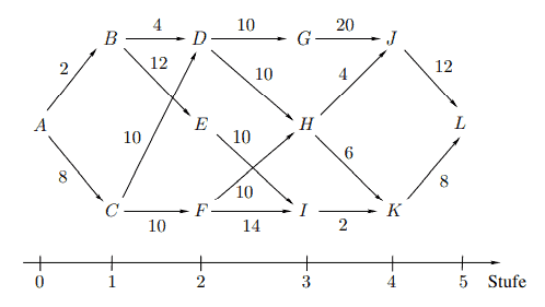
Wir ordnen den Orten $A, B, \ldots, L$ die Zustände $1,2, \ldots, 12$ zu und wählen als Aktionen die Zustände der direkten Nachfolgeorte. Da unserem Basismodell ein Maximierungsproblem zugrunde liegt, fassen wir die einstufigen Gewinne als die negativen Entfernungen der benachbarten Orte auf. Ausgehend vom terminalen Gewinn $V_5\left(s_5\right)=V_5(12)=0$ empfiehlt es sich, für jede Stufe eine Tabelle anzulegen, in diese Tabelle für jeden Zustand in Abhängigkeit von den zulässigen Aktionen die Werte der rechten Seite der Optimalitätsgleichung aufzunehmen und die sich aus der Auswertung ergebende Wertfunktion sowie die zugehörigen Maximalpunkte zu notieren. Der letzten Tabelle kann man dann $V_0\left(s_0\right)$ unmittelbar entnehmen und eine optimale Strategie durch Vorwärtsrechnung aus den bereitgestellten Daten leicht ermitteln.

数学代写|运筹学作业代写operational research代考|Anwendungsbereiche

Die bisherigen Beispiele zeigen bereits, dass die dynamische Optimierung eine sehr flexible Lösungstechnik ist, die sich auf die unterschiedlichsten Problemstellungen anwenden lässt. Voraussetzung für eine Anwendung ist lediglich, dass sich das Problem in Teilprobleme zerlegen lässt mit einer stufenweisen Abarbeitungsmöglichkeit. Eine solche Zerlegung ist bei dynamischen Entscheidungsproblemen in natürlicher Weise gegeben und kann darüber hinaus auch bei statischen Entscheidungsproblemen als alternativer Lösungsansatz (vgl. Bsp. 9.2) gezielt eingesetzt werden.
Den Vorteilen einer einfachen Darstellung, die sich in der Regel auf die Aufstellung der Optimalitätsgleichung beschränkt, und einer einfachen Rechenvorschrift steht der Nachteil eines erhöhten Rechen- und Speicheraufwandes gegenüber, der aus der Bereithaltung einer Vielzahl von Informationen bei der Behandlung und Verknüpfung der Teilprobleme entsteht.

Zu den klassischen Anwendungen deterministischer dynamischer Optimierungsprobleme gehören die Berechnung kürzester Wege in einem Netzwerk (vgl. Bsp. 9.1), die Berechnung längster Wege im Rahmen der Zeitplanung innerhalb der Netzplantechnik (vgl. Kap. 4), die optimale Aufteilung von Ressourcen (als Verallgemeinerung von Reispiel 9.2) sowie die Insgrößenplanung im Rahmen der Materialhereitstellungsplanung, auf die wir in dem folgenden Beispiel $9.5$ eingehen werden.

Die Bedarfsmengen $x_0, \ldots, x_{N-1}$ eines Gutes seien über einen Planungszeitraum von $N$ Perioden bekannt und jeweils am Ende der Periode bereitzustellen. Fehlmengen seien nicht zulässig. In Periode $n, n=0, \ldots, N-1$, können $a_n$ Einheiten des Gutes hergestellt werden. Diese stehen am Ende der Periode zur Verfügung. Verbunden mit der Herstellung sind Kosten der Höhe $c\left(a_n\right)$. Nicht unmittelbar benötigte Einheiten des Gutes können gelagert werden. Die Lagerkosten $l\left(s_n\right)$ in der Periode $n$ ergeben sich aus dem Lagerbestand $s_n$ zu Beginn der Periode. Zu Beginn der ersten Periode sei der Lagerbestand Null, ebenso am Ende der letzten Periode (d.h. $\left.s_0=s_N=0\right)$.

数学代写|运筹学作业代写operational research代考|MA3212

运筹学代考

数学代写|运筹学作业代写operational research代考|Wertiteration

根据定理 9.1,可以计算出最大总利润 $V_0\left(s_0\right)$ 以及最优策略的确定 $\delta^*$ 求解函数方程,最优方程。因此, 关于计算时间和内存要求的最优性方程的有效解是动态优化的中心任务之一。该定理可以是计算性的,例 如在算法中 $9.1$ 予以实施。
通过逆向计算,在算法中计算 $9.1$ 首先是价值函数 $V_{N-1}, \ldots, V_0$. 和 $V_{N-1}, \ldots, V_1$ 只需要一个迭代步 旧值函数 $v($ 步 $n+1)$ ,所以它有两个价值函数。
如果您想手动进行计算,在表格中进行计算是有意义的。为此,我们再举一个例子9.1在。特别是,我们 对确定性动态优化的基本模型进行了简化,并通过启发式考虑验证了已经实现的解决方案。
双柱式 9.4(Bcispicl9.1- 续 1).
我们安排地点 $A, B, \ldots, L$ 条件 $1,2, \ldots, 12$ 并选择直接后继位置的状态作为动作。由于我们的基本模型 基于最大化问题,我们将单级增益视为相邻位置的负距离。从终端利润开始 $V_5\left(s_5\right)=V_5(12)=0$ 建议 为每个阶段创建一个表,根据允许的操作,将每个状态的最优方程右侧的值包含在该表中,并注意评估产 生的价值函数和相关的最大点数。然后您可以使用最后一张表 $V_0\left(s_0\right)$ 通过根据提供的数据进行正向计 算,立即轻松地确定最佳策略。

数学代写|运筹学作业代写operational research代考|Anwendungsbereiche

前面的示例已经表明,动态优化是一种非常灵活的解决方案技术,可以应用于各种问题。对应用程序的唯 一要求是问题可以分解为具有逐步处理选项的子问题。这种分解在动态决策问题中以自然的方式给出,也 可以作为替代方法以有针对性的方式用于静态决策问题(参见示例 9.2)。
简单表示 (通常仅限于最优方程的建立) 和简单计算规则的优点被计算和存储成本增加的缺点所抵消,这 些缺点是在处理和处理时提供大量信息而引起的。连接子问题。
确定性动态优化问题的经典应用包括网络中最短路径的计算 (参见示例 9.1) 、网络规划技术中时间规划 框架内最长路径的计算 (参见第 4 章) 、最优资源分配(作为示例 $9.2$ 的概括) 以及在材料可用性规划框 架内规划总体规模,我们在以下示例中引用 $9.5$ 将进入。
所需数量 $x_0, \ldots, x_{N-1}$ 的商品超过了规划期 $N$ 已知的时期并将在每个时期结束时提供。不允许缺少数 量。在期间 $n, n=0, \ldots, N-1$ , 能够 $a_n$ 单位的商品被生产出来。这些在期末可用。与生产相关的是 高度的成本 $c\left(a_n\right)$. 可以存储不是立即需要的商品单元。存储成本 $l\left(s_n\right)$ 在期间 $n$ 清单的结果 $s_n$ 在期初。 在第一期开始时,库存为零,与上一期末的情况一样 (即 $\left.s_0=s_N=0\right)$.

统计代写|运筹学作业代写operational research代考 请认准statistics-lab™

统计代写请认准statistics-lab™. statistics-lab™为您的留学生涯保驾护航。

金融工程代写

金融工程是使用数学技术来解决金融问题。金融工程使用计算机科学、统计学、经济学和应用数学领域的工具和知识来解决当前的金融问题,以及设计新的和创新的金融产品。

非参数统计代写

非参数统计指的是一种统计方法,其中不假设数据来自于由少数参数决定的规定模型;这种模型的例子包括正态分布模型和线性回归模型。

广义线性模型代考

广义线性模型(GLM)归属统计学领域,是一种应用灵活的线性回归模型。该模型允许因变量的偏差分布有除了正态分布之外的其它分布。

术语 广义线性模型(GLM)通常是指给定连续和/或分类预测因素的连续响应变量的常规线性回归模型。它包括多元线性回归,以及方差分析和方差分析(仅含固定效应)。

有限元方法代写

有限元方法(FEM)是一种流行的方法,用于数值解决工程和数学建模中出现的微分方程。典型的问题领域包括结构分析、传热、流体流动、质量运输和电磁势等传统领域。

有限元是一种通用的数值方法,用于解决两个或三个空间变量的偏微分方程(即一些边界值问题)。为了解决一个问题,有限元将一个大系统细分为更小、更简单的部分,称为有限元。这是通过在空间维度上的特定空间离散化来实现的,它是通过构建对象的网格来实现的:用于求解的数值域,它有有限数量的点。边界值问题的有限元方法表述最终导致一个代数方程组。该方法在域上对未知函数进行逼近。[1] 然后将模拟这些有限元的简单方程组合成一个更大的方程系统,以模拟整个问题。然后,有限元通过变化微积分使相关的误差函数最小化来逼近一个解决方案。

tatistics-lab作为专业的留学生服务机构,多年来已为美国、英国、加拿大、澳洲等留学热门地的学生提供专业的学术服务,包括但不限于Essay代写,Assignment代写,Dissertation代写,Report代写,小组作业代写,Proposal代写,Paper代写,Presentation代写,计算机作业代写,论文修改和润色,网课代做,exam代考等等。写作范围涵盖高中,本科,研究生等海外留学全阶段,辐射金融,经济学,会计学,审计学,管理学等全球99%专业科目。写作团队既有专业英语母语作者,也有海外名校硕博留学生,每位写作老师都拥有过硬的语言能力,专业的学科背景和学术写作经验。我们承诺100%原创,100%专业,100%准时,100%满意。

随机分析代写


随机微积分是数学的一个分支,对随机过程进行操作。它允许为随机过程的积分定义一个关于随机过程的一致的积分理论。这个领域是由日本数学家伊藤清在第二次世界大战期间创建并开始的。

时间序列分析代写

随机过程,是依赖于参数的一组随机变量的全体,参数通常是时间。 随机变量是随机现象的数量表现,其时间序列是一组按照时间发生先后顺序进行排列的数据点序列。通常一组时间序列的时间间隔为一恒定值(如1秒,5分钟,12小时,7天,1年),因此时间序列可以作为离散时间数据进行分析处理。研究时间序列数据的意义在于现实中,往往需要研究某个事物其随时间发展变化的规律。这就需要通过研究该事物过去发展的历史记录,以得到其自身发展的规律。

回归分析代写

多元回归分析渐进(Multiple Regression Analysis Asymptotics)属于计量经济学领域,主要是一种数学上的统计分析方法,可以分析复杂情况下各影响因素的数学关系,在自然科学、社会和经济学等多个领域内应用广泛。

MATLAB代写

MATLAB 是一种用于技术计算的高性能语言。它将计算、可视化和编程集成在一个易于使用的环境中,其中问题和解决方案以熟悉的数学符号表示。典型用途包括:数学和计算算法开发建模、仿真和原型制作数据分析、探索和可视化科学和工程图形应用程序开发,包括图形用户界面构建MATLAB 是一个交互式系统,其基本数据元素是一个不需要维度的数组。这使您可以解决许多技术计算问题,尤其是那些具有矩阵和向量公式的问题,而只需用 C 或 Fortran 等标量非交互式语言编写程序所需的时间的一小部分。MATLAB 名称代表矩阵实验室。MATLAB 最初的编写目的是提供对由 LINPACK 和 EISPACK 项目开发的矩阵软件的轻松访问,这两个项目共同代表了矩阵计算软件的最新技术。MATLAB 经过多年的发展,得到了许多用户的投入。在大学环境中,它是数学、工程和科学入门和高级课程的标准教学工具。在工业领域,MATLAB 是高效研究、开发和分析的首选工具。MATLAB 具有一系列称为工具箱的特定于应用程序的解决方案。对于大多数 MATLAB 用户来说非常重要,工具箱允许您学习应用专业技术。工具箱是 MATLAB 函数(M 文件)的综合集合,可扩展 MATLAB 环境以解决特定类别的问题。可用工具箱的领域包括信号处理、控制系统、神经网络、模糊逻辑、小波、仿真等。

R语言代写问卷设计与分析代写
PYTHON代写回归分析与线性模型代写
MATLAB代写方差分析与试验设计代写
STATA代写机器学习/统计学习代写
SPSS代写计量经济学代写
EVIEWS代写时间序列分析代写
EXCEL代写深度学习代写
SQL代写各种数据建模与可视化代写

数学代写|运筹学作业代写operational research代考|MAT2200

statistics-lab™ 为您的留学生涯保驾护航 在代写运筹学operational research方面已经树立了自己的口碑, 保证靠谱, 高质且原创的统计Statistics代写服务。我们的专家在代写运筹学operational research代写方面经验极为丰富,各种代写运筹学operational research相关的作业也就用不着说。

我们提供的运筹学operational research及其相关学科的代写,服务范围广, 其中包括但不限于:

  • Statistical Inference 统计推断
  • Statistical Computing 统计计算
  • Advanced Probability Theory 高等楖率论
  • Advanced Mathematical Statistics 高等数理统计学
  • (Generalized) Linear Models 广义线性模型
  • Statistical Machine Learning 统计机器学习
  • Longitudinal Data Analysis 纵向数据分析
  • Foundations of Data Science 数据科学基础
数学代写|运筹学作业代写operational research代考|MAT2200

数学代写|运筹学作业代写operational research代考|Das Optimalitätskriterium

Bei Anwendung einer Strategie $\delta=\left(a_0, a_1, \ldots, a_{N-1}\right)$ ergibt sich der Gesamtgewinn
$$
R_\delta\left(s_0\right):=\sum_{n=0}^{N-1} r_n\left(s_n, a_n\right)+V_N\left(s_N\right) .
$$
Eine Strategie $\delta^$ heißt optimal, falls $R_{\delta^}\left(s_0\right) \geq R_\delta\left(s_0\right)$ für alle $\delta \in \Delta$ gilt. Man überprüft leicht, dass die Menge $\Delta$ endlich ist, da der Anfangszustand $s_0$ fest ist und neben dem Planungshorizont auch die Mengen zulässiger Aktionen endlich sind. Somit existiert stets eine optimale Strategie.
Die Berechnung des maximalen Gesamtgewinns
$$
V_0\left(s_0\right):=\max \left{R_\delta\left(s_0\right) \mid \delta \in \Delta\right}
$$
und die Ermittlung einer optimalen Strategie $\delta^*$ lassen sich auf die Lösung einer Funktionalgleichung, der sogenannten Optimalitätsgleichung, auch Bellmansche Funktionalgleichung genannt, zurückführen.

Zur Herleitung benötigen wir noch den maximalen Gewinn ab Stufe $n$ in Abhängigkeit vom Zustand $s_n \in \mathcal{S}n$, also $$ \begin{gathered} V_n\left(s_n\right):=\max \left{\sum{t=n}^{N-1} r_t\left(s_t, a_t\right)+V_N\left(s_N\right) \mid a_n \in \mathcal{A}n\left(s_n\right),\right. \ \left.\ldots, a{N-1} \in \mathcal{A}{N-1}\left(s{N-1}\right)\right}
\end{gathered}
$$
Dabei ist $s_{n+1}=z_n\left(s_n, a_n\right), \ldots, s_N=z_{N-1}\left(s_{N-1}, a_{N-1}\right)$. Die Funktionen $V_0, \ldots, V_N$ bezeichnet man auch als Wertfunktionen.

数学代写|运筹学作业代写operational research代考|Die Optimalitätsgleichung

Wir erhalten nun das zentrale Ergebnis dieses Abschnitts.
Satz 9.1. (Optimalitütsgleichung)
(i) Für $n=0, \ldots, N-1$ und alle $s_n \in \mathcal{S}n$ gilt $$ V_n\left(s_n\right)=\max {a \in \mathcal{A}n\left(s_n\right)}\left{r_n\left(s_n, a\right)+V{n+1}\left(z_n\left(s_n, a\right)\right)\right} .
$$
(ii) Definiert man aus den die rechte Seite von (9.1) maximierenden Aktionen rekursiv eine Aktionenfolge $a_0^, a_1^, \ldots, a_{N-1}^$ gemä $\beta$ $$ r_0\left(s_0, a_0^\right)+V_1\left(z_0\left(s_0, a_0^\right)\right)=\max \left{r_0\left(s_0, a\right)+V_1\left(z_0\left(s_0, a\right)\right) \mid a \in \mathcal{A}0\left(s_0\right)\right} $$ und für $n-1,2, \ldots, N-1, s_n-z{n-1}\left(s_{n-1}, a_{n-1}^\right)$ gemä $\beta$
$$
\begin{aligned}
& r_n\left(s_n, a_n^\right)+V_{n+1}\left(z_n\left(s_n, a_n^\right)\right)= \
& \max \left{r_n\left(s_n, a\right)+V_{n+1}\left(z_n\left(s_n, a\right)\right) \mid a \in \mathcal{A}n\left(s_n\right)\right}, \end{aligned} $$ so ist die zugehörige Strategie $\delta^=\left(a_0^, \ldots, a{N-1}^*\right)$ optimal.

Beweis. (i) Sei $n \in{0, \ldots, N-1}, s_n \in \mathcal{S}n$. Da $\Delta$ endlich ist, existiert eine ab Stufe $n$ optimale Aktionenfolge $\left(a_n^, \ldots, a{N-1}^\right)$ und eine zugehörige Zustandsfolge $s_n^=s_n, s_{n+1}^=z_n\left(s_n^, a_n^\right), \ldots, s_N^=z_{N-1}\left(s_{N-1}^, a_{N-1}^\right)$ mit $$ \begin{aligned} V_n\left(s_n\right) & =\sum_{t=n}^{N-1} r_t\left(s_t^, a_t^\right)+V_N\left(s_N^\right) \
& =r_n\left(s_n, a_n^\right)+\sum_{t=n+1}^{N-1} r_t\left(s_t^, a_t^\right)+V_N\left(s_N^\right),
\end{aligned}
$$
und wir erhalten die Abschätzung
$$
\begin{aligned}
V_n\left(s_n\right) & \leq r_n\left(s_n, a_n^\right)+V_{n+1}\left(z_n\left(s_n, a_n^\right)\right) \
& \leq \max \left{r_n\left(s_n, a\right)+V_{n+1}\left(z_n\left(s_n, a\right)\right) \mid a \in \mathcal{A}_n\left(s_n\right)\right}
\end{aligned}
$$

数学代写|运筹学作业代写operational research代考|MAT2200

运筹学代考

数学代写|运筹学作业代写operational research代考|Das Optimalitätskriterium

应用策略时 $\delta=\left(a_0, a_1, \ldots, a_{N-1}\right)$ 给出总利润
$$
R_\delta\left(s_0\right):=\sum_{n=0}^{N-1} r_n\left(s_n, a_n\right)+V_N\left(s_N\right) .
$$
适用。一个人很容易检查那个数额 $\Delta$ 有限是因为初始状态 $s_0$ 是固定的,除了规划范围之外,允许的行动 数量也是有限的。因此,总是存在最优策略。
最大利润总额的计算
V_olleft(s_OIright):=Imax \left(R__Ideltalleft(s_OIright) \mid \delta lin \Deltalright}
以及最优策略的确定 $\delta^*$ 可以追溯到一个函数方程的解,即所谓的最优方程,也称为贝尔曼函数方程。
对于推导,我们仍然需要水平的最大增益 $n$ 视情况而定 $s_n \in \mathcal{S} n$ ,还
有 $s_{n+1}=z_n\left(s_n, a_n\right), \ldots, s_N=z_{N-1}\left(s_{N-1}, a_{N-1}\right)$. 功能 $V_0, \ldots, V_N$ 也称为价值函数。

数学代写|运筹学作业代写operational research代考|Die Optimalitätsgleichung

我们现在得到了本节的主要结果。
定理 9.1。(最优方程)
(i) Forn $=0, \ldots, N-1$ 和所有 $s_n \in \mathcal{S} n$ 适用
(ii) 从最大化 $(9.1)$ 右侧的动作递归定义一系列动作。 $a_{-} 0^{\wedge}, a_{-} 1^{\wedge} , \backslash d o t s, a_{-}{N-1}^{\wedge}$ 根据 $\beta$
\begin{aligned } } \text { \& r_n\left(s_n, a_ } n ^ { \wedge } \backslash r i g h t ) + V _ { – } { n + 1 } \backslash l e f t ( z _ { – } n \backslash l e f t ( s _ { – } n , a _ { – } n ^ { \wedge } \backslash r i g h t ) \backslash r i g h t ) = \backslash \& \backslash m a x \backslash l
这是相关的策略 $\delta^{=}\left(a_0^{\prime} \ldots, a N-1^*\right)$ 最佳的。
证明。(i) 成为 $n \in 0, \ldots, N-1, s_n \in \mathcal{S} n$. 和 $\Delta$ 是有限的,有一个ab层 $n$ 最佳行动顺序
\eft(a_ $n^{\wedge}$, Vdots, $a{N-1}^{\wedge} \backslash$ right $)$ 和一个相关的状态序列
我们得到了估计

统计代写|运筹学作业代写operational research代考 请认准statistics-lab™

统计代写请认准statistics-lab™. statistics-lab™为您的留学生涯保驾护航。

金融工程代写

金融工程是使用数学技术来解决金融问题。金融工程使用计算机科学、统计学、经济学和应用数学领域的工具和知识来解决当前的金融问题,以及设计新的和创新的金融产品。

非参数统计代写

非参数统计指的是一种统计方法,其中不假设数据来自于由少数参数决定的规定模型;这种模型的例子包括正态分布模型和线性回归模型。

广义线性模型代考

广义线性模型(GLM)归属统计学领域,是一种应用灵活的线性回归模型。该模型允许因变量的偏差分布有除了正态分布之外的其它分布。

术语 广义线性模型(GLM)通常是指给定连续和/或分类预测因素的连续响应变量的常规线性回归模型。它包括多元线性回归,以及方差分析和方差分析(仅含固定效应)。

有限元方法代写

有限元方法(FEM)是一种流行的方法,用于数值解决工程和数学建模中出现的微分方程。典型的问题领域包括结构分析、传热、流体流动、质量运输和电磁势等传统领域。

有限元是一种通用的数值方法,用于解决两个或三个空间变量的偏微分方程(即一些边界值问题)。为了解决一个问题,有限元将一个大系统细分为更小、更简单的部分,称为有限元。这是通过在空间维度上的特定空间离散化来实现的,它是通过构建对象的网格来实现的:用于求解的数值域,它有有限数量的点。边界值问题的有限元方法表述最终导致一个代数方程组。该方法在域上对未知函数进行逼近。[1] 然后将模拟这些有限元的简单方程组合成一个更大的方程系统,以模拟整个问题。然后,有限元通过变化微积分使相关的误差函数最小化来逼近一个解决方案。

tatistics-lab作为专业的留学生服务机构,多年来已为美国、英国、加拿大、澳洲等留学热门地的学生提供专业的学术服务,包括但不限于Essay代写,Assignment代写,Dissertation代写,Report代写,小组作业代写,Proposal代写,Paper代写,Presentation代写,计算机作业代写,论文修改和润色,网课代做,exam代考等等。写作范围涵盖高中,本科,研究生等海外留学全阶段,辐射金融,经济学,会计学,审计学,管理学等全球99%专业科目。写作团队既有专业英语母语作者,也有海外名校硕博留学生,每位写作老师都拥有过硬的语言能力,专业的学科背景和学术写作经验。我们承诺100%原创,100%专业,100%准时,100%满意。

随机分析代写


随机微积分是数学的一个分支,对随机过程进行操作。它允许为随机过程的积分定义一个关于随机过程的一致的积分理论。这个领域是由日本数学家伊藤清在第二次世界大战期间创建并开始的。

时间序列分析代写

随机过程,是依赖于参数的一组随机变量的全体,参数通常是时间。 随机变量是随机现象的数量表现,其时间序列是一组按照时间发生先后顺序进行排列的数据点序列。通常一组时间序列的时间间隔为一恒定值(如1秒,5分钟,12小时,7天,1年),因此时间序列可以作为离散时间数据进行分析处理。研究时间序列数据的意义在于现实中,往往需要研究某个事物其随时间发展变化的规律。这就需要通过研究该事物过去发展的历史记录,以得到其自身发展的规律。

回归分析代写

多元回归分析渐进(Multiple Regression Analysis Asymptotics)属于计量经济学领域,主要是一种数学上的统计分析方法,可以分析复杂情况下各影响因素的数学关系,在自然科学、社会和经济学等多个领域内应用广泛。

MATLAB代写

MATLAB 是一种用于技术计算的高性能语言。它将计算、可视化和编程集成在一个易于使用的环境中,其中问题和解决方案以熟悉的数学符号表示。典型用途包括:数学和计算算法开发建模、仿真和原型制作数据分析、探索和可视化科学和工程图形应用程序开发,包括图形用户界面构建MATLAB 是一个交互式系统,其基本数据元素是一个不需要维度的数组。这使您可以解决许多技术计算问题,尤其是那些具有矩阵和向量公式的问题,而只需用 C 或 Fortran 等标量非交互式语言编写程序所需的时间的一小部分。MATLAB 名称代表矩阵实验室。MATLAB 最初的编写目的是提供对由 LINPACK 和 EISPACK 项目开发的矩阵软件的轻松访问,这两个项目共同代表了矩阵计算软件的最新技术。MATLAB 经过多年的发展,得到了许多用户的投入。在大学环境中,它是数学、工程和科学入门和高级课程的标准教学工具。在工业领域,MATLAB 是高效研究、开发和分析的首选工具。MATLAB 具有一系列称为工具箱的特定于应用程序的解决方案。对于大多数 MATLAB 用户来说非常重要,工具箱允许您学习应用专业技术。工具箱是 MATLAB 函数(M 文件)的综合集合,可扩展 MATLAB 环境以解决特定类别的问题。可用工具箱的领域包括信号处理、控制系统、神经网络、模糊逻辑、小波、仿真等。

R语言代写问卷设计与分析代写
PYTHON代写回归分析与线性模型代写
MATLAB代写方差分析与试验设计代写
STATA代写机器学习/统计学习代写
SPSS代写计量经济学代写
EVIEWS代写时间序列分析代写
EXCEL代写深度学习代写
SQL代写各种数据建模与可视化代写

数学代写|运筹学作业代写operational research代考|MATH3202

statistics-lab™ 为您的留学生涯保驾护航 在代写运筹学operational research方面已经树立了自己的口碑, 保证靠谱, 高质且原创的统计Statistics代写服务。我们的专家在代写运筹学operational research代写方面经验极为丰富,各种代写运筹学operational research相关的作业也就用不着说。

我们提供的运筹学operational research及其相关学科的代写,服务范围广, 其中包括但不限于:

  • Statistical Inference 统计推断
  • Statistical Computing 统计计算
  • Advanced Probability Theory 高等楖率论
  • Advanced Mathematical Statistics 高等数理统计学
  • (Generalized) Linear Models 广义线性模型
  • Statistical Machine Learning 统计机器学习
  • Longitudinal Data Analysis 纵向数据分析
  • Foundations of Data Science 数据科学基础
数学代写|运筹学作业代写operational research代考|MATH3202

数学代写|运筹学作业代写operational research代考|Dynamische Optimierung

Mehrstufige Entscheidungsprobleme begegnen uns im Alltag ständig. Sie treten immer dann auf, wenn eine zu treffende Entscheidung neben unmittelbaren Auswirkungen auch Konsequenzen auf zukünftige Entscheidungen haben kann. Wir haben es also nicht mit isoliert zu betrachtenden Entscheidungen zu tun, sondern mit einer Folge von Entscheidungen, die in einem engen Zusammenhang stehen. Das folgende einfache Beispiel verdeutlicht die Problematik: Ein Langstreckenläufer, der sich zum Ziel gesetzt hat, eine Meisterschaft zu erringen, wird dieses Ziel verfehlen, wenn er sich taktisch falsch verhält. Geht er das Rennen zu schnell an, so wird er das Tempo nicht durchhalten können und in der Endphase des Rennens zurückfallen. Geht er umgekehrt das Rennen zu langsam an und wird der Abstand zur Spitzengruppe zu groß, so wird er den Rückstand nicht mehr aufholen können. Er wird sich daher die Strecke gedanklich in Abschnitte einteilen und in jedem Abschnitt sein Laufverhalten auf das der Konkurrenten um den Titel und seine Leistungsfähigkeit abstimmen.

Die dynamische Optimierung ist ein rekursives Verfahren zur Lösung mehrstufiger Entscheidungsprobleme. Streng genommen ist sie eine Lösungstechnik, die auf ein konkretes Problem, das sich in Teilprobleme zerlegen lässt, angepasst wird. Verknüpft sind diese Teilprobleme über eine Struktur, die es erlaubt, die Teilprobleme rekursiv zu lösen und die gefundenen Teillösungen zu einer Gesamtlösung zusammenzusetzen. Die folgenden Beispiele dienen der Verdeutlichung. Die Vorgehensweise orientiert sich allein an der Anschauung. Eine formale Überprüfung und Rechtfertigung wird in den nachfolgenden Abschnitten vorgenommen.

Der Weg von $A$ nach $L$ lässt sich, unabhängig von den tatsächlich angefahrenen Orten, in fünf Teilstrecken (direkte Verbindungen) zerlegen. Die zugehörigen Orte als Anfangs- oder Zielorte der Teilstrecken lauten $A$ (Stufe 0), $B$ und $C$ (Stufe 1), $D, E$ und $F$ (Stufe 2), $G, H$ und $I$ (Stufe 3), $J$ und $K$ (Stufe 4) und schließlich $L$ (Stufe 5).

Den Bewertungen der Pfeile entnehmen wir die Entfernungen der Teilstrecken. Um die kürzeste Verbindung zwischen den Orten $A$ und $L$ zu bestimmen, unterstellen wir zunächst, dass wir bereits einen Ort der Stufe $n$ erreicht haben und, ausgehend von diesem Ort $s$, den kürzesten Restweg nach $L$ suchen, dessen Länge wir mit $V_n(s)$ bezeichnen wollen. Für $n=0$ und somit für den Anfangsort $s=A$ geht dann der kürzeste Restweg $V_0(A)$ in die gesuchte kürzeste Verbindung zwischen den Orten $A$ und $L$ über.

Die direkte Verbindung zwischen den Orten $J$ und $K$ der Stufe 4 und dem Zielort $L$ ergibt unmittelbar $V_4(J)=12$ bzw. $V_4(K)=8$

数学代写|运筹学作业代写operational research代考|Deterministische dynamische Optimierung

Unter einem endlich-stufigen deterministischen dynamischen Optimierungsproblem verstehen wir ein Tupel $\left(N, \mathcal{S}, \mathcal{A}, z, r, V_N\right)$, wobei die einzelnen GröBen die folgende Bedeutung haben:
(i) $N \in \mathbb{N}$, der Planungshorizont, legt die Anzahl der Stufen fest $(n=$ $0,1, \ldots, N)$.
(ii) $\mathcal{S}$, der Zustandsraum, ist eine abzählbare Menge. Die nichtleeren Teilmengen $\mathcal{S}0=\left{s_0\right}, \mathcal{S}_1, \ldots, \mathcal{S}_N$ sind die Zustandsmengen der Stufen $0,1, \ldots, N$. (iii) $\mathcal{A}$, der Aktionenraum, ist eine abzählbare Menge. Die nichtleeren endlichen Teilmengen $\mathcal{A}_n(s), s \in \mathcal{S}_n$, sind die vom Zustand $s$ und der Stufe $n{n+1}$, die Zustandstransformation, ist eine Funktion, die jedem Zustand $s \in \mathcal{S}n$ und jeder zulässigen Aktion $a \in \mathcal{A}_n(s)$ den neuen Zustand $s^{\prime}=z_n(s, a) \in \mathcal{S}{n+1}$ zuordnet $(n<N)$.
(v) $r_n: \mathcal{D}n \rightarrow \mathbb{R}$, die einstufige Gewinnfunktion, ist eine Funktion, die den einstufigen Gewinn $r{n u}(s, a)$ im Zustand $s \in \mathcal{S}_n$ bei Wahl der Aktion $a \in \mathcal{A}_u(s)$ angibt $(n<N)$.
(vi) $V_N: S_N \rightarrow \mathbb{R}$, die terminale Gewinnfunktion, ist eine Funktion, die auf Stufe $N$ den terminalen Gewinn $V_N(s)$ im Zustand $s \in \mathcal{S}_N$ angibt.

Abbildung $9.2$ illustriert, wie Zustände eines endlich-stufigen deterministischen dynamischen Optimierungsproblems miteinander verknüpft sein können.

Die Stufen $n=0,1, \ldots, N$ eines dynamischen Optimierungsproblems kann man häufig als diskrete Zeitpunkte interpretieren, zu denen ein System beobachtet wird. Befindet sich ein solches System zum Zeitpunkt $n<N$ im Zustand $s$, so wählt der Beobachter eine zulässige Aktion $a \in \mathcal{A}_n(s)$. Verbunden mit dem Zustand $s$ und der Wahl der Aktion $a$ ist ein einstufiger Gewinn $r_n(s, a)$, und das System geht über in den Zustand $s^{\prime}=z_n(s, a)$ zum Zeitpunkt $n+1$ (vgl. Abb. 9.3).

数学代写|运筹学作业代写operational research代考|MATH3202

运筹学代考

数学代写|运筹学作业代写operational research代考|Dynamische Optimierung

我们在日常生活中不断遇到多阶段决策问题。当要做出的决定除了直接影响外,还会对末来的决定产生影 响时,它们总是会发生。因此,我们不是在处理要孤立考虑的决策,而是在处理一系列密切相关的决策。 下面这个简单的例子就说明了这个问题: 一个给自己定下夺冠目标的长跑运动员,如果他在战术上的表现 不对,就会与这个目标失之交臂。如果他起步太快,他将跟不上步伐,会在比寒的最后阶段落后。相反, 如果他起步太慢,与领先集团的差距变得太大,所以他将无法赶上。因此,他会在心理上将路线分成几个 部分,并调整自己的跑步行为以适应他的竞争对手的标题和他在每个部分的表现。
动态优化是解决多层次决策问题的一种递归方法。严格地说,它是一种适用于可以分解为子问题的特定问 题的解决技术。这些部分问题通过一种结构联系起来,该结构允许递归地解决部分问题,并将找到的部分 解决方案组合成一个整体解决方案。提供以下示例以进行说明。该过程完全基于直觉。以下部分提供了正 式的审查和理由。
的方式从 $A$ 后 $L$ 可以分为五个部分(直接连接),而不管实际旅行到的位置。相关位置作为部分的开始或 目标位置如下 $A$ (0级), $B$ 和 $C$ (步骤 1 ) , $D, E$ 和 $F$ (2级) , $G, H$ 和 $I$ (3级), $J$ 和 $K$ (第 4 阶 段)最后 $L$ (5 级)。
我们从箭头的等级中获取部分的距离。提供地点之间的最短路线 $A$ 和 $L$ 为了确定,我们首先假设我们已经 有了舞台的位置 $n$ 已经到达,从这里开始 $s$, 最短距离 $L$ 寻找我们正在使用的长度 $V_n(s)$ 想指定。为了 $n=0$ 因此作为起点 $s=A$ 那么最短的距离 $V_0(A)$ 进入位置之间的最短连接 $A$ 和 $L$ 超过。
地方之间的直接联系 $J$ 和 $K$ 4级和目的地 $L$ 马上出结果 $V_4(J)=12$ 分别。 $V_4(K)=8$

数学代写|运筹学作业代写operational research代考|Deterministische dynamische Optimierung

我们所说的有限级确定性动态优化问题是指一个元组 $\left(N, \mathcal{S}, \mathcal{A}, z, r, V_N\right)$ ,其中各个数量具有以下含 义:
(i) $N \in \mathbb{N}$ ,规划范围,决定层数 $(n=0,1, \ldots, N)$.
(二) $\mathcal{S}$ ,状态空间,是一个可数集。非空子集
作空间,是一个可数集。非空有限子集 $\mathcal{A}_n(s), s \in \mathcal{S}_n$ ,是国家的 $s$ 和水平 $n n+1$ ,状态转换,是与每个 状态相关联的函数 $s \in \mathcal{S} n$ 以及任何允许的行为 $a \in \mathcal{A}_n(s)$ 新状态 $s^{\prime}=z_n(s, a) \in \mathcal{S} n+1$ 指派 $(n<N)$.
(在) $r_n: \mathcal{D} n \rightarrow \mathbb{R}$, the one-level profit function, 是计算一级利润的函数 $r n u(s, a)$ 在条件 $s \in \mathcal{S}_n$ 选择动作时 $a \in \mathcal{A}_u(s)$ 表明 $(n<N)$.
(我们) $V_N: S_N \rightarrow \mathbb{R}$ ,终端利润函数,是一个基于水平的函数 $N$ 终端利润 $V_N(s)$ 在条件 $s \in \mathcal{S}_N$ 表 明。
揷图9.2说明了如何链接有限级确定性动态优化问题的状态。
步骤 $n=0,1, \ldots, N$ 动态优化问题的时间点通常可以解释为观察系统的离散时间点。当时有没有这样 的系统 $n<N$ 在条件 $s$ ,观察者选择一个法律行动 $a \in \mathcal{A}_n(s)$. 与国家有关 $s$ 和行动的选择 $a$ 是一步胜利 $r_n(s, a)$ ,系统转移到状态 $s^{\prime}=z_n(s, a)$ 当时 $n+1$ (见图 9.3)。

统计代写|运筹学作业代写operational research代考 请认准statistics-lab™

统计代写请认准statistics-lab™. statistics-lab™为您的留学生涯保驾护航。

金融工程代写

金融工程是使用数学技术来解决金融问题。金融工程使用计算机科学、统计学、经济学和应用数学领域的工具和知识来解决当前的金融问题,以及设计新的和创新的金融产品。

非参数统计代写

非参数统计指的是一种统计方法,其中不假设数据来自于由少数参数决定的规定模型;这种模型的例子包括正态分布模型和线性回归模型。

广义线性模型代考

广义线性模型(GLM)归属统计学领域,是一种应用灵活的线性回归模型。该模型允许因变量的偏差分布有除了正态分布之外的其它分布。

术语 广义线性模型(GLM)通常是指给定连续和/或分类预测因素的连续响应变量的常规线性回归模型。它包括多元线性回归,以及方差分析和方差分析(仅含固定效应)。

有限元方法代写

有限元方法(FEM)是一种流行的方法,用于数值解决工程和数学建模中出现的微分方程。典型的问题领域包括结构分析、传热、流体流动、质量运输和电磁势等传统领域。

有限元是一种通用的数值方法,用于解决两个或三个空间变量的偏微分方程(即一些边界值问题)。为了解决一个问题,有限元将一个大系统细分为更小、更简单的部分,称为有限元。这是通过在空间维度上的特定空间离散化来实现的,它是通过构建对象的网格来实现的:用于求解的数值域,它有有限数量的点。边界值问题的有限元方法表述最终导致一个代数方程组。该方法在域上对未知函数进行逼近。[1] 然后将模拟这些有限元的简单方程组合成一个更大的方程系统,以模拟整个问题。然后,有限元通过变化微积分使相关的误差函数最小化来逼近一个解决方案。

tatistics-lab作为专业的留学生服务机构,多年来已为美国、英国、加拿大、澳洲等留学热门地的学生提供专业的学术服务,包括但不限于Essay代写,Assignment代写,Dissertation代写,Report代写,小组作业代写,Proposal代写,Paper代写,Presentation代写,计算机作业代写,论文修改和润色,网课代做,exam代考等等。写作范围涵盖高中,本科,研究生等海外留学全阶段,辐射金融,经济学,会计学,审计学,管理学等全球99%专业科目。写作团队既有专业英语母语作者,也有海外名校硕博留学生,每位写作老师都拥有过硬的语言能力,专业的学科背景和学术写作经验。我们承诺100%原创,100%专业,100%准时,100%满意。

随机分析代写


随机微积分是数学的一个分支,对随机过程进行操作。它允许为随机过程的积分定义一个关于随机过程的一致的积分理论。这个领域是由日本数学家伊藤清在第二次世界大战期间创建并开始的。

时间序列分析代写

随机过程,是依赖于参数的一组随机变量的全体,参数通常是时间。 随机变量是随机现象的数量表现,其时间序列是一组按照时间发生先后顺序进行排列的数据点序列。通常一组时间序列的时间间隔为一恒定值(如1秒,5分钟,12小时,7天,1年),因此时间序列可以作为离散时间数据进行分析处理。研究时间序列数据的意义在于现实中,往往需要研究某个事物其随时间发展变化的规律。这就需要通过研究该事物过去发展的历史记录,以得到其自身发展的规律。

回归分析代写

多元回归分析渐进(Multiple Regression Analysis Asymptotics)属于计量经济学领域,主要是一种数学上的统计分析方法,可以分析复杂情况下各影响因素的数学关系,在自然科学、社会和经济学等多个领域内应用广泛。

MATLAB代写

MATLAB 是一种用于技术计算的高性能语言。它将计算、可视化和编程集成在一个易于使用的环境中,其中问题和解决方案以熟悉的数学符号表示。典型用途包括:数学和计算算法开发建模、仿真和原型制作数据分析、探索和可视化科学和工程图形应用程序开发,包括图形用户界面构建MATLAB 是一个交互式系统,其基本数据元素是一个不需要维度的数组。这使您可以解决许多技术计算问题,尤其是那些具有矩阵和向量公式的问题,而只需用 C 或 Fortran 等标量非交互式语言编写程序所需的时间的一小部分。MATLAB 名称代表矩阵实验室。MATLAB 最初的编写目的是提供对由 LINPACK 和 EISPACK 项目开发的矩阵软件的轻松访问,这两个项目共同代表了矩阵计算软件的最新技术。MATLAB 经过多年的发展,得到了许多用户的投入。在大学环境中,它是数学、工程和科学入门和高级课程的标准教学工具。在工业领域,MATLAB 是高效研究、开发和分析的首选工具。MATLAB 具有一系列称为工具箱的特定于应用程序的解决方案。对于大多数 MATLAB 用户来说非常重要,工具箱允许您学习应用专业技术。工具箱是 MATLAB 函数(M 文件)的综合集合,可扩展 MATLAB 环境以解决特定类别的问题。可用工具箱的领域包括信号处理、控制系统、神经网络、模糊逻辑、小波、仿真等。

R语言代写问卷设计与分析代写
PYTHON代写回归分析与线性模型代写
MATLAB代写方差分析与试验设计代写
STATA代写机器学习/统计学习代写
SPSS代写计量经济学代写
EVIEWS代写时间序列分析代写
EXCEL代写深度学习代写
SQL代写各种数据建模与可视化代写

计算机代写|机器学习代写machine learning代考|COMP4702

如果你也在 怎样代写机器学习 machine learning这个学科遇到相关的难题,请随时右上角联系我们的24/7代写客服。

机器学习是一个致力于理解和建立 “学习 “方法的研究领域,也就是说,利用数据来提高某些任务的性能的方法。机器学习算法基于样本数据(称为训练数据)建立模型,以便在没有明确编程的情况下做出预测或决定。机器学习算法被广泛用于各种应用,如医学、电子邮件过滤、语音识别和计算机视觉,在这些应用中,开发传统算法来执行所需任务是困难的或不可行的。

statistics-lab™ 为您的留学生涯保驾护航 在代写机器学习 machine learning方面已经树立了自己的口碑, 保证靠谱, 高质且原创的统计Statistics代写服务。我们的专家在代写机器学习 machine learning代写方面经验极为丰富,各种代写机器学习 machine learning相关的作业也就用不着说。

我们提供的机器学习 machine learning及其相关学科的代写,服务范围广, 其中包括但不限于:

  • Statistical Inference 统计推断
  • Statistical Computing 统计计算
  • Advanced Probability Theory 高等概率论
  • Advanced Mathematical Statistics 高等数理统计学
  • (Generalized) Linear Models 广义线性模型
  • Statistical Machine Learning 统计机器学习
  • Longitudinal Data Analysis 纵向数据分析
  • Foundations of Data Science 数据科学基础
计算机代写|机器学习代写machine learning代考|COMP4702

计算机代写|机器学习代写machine learning代考|Intuition and Main Results

Consider first the training error $E_{\text {train }}$ defined in (5.3). Since
$$
\operatorname{tr} \mathbf{Y} \mathbf{Q}^2(\gamma) \mathbf{Y}^{\boldsymbol{\top}}=-\frac{\partial}{\partial \gamma} \operatorname{tr} \mathbf{Y} \mathbf{Q}(\gamma) \mathbf{Y}^{\top},
$$
a deterministic equivalent for the resolvent $\mathbf{Q}(\gamma)$ is sufficient to acceess the asymptotic behavior of $E_{\text {train }}$.
With a linear activation $\sigma(t)=t$, the resolvent of interest
$$
\mathbf{Q}(\gamma)=\left(\frac{1}{n} \sigma(\mathbf{W X})^{\top} \sigma(\mathbf{W} \mathbf{X})+\gamma \mathbf{I}n\right)^{-1} $$ is the same as in Theorem 2.6. In a sense, the evaluation of $\mathbf{Q}(\gamma)$ (and subsequently $\left.E{\text {train }}\right)$ calls for an extension of Theorem $2.6$ to handle the case of nonlinear activations. Recall now that the main ingredients to derive a deterministic equivalent for (the linear case) $\mathbf{Q}=\left(\mathbf{X}^{\top} \mathbf{W}^{\top} \mathbf{W} \mathbf{X} / n+\gamma \mathbf{I}n\right)^{-1}$ are (i) $\mathbf{X}^{\top} \mathbf{W}^{\top}$ has i.i.d. columns and (ii) its $i$ th column $\left[\mathbf{W}^{\top}\right]_i$ has i.i.d. (or linearly dependent) entries so that the key Lemma $2.11$ applies. These hold, in the linear case, due to the i.i.d. property of the entries of $\mathbf{W}$. However, while for Item (i), the nonlinear $\Sigma^{\top}=\sigma(\mathbf{W X})^{\top}$ still has i.i.d. columns, and for Item (ii), its $i$ th column $\sigma\left(\left[\mathbf{X}^{\top} \mathbf{W}^{\top}\right]{. i}\right)$ no longer has i.i.d. or linearly dependent entries. Therefore, the main technical difficulty here is to obtain a nonlinear version of the trace lemma, Lemma 2.11. That is, we expect that the concentration of quadratic forms around their expectation remains valid despite the application of the entry-wise nonlinear $\sigma$. This naturally falls into the concentration of measure theory discussed in Section $2.7$ and is given by the following lemma.

Lemma 5.1 (Concentration of nonlinear quadratic form, Louart et al. [2018, Lemma 1]). For $\mathbf{w} \sim \mathcal{N}\left(\mathbf{0}, \mathbf{I}_p\right)$, 1-Lipschitz $\sigma(\cdot)$, and $\mathbf{A} \in \mathbb{R}^{n \times n}, \mathbf{X} \in \mathbb{R}^{p \times n}$ such that $|\mathbf{A}| \leq 1$ and $|\mathbf{X}|$ bounded with respect to $p, n$, then,
$$
\mathbb{P}\left(\left|\frac{1}{n} \sigma\left(\mathbf{w}^{\top} \mathbf{X}\right) \mathbf{A} \sigma\left(\mathbf{X}^{\top} \mathbf{w}\right)-\frac{1}{n} \operatorname{tr} \mathbf{A} \mathbf{K}\right|>t\right) \leq C e^{-c n \min \left(t, t^2\right)}
$$ for some $C, c>0, p / n \in(0, \infty)$ with ${ }^2$
$$
\mathbf{K} \equiv \mathbf{K}{\mathbf{X X}} \equiv \mathbb{E}{\mathbf{w} \sim \mathcal{N}\left(\mathbf{0}, \mathbf{I}_p\right)}\left[\sigma\left(\mathbf{X}^{\top} \mathbf{w}\right) \sigma\left(\mathbf{w}^{\boldsymbol{\top}} \mathbf{X}\right)\right] \in \mathbb{R}^{n \times n}
$$

计算机代写|机器学习代写machine learning代考|Consequences for Learning with Large Neural Networks

To validate the asymptotic analysis in Theorem $5.1$ and Corollary $5.1$ on real-world data, Figures $5.2$ and $5.3$ compare the empirical MSEs with their limiting behavior predicted in Corollary 5.1, for a random network of $N=512$ neurons and various types of Lipschitz and non-Lipschitz activations $\sigma(\cdot)$, respectively. The regressor $\boldsymbol{\beta} \in \mathbb{R}^p$ maps the vectorized images from the Fashion-MNIST dataset (classes 1 and 2) [Xiao et al., 2017] to their corresponding uni-dimensional ( $d=1$ ) output labels $\mathbf{Y}{1 i}, \hat{\mathbf{Y}}{1 j} \in$ ${\pm 1}$. For $n, p, N$ of order a few hundreds (so not very large when compared to typical modern neural network dimensions), a close match between theory and practice is observed for the Lipschitz activations in Figure 5.2. The precision is less accurate but still quite good for the case of non-Lipschitz activations in Figure 5.3, which, we recall, are formally not supported by the theorem statement – here for $\sigma(t)=1-t^2 / 2$, $\sigma(t)=1_{t>0}$, and $\sigma(t)=\operatorname{sign}(t)$. For all activations, the deviation from theory is more acute for small values of regularization $\gamma$.

Figures $5.2$ and $5.3$ confirm that while the training error is a monotonically increasing function of the regularization parameter $\gamma$, there always exists an optimal value for $\gamma$ which minimizes the test error. In particular, the theoretical formulas derived in Corollary $5.1$ allow for a (data-dependent) fast offline tuning of the hyperparameter $\gamma$ of the network, in the setting where $n, p, N$ are not too small and comparable. In terms of activation functions (those listed here), we observe that, on the Fashion-MNIST dataset, the ReLU nonlinearity $\sigma(t)=\max (t, 0)$ is optimal and achieves the minimum test error, while the quadratic activation $\sigma(t)=1-t^2 / 2$ is the worst and produces much higher training and test errors compared to others. This observation will be theoretically explained through a deeper analysis of the corresponding kernel matrix $\mathbf{K}$, as performed in Section 5.1.2. Lastly, although not immediate at first sight, the training and test error curves of $\sigma(t)=1_{t>0}$ and $\sigma(t)=\operatorname{sign}(t)$ are indeed the same, up to a shift in $\gamma$, as a consequence of the fact that $\operatorname{sign}(t)=2 \cdot 1_{t>0}-1$.

计算机代写|机器学习代写machine learning代考|COMP4702

机器学习代考

计算机代写|机器学习代写machine learning代考|Intuition and Main Results

首先考虑训练误差 $E_{\text {train }}$ 在 (5.3) 中定义。自从
$$
\operatorname{tr} \mathbf{Y} \mathbf{Q}^2(\gamma) \mathbf{Y}^{\top}=-\frac{\partial}{\partial \gamma} \operatorname{tr} \mathbf{Y} \mathbf{Q}(\gamma) \mathbf{Y}^{\top}
$$
解决方案的确定性等价物 $\mathbf{Q}(\gamma)$ 足以访问的渐近行为 $E_{\text {train }}$.
线性激活 $\sigma(t)=t$ ,感兴趣的溶剂
$$
\mathbf{Q}(\gamma)=\left(\frac{1}{n} \sigma(\mathbf{W X})^{\top} \sigma(\mathbf{W X})+\gamma \mathbf{I} n\right)^{-1}
$$
与定理 $2.6$ 相同。从某种意义上说,评价 $\mathbf{Q}(\gamma)$ (随后 $E \operatorname{train}$ )要求扩展定理 $2.6$ 处理非线性激活的情 况。现在回想一下,推导出 (线性情况) 的确定性等价物的主要成分
$\mathbf{Q}=\left(\mathbf{X}^{\top} \mathbf{W}^{\top} \mathbf{W X} / n+\gamma \mathbf{I} n\right)^{-1}$ 是我) $\mathbf{X}^{\top} \mathbf{W}^{\top}$ 有 iid 列和 (ii) 它的 $i$ 第 列 $\left[\mathbf{W}^{\top}\right]_i$ 具有独立同分布 (或线性相关) 条目,因此密钥引理 $2.11$ 适用。在线性情况下,由于条目的 iid 属性,这些成立 W. 然 而,对于项目 (i),非线性 $\Sigma^{\top}=\sigma(\mathbf{W X})^{\top}$ 仍然有 iid 列,对于项目 (ii),其 $i$ 第列 $\sigma\left(\left[\mathbf{X}^{\top} \mathbf{W}^{\top}\right] . i\right)$ 不 再具有 iid 或线性相关条目。因此,这里的主要技术难点是获得非线性版本的迹引理,引理 2.11。也就是 说,我们预计尽管应用了逐项非线性 $\sigma$. 这自然落入第 节讨论的测度论的集中 $2.7$ 并由以下引理给出。
引理 $5.1$ (非线性二次型的集中,Louart 等人 [2018,引理 1])。为了 $\mathbf{w} \sim \mathcal{N}\left(\mathbf{0}, \mathbf{I}_p\right)$, 1-利普㹷茨 $\sigma(\cdot)$ ,和 $\mathbf{A} \in \mathbb{R}^{n \times n}, \mathbf{X} \in \mathbb{R}^{p \times n}$ 这样 $|\mathbf{A}| \leq 1$ 和 $|\mathbf{X}|$ 有界于 $p, n$ ,然后,
$$
\mathbb{P}\left(\left|\frac{1}{n} \sigma\left(\mathbf{w}^{\top} \mathbf{X}\right) \mathbf{A} \sigma\left(\mathbf{X}^{\top} \mathbf{w}\right)-\frac{1}{n} \operatorname{tr} \mathbf{A K}\right|>t\right) \leq C e^{-c n \min \left(t, t^2\right)}
$$
对于一些 $C, c>0, p / n \in(0, \infty)$ 和 $^2$
$$
\mathbf{K} \equiv \mathbf{K X X} \equiv \mathbb{E} \mathbf{w} \sim \mathcal{N}\left(\mathbf{0}, \mathbf{I}_p\right)\left[\sigma\left(\mathbf{X}^{\top} \mathbf{w}\right) \sigma\left(\mathbf{w}^{\top} \mathbf{X}\right)\right] \in \mathbb{R}^{n \times n}
$$

计算机代写|机器学习代写machine learning代考|Consequences for Learning with Large Neural Networks

验证定理中的渐近分析5.1和推论 $5.1$ 关于真实世界的数据,数字 $5.2$ 和 $5.3$ 对于一个随机网络,将经验 MSE 与推论 $5.1$ 中预测的限制行为进行比较 $N=512$ 神经元和各种类型的 Lipschitz 和非 Lipschitz 激活 $\sigma(\cdot)$ ,分别。回归者 $\beta \in \mathbb{R}^p$ 将来自 Fashion-MNIST 数据集(第 1 类和第 2 类) [Xiao et al.,2017] 的矢 量化图像映射到它们相应的单维 $(d=1$ ) 输出标签 $\mathbf{Y} 1 i, \hat{\mathbf{Y}} 1 j \in \pm 1$. 为了 $n, p, N$ 数百个数量级 (因此 与典型的现代神经网络维度相比不是很大),在图 $5.2$ 中观察到 Lipschitz 激活的理论与实践之间的紧密 匹配。精度不太准确,但对于图 $5.3$ 中非 Lipschitz 激活的情况仍然相当不错,我们记得,定理陈述正式 不支持这种情况一一这里是为了 $\sigma(t)=1-t^2 / 2 , \sigma(t)=1_{t>0}$ ,和 $\sigma(t)=\operatorname{sign}(t)$. 对于所有激活, 正则化的小值与理论的偏差更为严重 $\gamma$.
数字 $5.2$ 和 $5.3$ 确认虽然训练误差是正则化参数的单调递增函数 $\gamma$ ,总是存在一个最优值 $\gamma$ 从而最小化测试误 差。特别是推论中推导出的理论公式5.1允许对超参数进行 (依赖于数据的) 快速离线调整 $\gamma$ 网络的设置 $n, p, N$ 不是太小且具有可比性。就激活函数(此处列出的那些) 而言,我们观察到,在 Fashion-MNIST 数据集上, $\operatorname{ReLU}$ 非线性 $\sigma(t)=\max (t, 0)$ 是最优的并达到最小测试误差,而二次激活 $\sigma(t)=1-t^2 / 2$ 是最差的,与其他人相比会产生更高的训练和测试错误。将通过对相应核矩阵的更深 入分析从理论上解释这一观察结果 $\mathbf{K}$ ,如第 5.1.2 节中所述。最后,虽然乍一看不是立即的,但训练和测试误差曲线 $\sigma(t)=1_{t>0}$ 和 $\sigma(t)=\operatorname{sign}(t)$ 确实是一样的,直到一个转变 $\gamma$ ,由于这样的事实 $\operatorname{sign}(t)=2 \cdot 1_{t>0}-1$

计算机代写|机器学习代写machine learning代考 请认准statistics-lab™

统计代写请认准statistics-lab™. statistics-lab™为您的留学生涯保驾护航。

金融工程代写

金融工程是使用数学技术来解决金融问题。金融工程使用计算机科学、统计学、经济学和应用数学领域的工具和知识来解决当前的金融问题,以及设计新的和创新的金融产品。

非参数统计代写

非参数统计指的是一种统计方法,其中不假设数据来自于由少数参数决定的规定模型;这种模型的例子包括正态分布模型和线性回归模型。

广义线性模型代考

广义线性模型(GLM)归属统计学领域,是一种应用灵活的线性回归模型。该模型允许因变量的偏差分布有除了正态分布之外的其它分布。

术语 广义线性模型(GLM)通常是指给定连续和/或分类预测因素的连续响应变量的常规线性回归模型。它包括多元线性回归,以及方差分析和方差分析(仅含固定效应)。

有限元方法代写

有限元方法(FEM)是一种流行的方法,用于数值解决工程和数学建模中出现的微分方程。典型的问题领域包括结构分析、传热、流体流动、质量运输和电磁势等传统领域。

有限元是一种通用的数值方法,用于解决两个或三个空间变量的偏微分方程(即一些边界值问题)。为了解决一个问题,有限元将一个大系统细分为更小、更简单的部分,称为有限元。这是通过在空间维度上的特定空间离散化来实现的,它是通过构建对象的网格来实现的:用于求解的数值域,它有有限数量的点。边界值问题的有限元方法表述最终导致一个代数方程组。该方法在域上对未知函数进行逼近。[1] 然后将模拟这些有限元的简单方程组合成一个更大的方程系统,以模拟整个问题。然后,有限元通过变化微积分使相关的误差函数最小化来逼近一个解决方案。

tatistics-lab作为专业的留学生服务机构,多年来已为美国、英国、加拿大、澳洲等留学热门地的学生提供专业的学术服务,包括但不限于Essay代写,Assignment代写,Dissertation代写,Report代写,小组作业代写,Proposal代写,Paper代写,Presentation代写,计算机作业代写,论文修改和润色,网课代做,exam代考等等。写作范围涵盖高中,本科,研究生等海外留学全阶段,辐射金融,经济学,会计学,审计学,管理学等全球99%专业科目。写作团队既有专业英语母语作者,也有海外名校硕博留学生,每位写作老师都拥有过硬的语言能力,专业的学科背景和学术写作经验。我们承诺100%原创,100%专业,100%准时,100%满意。

随机分析代写


随机微积分是数学的一个分支,对随机过程进行操作。它允许为随机过程的积分定义一个关于随机过程的一致的积分理论。这个领域是由日本数学家伊藤清在第二次世界大战期间创建并开始的。

时间序列分析代写

随机过程,是依赖于参数的一组随机变量的全体,参数通常是时间。 随机变量是随机现象的数量表现,其时间序列是一组按照时间发生先后顺序进行排列的数据点序列。通常一组时间序列的时间间隔为一恒定值(如1秒,5分钟,12小时,7天,1年),因此时间序列可以作为离散时间数据进行分析处理。研究时间序列数据的意义在于现实中,往往需要研究某个事物其随时间发展变化的规律。这就需要通过研究该事物过去发展的历史记录,以得到其自身发展的规律。

回归分析代写

多元回归分析渐进(Multiple Regression Analysis Asymptotics)属于计量经济学领域,主要是一种数学上的统计分析方法,可以分析复杂情况下各影响因素的数学关系,在自然科学、社会和经济学等多个领域内应用广泛。

MATLAB代写

MATLAB 是一种用于技术计算的高性能语言。它将计算、可视化和编程集成在一个易于使用的环境中,其中问题和解决方案以熟悉的数学符号表示。典型用途包括:数学和计算算法开发建模、仿真和原型制作数据分析、探索和可视化科学和工程图形应用程序开发,包括图形用户界面构建MATLAB 是一个交互式系统,其基本数据元素是一个不需要维度的数组。这使您可以解决许多技术计算问题,尤其是那些具有矩阵和向量公式的问题,而只需用 C 或 Fortran 等标量非交互式语言编写程序所需的时间的一小部分。MATLAB 名称代表矩阵实验室。MATLAB 最初的编写目的是提供对由 LINPACK 和 EISPACK 项目开发的矩阵软件的轻松访问,这两个项目共同代表了矩阵计算软件的最新技术。MATLAB 经过多年的发展,得到了许多用户的投入。在大学环境中,它是数学、工程和科学入门和高级课程的标准教学工具。在工业领域,MATLAB 是高效研究、开发和分析的首选工具。MATLAB 具有一系列称为工具箱的特定于应用程序的解决方案。对于大多数 MATLAB 用户来说非常重要,工具箱允许您学习应用专业技术。工具箱是 MATLAB 函数(M 文件)的综合集合,可扩展 MATLAB 环境以解决特定类别的问题。可用工具箱的领域包括信号处理、控制系统、神经网络、模糊逻辑、小波、仿真等。

R语言代写问卷设计与分析代写
PYTHON代写回归分析与线性模型代写
MATLAB代写方差分析与试验设计代写
STATA代写机器学习/统计学习代写
SPSS代写计量经济学代写
EVIEWS代写时间序列分析代写
EXCEL代写深度学习代写
SQL代写各种数据建模与可视化代写

计算机代写|机器学习代写machine learning代考|COMP30027

如果你也在 怎样代写机器学习 machine learning这个学科遇到相关的难题,请随时右上角联系我们的24/7代写客服。

机器学习是一个致力于理解和建立 “学习 “方法的研究领域,也就是说,利用数据来提高某些任务的性能的方法。机器学习算法基于样本数据(称为训练数据)建立模型,以便在没有明确编程的情况下做出预测或决定。机器学习算法被广泛用于各种应用,如医学、电子邮件过滤、语音识别和计算机视觉,在这些应用中,开发传统算法来执行所需任务是困难的或不可行的。

statistics-lab™ 为您的留学生涯保驾护航 在代写机器学习 machine learning方面已经树立了自己的口碑, 保证靠谱, 高质且原创的统计Statistics代写服务。我们的专家在代写机器学习 machine learning代写方面经验极为丰富,各种代写机器学习 machine learning相关的作业也就用不着说。

我们提供的机器学习 machine learning及其相关学科的代写,服务范围广, 其中包括但不限于:

  • Statistical Inference 统计推断
  • Statistical Computing 统计计算
  • Advanced Probability Theory 高等概率论
  • Advanced Mathematical Statistics 高等数理统计学
  • (Generalized) Linear Models 广义线性模型
  • Statistical Machine Learning 统计机器学习
  • Longitudinal Data Analysis 纵向数据分析
  • Foundations of Data Science 数据科学基础
计算机代写|机器学习代写machine learning代考|COMP30027

计算机代写|机器学习代写machine learning代考|Random Neural Networks

Although much less popular than modern deep neural networks, neural networks with random fixed weights are simpler to analyze. Such networks have frequently arisen in the past decades as an appropriate solution to handle the possibly restricted number of training data, to reduce the computational and memory complexity and, from another viewpoint, can be seen as efficient random feature extractors. These neural networks in fact find their roots in Rosenblatt’s perceptron [Rosenblatt, 1958] and have then been many times revisited, rediscovered, and analyzed in a number of works, both in their feedforward [Schmidt et al., 1992] and recurrent [Gelenbe, 1993] versions. The simplest modern versions of these random networks are the so-called extreme learning machine [Huang et al., 2012] for the feedforward case, which one may seem as a mere linear regression method on nonlinear random features, and the echo state network [Jaeger, 2001] for the recurrent case. Also see Scardapane and Wang [2017] for a more exhaustive overview of randomness in neural networks.

It is also to be noted that deep neural networks are initialized at random and that random operations (such as random node deletions or voluntarily not-learning a large proportion of randomly initialized neural network weights, that is, random dropout) are common and efficient in neural network learning [Srivastava et al., 2014, Frankle and Carbin, 2019]. We may also point the recent endeavor toward neural network “learning without backpropagation,” which, inspired by biological neural networks (which naturally do not operate backpropagation learning), proposes learning mechanisms with fixed random backward weights and asymmetric forward learning procedures [Lillicrap et al., 2016, Nøkland, 2016, Baldi et al., 2018, Frenkel et al., 2019, Han et al., 2019]. As such, the study of random neural network structures may be instrumental to future improved understanding and designs of advanced neural network structures.

As shall be seen subsequently, the simple models of random neural networks are to a large extent connected to kernel matrices. More specifically, the classification or regression performance at the output of these random neural networks are functionals of random matrices that fall into the wide class of kernel random matrices, yet of a slightly different form than those studied in Section 4. Perhaps more surprisingly, this connection still exists for deep neural networks which are (i) randomly initialized and (ii) then trained with gradient descent, via the so-called neural tangent kernel [Jacot et al., 2018] by considering the “infinitely many neurons” limit, that is, the limit where the network widths of all layers go to infinity simultaneously. This close connection between neural networks and kernels has triggered a renewed interest for the theoretical investigation of deep neural networks from various perspectives including optimization [Du et al., 2019, Chizat et al., 2019], generalization [Allen-Zhu et al., 2019, Arora et al., 2019a, Bietti and Mairal, 2019], and learning dynamics [Lee et al., 2020, Advani et al., 2020, Liao and Couillet, 2018a]. These works shed new light on our theoretical understanding of deep neural network models and specifically demonstrate the significance of studying simple networks with random weights and their associated kernels to assess the intrinsic mechanisms of more elaborate and practical deep networks.

计算机代写|机器学习代写machine learning代考|Regression with Random Neural Networks

Throughout this section, we consider a feedforward single-hidden-layer neural network, as illustrated in Figure $5.1$ (displayed, for notational convenience, from right to left). A similar class of single-hidden-layer neural network models, however with a recurrent structure, will be discussed later in Section 5.3.

Given input data $\mathbf{X}=\left[\mathbf{x}_1, \ldots, \mathbf{x}_n\right] \in \mathbb{R}^{p \times n}$, we denote $\Sigma \equiv \sigma(\mathbf{W} \mathbf{X}) \in \mathbb{R}^{N \times n}$ the output of the first layer comprising $N$ neurons. This output arises from the premultiplication of $\mathbf{X}$ by some random weight matrix $\mathbf{W} \in \mathbb{R}^{N \times p}$ with i.i.d. (say standard Gaussian) entries and the entry-wise application of the nonlinear activation function $\sigma: \mathbb{R} \rightarrow \mathbb{R}$. As such, the columns $\sigma\left(\mathbf{W x}_i\right)$ of $\Sigma$ can be seen as random nonlinear features of $\mathbf{x}_i$. The second layer weight $\boldsymbol{\beta} \in \mathbb{R}^{N \times d}$ is then learned to adapt the feature matrix $\Sigma$ to some associated target $\mathbf{Y}=\left[\mathbf{y}_1, \ldots, \mathbf{y}_n\right] \in \mathbb{R}^{d \times n}$, for instance, by minimizing the Frobenius norm $\left|\mathbf{Y}-\boldsymbol{\beta}^{\top} \Sigma\right|_F^2$.

Remark 5.1 (Random neural networks, random feature maps and random kernels). The columns of $\Sigma$ may be seen as the output of the $\mathbb{R}^p \rightarrow \mathbb{R}^N$ random feature map $\phi: \mathbf{x}i \mapsto \sigma\left(\mathbf{W} \mathbf{x}_i\right)$ for some given $\mathbf{W} \in \mathbb{R}^{N \times p}$. In Rahimi and Recht [2008], it is shown that, for every nonnegative definite “shift-invariant” kernel of the form $(\mathbf{x}, \mathbf{y}) \mapsto f\left(|\mathbf{x}-\mathbf{y}|^2\right)$, there exist appropriate choices for $\sigma$ and the law of the entries of $\mathbf{W}$ so that as the number of neurons or random features $N \rightarrow \infty$, $$ \sigma\left(\mathbf{W} \mathbf{x}_i\right)^{\top} \sigma\left(\mathbf{W} \mathbf{x}_j\right) \stackrel{\text { a.s. }}{\longrightarrow} f\left(\left|\mathbf{x}_i-\mathbf{x}_j\right|^2\right) . $$ As such, for large enough $N$ (that in general must scale with $n, p$ ), the bivariate function $(\mathbf{x}, \mathbf{y}) \mapsto \sigma(\mathbf{W} \mathbf{x})^{\top} \sigma(\mathbf{W y})$ approximates a kernel function of the type $f\left(|\mathbf{x}-\mathbf{y}|^2\right)$ studied in Chapter 4. This result is then generalized, in subsequent works, to a larger family of kernels including inner-product kernels [Kar and Karnick, 2012], additive homogeneous kernels [Vedaldi and Zisserman, 2012], etc. Another, possibly more marginal, connection with the previous sections is that $\sigma\left(\mathbf{w}^{\top} \mathbf{x}\right)$ can be interpreted as a “properly scaling” inner-product kernel function applied to the “data” pair $\mathbf{w}, \mathbf{x} \in \mathbb{R}^p$. This technically induces another strong relation between the study of kernels and that of neural networks. Again, similar to the concentration of (Euclidean) distance extensively explored in this chapter, the entry-wise convergence in (5.1) does not imply convergence in the operator norm sense, which, as we shall see, leads directly to the so-called “double descent” test curve in random feature/neural network models. If the network output weight matrix $\boldsymbol{\beta}$ is designed to minimize the regularized MSE $L(\boldsymbol{\beta})=\frac{1}{n} \sum{i=1}^n\left|\mathbf{y}_i-\boldsymbol{\beta}^{\top} \sigma\left(\mathbf{W x}_i\right)\right|^2+\gamma|\boldsymbol{\beta}|_F^2$, for some regularization parameter $\gamma>0$, then $\beta$ takes the explicit form of a ridge-regressor ${ }^1$
$$
\beta \equiv \frac{1}{n} \Sigma\left(\frac{1}{n} \Sigma^{\top} \Sigma+\gamma \mathbf{I}_n\right)^{-1} \mathbf{Y}^{\top},
$$
which follows from differentiating $L(\boldsymbol{\beta})$ with respect to $\boldsymbol{\beta}$ to obtain $0=\gamma \boldsymbol{\beta}+$ $\frac{1}{n} \Sigma\left(\Sigma^{\top} \boldsymbol{\beta}-\mathbf{Y}^{\top}\right)$ so that $\left(\frac{1}{n} \Sigma \Sigma^{\top}+\gamma \mathbf{I}_N\right) \boldsymbol{\beta}=\frac{1}{n} \Sigma \mathbf{Y}^{\top}$ which, along with $\left(\frac{1}{n} \Sigma \Sigma^{\top}+\right.$ $\left.\gamma \mathbf{I}_N\right)^{-1} \Sigma=\Sigma\left(\frac{1}{n} \Sigma^{\top} \Sigma+\gamma \mathbf{I}_n\right)^{-1}$ for $\gamma>0$, gives the result.

计算机代写|机器学习代写machine learning代考|COMP30027

机器学习代考

计算机代写|机器学习代写machine learning代考|Random Neural Networks

尽管远不如现代深度神经网络流行,但具有随机固定权重的神经网络更易于分析。这种网络在过去几十年中频繁出现,作为处理可能有限数量的训练数据、降低计算和内存复杂性的适当解决方案,并且从另一个角度来看,可以将其视为高效的随机特征提取器。这些神经网络实际上在 Rosenblatt 的感知器 [Rosenblatt, 1958] 中找到了它们的根源,然后在许多作品中被多次重新审视、重新发现和分析,包括它们的前馈 [Schmidt et al., 1992] 和循环 [Gelenbe] , 1993] 版本。这些随机网络的最简单的现代版本是所谓的极限学习机 [H​​uang et al., 2012] 对于前馈情况,其中一个可能看起来只是非线性随机特征的线性回归方法,而回声状态网络 [Jaeger, 2001] 则用于重复出现的情况。另请参阅 Scardapane 和 Wang [2017],以更详尽地概述神经网络中的随机性。

还需要注意的是,深度神经网络是随机初始化的,随机操作(例如随机节点删除或自愿不学习大部分随机初始化的神经网络权重,即随机丢失)在神经网络学习 [Srivastava 等人,2014 年,Frankle 和 Carbin,2019 年]。我们还可以指出最近对神经网络“无反向传播学习”的努力,它受生物神经网络(自然不进行反向传播学习)的启发,提出了具有固定随机反向权重和非对称正向学习程序的学习机制 [Lillicrap 等人., 2016, Nøkland, 2016, Baldi 等, 2018, Frenkel 等, 2019, Han 等, 2019]。像这样,

正如随后将看到的,随机神经网络的简单模型在很大程度上与内核矩阵相关联。更具体地说,这些随机神经网络输出的分类或回归性能是随机矩阵的函数,属于核随机矩阵的广泛类别,但与第 4 节中研究的形式略有不同。也许更令人惊讶的是,这个深层神经网络仍然存在连接,这些神经网络 (i) 随机初始化和 (ii) 然后通过所谓的神经正切核 [Jacot et al., 2018] 考虑“无限多个神经元”限制,使用梯度下降进行训练,即所有层的网络宽度同时趋于无穷大的极限。神经网络和内核之间的这种紧密联系引发了人们对从优化 [Du et al., 2019, Chizat et al., 2019]、泛化 [Allen-Zhu et al. , 2019, Arora 等人, 2019a, Bietti 和 Mairal, 2019],以及学习动态 [Lee 等人, 2020, Advani 等人, 2020, Liao 和 Couillet, 2018a]。这些工作为我们对深度神经网络模型的理论理解提供了新的思路,并具体说明了研究具有随机权重的简单网络及其相关核的重要性,以评估更精细和实用的深度网络的内在机制。泛化 [Allen-Zhu et al., 2019, Arora et al., 2019a, Bietti and Mairal, 2019] 和学习动态 [Lee et al., 2020, Advani et al., 2020, Liao and Couillet, 2018a]。这些工作为我们对深度神经网络模型的理论理解提供了新的思路,并具体说明了研究具有随机权重的简单网络及其相关核的重要性,以评估更精细和实用的深度网络的内在机制。泛化 [Allen-Zhu et al., 2019, Arora et al., 2019a, Bietti and Mairal, 2019] 和学习动态 [Lee et al., 2020, Advani et al., 2020, Liao and Couillet, 2018a]。这些工作为我们对深度神经网络模型的理论理解提供了新的思路,并具体说明了研究具有随机权重的简单网络及其相关核的重要性,以评估更精细和实用的深度网络的内在机制。

计算机代写|机器学习代写machine learning代考|Regression with Random Neural Networks

在本节中,我们考虑前馈单隐藏层神经网络,如图所示 $5.1$ (为了标记方便,从右到左显示)。稍后将在 第 $5.3$ 节中讨论一类类似的单隐藏层神经网络模型,但具有递归结构。
给定输入数据 $\mathbf{X}=\left[\mathbf{x}1, \ldots, \mathbf{x}_n\right] \in \mathbb{R}^{p \times n}$ ,我们表示 $\Sigma \equiv \sigma(\mathbf{W X}) \in \mathbb{R}^{N \times n}$ 第一层的输出包括 $N$ 神 经元。此输出来自预乘 $\mathbf{X}$ 通过一些随机权重矩阵 $\mathbf{W} \in \mathbb{R}^{N \times p}$ 具有 iid (比如标准高斯) 条目和非线性激 活函数的条目式应用 $\sigma: \mathbb{R} \rightarrow \mathbb{R}$. 因此,列 $\sigma\left(\mathbf{W} \mathbf{x}_i\right)$ 的 $\Sigma$ 可以看作是的随机非线性特征 $\mathbf{x}_i$. 第二层重量 化 Frobenius 范数 $\left|\mathbf{Y}-\boldsymbol{\beta}^{\top} \Sigma\right|_F^2$. 备注 $5.1$ (随机神经网络、随机特征图和随机内核)。列的 $\Sigma$ 可以看作是的输出 $\mathbb{R}^p \rightarrow \mathbb{R}^N$ 随机特征图 $\phi: \mathbf{x} i \mapsto \sigma\left(\mathbf{W} \mathbf{x}_i\right)$ 对于一些给定的 $\mathbf{W} \in \mathbb{R}^{N \times p}$. 在 Rahimi 和 Recht [2008] 中,表明对于以下形式的 每个非负定”移位不变”内核 $(\mathbf{x}, \mathbf{y}) \mapsto f\left(|\mathbf{x}-\mathbf{y}|^2\right)$ ,存在适当的选择 $\sigma$ 和条目的法律 $\mathbf{W}$ 这样作为神经 元或随机特征的数量 $N \rightarrow \infty$ , $$ \sigma\left(\mathbf{W} \mathbf{x}_i\right)^{\top} \sigma\left(\mathbf{W} \mathbf{x}_j\right) \stackrel{\text { a.s. }}{\longrightarrow} f\left(\left|\mathbf{x}_i-\mathbf{x}_j\right|^2\right) . $$ 因此,对于足够大的 $N$ (通常必须与 $n, p$ ),双变量函数 $(\mathbf{x}, \mathbf{y}) \mapsto \sigma(\mathbf{W} \mathbf{x})^{\top} \sigma(\mathbf{W y})$ 逼近该类型的核函 数 $f\left(|\mathbf{x}-\mathbf{y}|^2\right)$ 在第 4 章中进行了研究。然后在随后的工作中将这一结果推广到更大的内核系列,包括 内积内核 [Kar 和 Karnick,2012 年]、加性均质内核 [Vedaldi 和Zisserman,2012 年] 等。另一个,可 能更边缘的,与前面部分的联系是 $\sigma\left(\mathbf{w}^{\top} \mathbf{x}\right)$ 可以解释为应用于“数据”对的“适当缩放”的内积核函数 $\mathbf{w}, \mathbf{x} \in \mathbb{R}^p$. 这在技术上引发了内核研究与神经网络研究之间的另一种密切关系。同样,类似于本章广泛 探讨的 (欧几里得) 距离的集中,(5.1) 中的逐项收敛并不意味看算子范数意义上的收敛,正如我们将 看到的,这直接导致所谓的随机特征/神经网络模型中的“双下降”测试曲线。如果网络输出权重矩阵 $\beta$ 旨在 最小化正则化 $\operatorname{MSE} L(\boldsymbol{\beta})=\frac{1}{n} \sum i=1^n\left|\mathbf{y}_i-\boldsymbol{\beta}^{\top} \sigma\left(\mathbf{W} \mathbf{x}_i\right)\right|^2+\gamma|\boldsymbol{\beta}|{F^{\prime}}^2$, 对于一些正则化参数 $\gamma>0$ ,然后 $\beta$ 采用岭回归量的显式形式 ${ }^1$
$$
\beta \equiv \frac{1}{n} \Sigma\left(\frac{1}{n} \Sigma^{\top} \Sigma+\gamma \mathbf{I}_n\right)^{-1} \mathbf{Y}^{\top},
$$
由微分得出 $L(\boldsymbol{\beta})$ 关于 $\boldsymbol{\beta}$ 获得 $0=\gamma \boldsymbol{\beta}+\frac{1}{n} \Sigma\left(\Sigma^{\top} \boldsymbol{\beta}-\mathbf{Y}^{\top}\right)$ 以便 $\left(\frac{1}{n} \Sigma \Sigma^{\top}+\gamma \mathbf{I}_N\right) \boldsymbol{\beta}=\frac{1}{n} \Sigma \mathbf{Y}^{\top}$ 其 中,连同 $\left(\frac{1}{n} \Sigma \Sigma^{\top}+\gamma \mathbf{I}_N\right)^{-1} \Sigma=\Sigma\left(\frac{1}{n} \Sigma^{\top} \Sigma+\gamma \mathbf{I}_n\right)^{-1}$ 为了 $\gamma>0$, 给出结果。

计算机代写|机器学习代写machine learning代考 请认准statistics-lab™

统计代写请认准statistics-lab™. statistics-lab™为您的留学生涯保驾护航。

金融工程代写

金融工程是使用数学技术来解决金融问题。金融工程使用计算机科学、统计学、经济学和应用数学领域的工具和知识来解决当前的金融问题,以及设计新的和创新的金融产品。

非参数统计代写

非参数统计指的是一种统计方法,其中不假设数据来自于由少数参数决定的规定模型;这种模型的例子包括正态分布模型和线性回归模型。

广义线性模型代考

广义线性模型(GLM)归属统计学领域,是一种应用灵活的线性回归模型。该模型允许因变量的偏差分布有除了正态分布之外的其它分布。

术语 广义线性模型(GLM)通常是指给定连续和/或分类预测因素的连续响应变量的常规线性回归模型。它包括多元线性回归,以及方差分析和方差分析(仅含固定效应)。

有限元方法代写

有限元方法(FEM)是一种流行的方法,用于数值解决工程和数学建模中出现的微分方程。典型的问题领域包括结构分析、传热、流体流动、质量运输和电磁势等传统领域。

有限元是一种通用的数值方法,用于解决两个或三个空间变量的偏微分方程(即一些边界值问题)。为了解决一个问题,有限元将一个大系统细分为更小、更简单的部分,称为有限元。这是通过在空间维度上的特定空间离散化来实现的,它是通过构建对象的网格来实现的:用于求解的数值域,它有有限数量的点。边界值问题的有限元方法表述最终导致一个代数方程组。该方法在域上对未知函数进行逼近。[1] 然后将模拟这些有限元的简单方程组合成一个更大的方程系统,以模拟整个问题。然后,有限元通过变化微积分使相关的误差函数最小化来逼近一个解决方案。

tatistics-lab作为专业的留学生服务机构,多年来已为美国、英国、加拿大、澳洲等留学热门地的学生提供专业的学术服务,包括但不限于Essay代写,Assignment代写,Dissertation代写,Report代写,小组作业代写,Proposal代写,Paper代写,Presentation代写,计算机作业代写,论文修改和润色,网课代做,exam代考等等。写作范围涵盖高中,本科,研究生等海外留学全阶段,辐射金融,经济学,会计学,审计学,管理学等全球99%专业科目。写作团队既有专业英语母语作者,也有海外名校硕博留学生,每位写作老师都拥有过硬的语言能力,专业的学科背景和学术写作经验。我们承诺100%原创,100%专业,100%准时,100%满意。

随机分析代写


随机微积分是数学的一个分支,对随机过程进行操作。它允许为随机过程的积分定义一个关于随机过程的一致的积分理论。这个领域是由日本数学家伊藤清在第二次世界大战期间创建并开始的。

时间序列分析代写

随机过程,是依赖于参数的一组随机变量的全体,参数通常是时间。 随机变量是随机现象的数量表现,其时间序列是一组按照时间发生先后顺序进行排列的数据点序列。通常一组时间序列的时间间隔为一恒定值(如1秒,5分钟,12小时,7天,1年),因此时间序列可以作为离散时间数据进行分析处理。研究时间序列数据的意义在于现实中,往往需要研究某个事物其随时间发展变化的规律。这就需要通过研究该事物过去发展的历史记录,以得到其自身发展的规律。

回归分析代写

多元回归分析渐进(Multiple Regression Analysis Asymptotics)属于计量经济学领域,主要是一种数学上的统计分析方法,可以分析复杂情况下各影响因素的数学关系,在自然科学、社会和经济学等多个领域内应用广泛。

MATLAB代写

MATLAB 是一种用于技术计算的高性能语言。它将计算、可视化和编程集成在一个易于使用的环境中,其中问题和解决方案以熟悉的数学符号表示。典型用途包括:数学和计算算法开发建模、仿真和原型制作数据分析、探索和可视化科学和工程图形应用程序开发,包括图形用户界面构建MATLAB 是一个交互式系统,其基本数据元素是一个不需要维度的数组。这使您可以解决许多技术计算问题,尤其是那些具有矩阵和向量公式的问题,而只需用 C 或 Fortran 等标量非交互式语言编写程序所需的时间的一小部分。MATLAB 名称代表矩阵实验室。MATLAB 最初的编写目的是提供对由 LINPACK 和 EISPACK 项目开发的矩阵软件的轻松访问,这两个项目共同代表了矩阵计算软件的最新技术。MATLAB 经过多年的发展,得到了许多用户的投入。在大学环境中,它是数学、工程和科学入门和高级课程的标准教学工具。在工业领域,MATLAB 是高效研究、开发和分析的首选工具。MATLAB 具有一系列称为工具箱的特定于应用程序的解决方案。对于大多数 MATLAB 用户来说非常重要,工具箱允许您学习应用专业技术。工具箱是 MATLAB 函数(M 文件)的综合集合,可扩展 MATLAB 环境以解决特定类别的问题。可用工具箱的领域包括信号处理、控制系统、神经网络、模糊逻辑、小波、仿真等。

R语言代写问卷设计与分析代写
PYTHON代写回归分析与线性模型代写
MATLAB代写方差分析与试验设计代写
STATA代写机器学习/统计学习代写
SPSS代写计量经济学代写
EVIEWS代写时间序列分析代写
EXCEL代写深度学习代写
SQL代写各种数据建模与可视化代写

计算机代写|机器学习代写machine learning代考|COMP5318

如果你也在 怎样代写机器学习 machine learning这个学科遇到相关的难题,请随时右上角联系我们的24/7代写客服。

机器学习是一个致力于理解和建立 “学习 “方法的研究领域,也就是说,利用数据来提高某些任务的性能的方法。机器学习算法基于样本数据(称为训练数据)建立模型,以便在没有明确编程的情况下做出预测或决定。机器学习算法被广泛用于各种应用,如医学、电子邮件过滤、语音识别和计算机视觉,在这些应用中,开发传统算法来执行所需任务是困难的或不可行的。

statistics-lab™ 为您的留学生涯保驾护航 在代写机器学习 machine learning方面已经树立了自己的口碑, 保证靠谱, 高质且原创的统计Statistics代写服务。我们的专家在代写机器学习 machine learning代写方面经验极为丰富,各种代写机器学习 machine learning相关的作业也就用不着说。

我们提供的机器学习 machine learning及其相关学科的代写,服务范围广, 其中包括但不限于:

  • Statistical Inference 统计推断
  • Statistical Computing 统计计算
  • Advanced Probability Theory 高等概率论
  • Advanced Mathematical Statistics 高等数理统计学
  • (Generalized) Linear Models 广义线性模型
  • Statistical Machine Learning 统计机器学习
  • Longitudinal Data Analysis 纵向数据分析
  • Foundations of Data Science 数据科学基础
计算机代写|机器学习代写machine learning代考|COMP5318

计算机代写|机器学习代写machine learning代考|Concluding Remarks

Before the present chapter, the first part of the book was mostly concerned with the sample covariance matrix model $\mathbf{X} \mathbf{X}^{\top} / n$ (and more marginally with the Wigner model $\mathbf{X} / \sqrt{n}$ for symmetric $\mathbf{X}$ ), where the columns of $\mathbf{X}$ are independent and the entries of each column are independent or linearly dependent. Historically, this model and its numerous variations (with a variance profile, with right-side correlation, summed up to other independent matrices of the same form, etc.) have covered most of the mathematical and applied interest of the first two decades (since the early nineties) of intense random matrix advances. The main drivers for these early developments were statistics, signal processing, and wireless communications. The present chapter leaped much further in considering now random matrix models with possibly highly correlated entries, with a specific focus on kernel matrices. When (moderately) largedimensional data are considered, the intuition and theoretical understanding of kernel matrices in small-dimensional setting being no longer accurate, random matrix theory provides accurate (and asymptotically exact) performance assessment along with the possibility to largely improve the performance of kernel-based machine learning methods. This, in effect, creates a small revolution in our understanding of machine learning on realistic large datasets.

A first important finding of the analysis of large-dimensional kernel statistics reported here is the ubiquitous character of the Marčenko-Pastur and the semi-circular laws. As a matter of fact, all random matrix models studied in this chapter, and in particular the kernel regimes $f\left(\mathbf{x}_i^{\top} \mathbf{x}_j / p\right)$ (which concentrate around $f(0)$ ) and $f\left(\mathbf{x}_i^{\top} \mathbf{x}_j / \sqrt{p}\right.$ ) (which tends to $f(\mathcal{N}(0,1))$ ), have a limiting eigenvalue distribution akin to a combination of the two laws. This combination may vary from case to case (compare for instance the results of Practical Lecture 3 to Theorem 4.4), but is often parametrized in a such way that the Marčenko-Pastur and semicircle laws appear as limiting cases (in the context of Practical Lecture 3, they correspond to the limiting cases of dense versus sparse kernels, and in Theorem $4.4$ to the limiting cases of linear versus “purely” nonlinear kernels).

计算机代写|机器学习代写machine learning代考|Practical Course Material

In this section, Practical Lecture 3 (that evaluates the spectral behavior of uniformly sparsified kernels) related to the present Chapter 4 is discussed, where we shall see, as for $\alpha-\beta$ and properly scaling kernels in Sections $4.2 .4$ and $4.3$ that, depending on the “level of sparsity,” a combination of Marčenko-Pastur and semicircle laws is observed.
Practical Lecture Material 3 (Complexity-performance trade-off in spectral clustering with sparse kernel, Zarrouk et al. [2020]). In this exercise, we study the spectrum of a “punctured” version $\mathbf{K}=\mathbf{B} \odot\left(\mathbf{X}^{\top} \mathbf{X} / p\right.$ ) (with the Hadamard product $[\mathbf{A} \odot \mathbf{B}]{i j}=[\mathbf{A}]{i j}[\mathbf{B}]{i j}$ of the linear kernel $\mathbf{X}^{\top} \mathbf{X} / p$, with data matrix $\mathbf{X} \in \mathbb{R}^{p \times n}$ and a symmetric random mask-matrix $\mathbf{B} \in{0,1}^{n \times n}$ having independent $[\mathbf{B}]{i j} \sim \operatorname{Bern}(\boldsymbol{\epsilon})$ entries for $i \neq j$ (up to symmetry) and $[\mathbf{B}]_{i i}=b \in{0,1}$ fixed, in the limit $p, n \rightarrow \infty$ with $p / n \rightarrow c \in(0, \infty)$. This matrix mimics the computation of only a proportion $\epsilon \in(0,1)$ of the entries of $\mathbf{X}^{\top} \mathbf{X} / n$, and its impact on spectral clustering. Letting $\mathbf{X}=\left[\mathbf{x}_1, \ldots, \mathbf{x}_n\right]$ with $\mathbf{x}_i$ independently and uniformly drawn from the following symmetric two-class Gaussian mixture
$$
\mathcal{C}_1: \mathbf{x}_i \sim \mathcal{N}\left(-\boldsymbol{\mu}, \mathbf{I}_p\right), \quad \mathcal{C}_2: \mathbf{x}_i \sim \mathcal{N}\left(+\boldsymbol{\mu}, \mathbf{I}_p\right)
$$
for $\boldsymbol{\mu} \in \mathbb{R}^p$ such that $|\boldsymbol{\mu}|=O(1)$ with respect to $n, p$, we wish to study the effect of a uniform “zeroing out” of the entries of $\mathbf{X}^{\top} \mathbf{X}$ on the presence of an isolated spike in the spectrum of $\mathbf{K}$, and thus on the spectral clustering performance.

We will study the spectrum of $\mathbf{K}$ using Stein’s lemma and the Gaussian method discussed in Section 2.2.2. Let $\mathbf{Z}=\left[\mathbf{z}1, \ldots, \mathbf{z}_n\right] \in \mathbb{R}^{p \times n}$ for $\mathbf{z}_i=\mathbf{x}_i-(-1)^a \boldsymbol{\mu} \sim \mathcal{N}\left(\mathbf{0}, \mathbf{I}_p\right)$ with $\mathbf{x}_i \in \mathcal{C}_a$ and $\mathbf{M}=\mu \mathbf{j}^{\top}$ with $\mathbf{j}=\left[-\mathbf{1}{n / 2}, \mathbf{1}_{n / 2}\right]^{\top} \in \mathbb{R}^n$ so that $\mathbf{X}=\mathbf{M}+\mathbf{Z}$. First show that, for $\mathbf{Q} \equiv \mathbf{Q}(z)=\left(\mathbf{K}-z \mathbf{I}_n\right)^{-1}$,
$$
\begin{aligned}
\mathbf{Q}= & -\frac{1}{z} \mathbf{I}_n+\frac{1}{z}\left(\frac{\mathbf{Z}^{\boldsymbol{}} \mathbf{Z}}{p} \odot \mathbf{B}\right) \mathbf{Q}+\frac{1}{z}\left(\frac{\mathbf{Z}^{\boldsymbol{T}} \mathbf{M}}{p} \odot \mathbf{B}\right) \mathbf{Q} \
& +\frac{1}{z}\left(\frac{\mathbf{M}^{\boldsymbol{\top}} \mathbf{Z}}{p} \odot \mathbf{B}\right) \mathbf{Q}+\frac{1}{z}\left(\frac{\mathbf{M}^{\boldsymbol{T}} \mathbf{M}}{p} \odot \mathbf{B}\right) \mathbf{Q} .
\end{aligned}
$$
To proceed, we need to go slightly beyond the study of these four terms.

计算机代写|机器学习代写machine learning代考|COMP5318

机器学习代考

计算机代写|机器学习代写machine learning代考|Concluding Remarks

在本章之前,本书的第一部分主要关注样本协方差矩阵模型 $\mathbf{X} \mathbf{X}^{\top} / n$ (以及更边缘的 Wigner 模型 $\mathbf{X} / \sqrt{n}$ 对于对称 $\mathbf{X}$ ), 其中列 $\mathbf{X}$ 是独立的,每列的条目是独立的或线性相关的。从历史上看,这个模型及 其众多变体 (具有方差曲线、右侧相关、总结为相同形式的其他独立矩阵等) 已经涵盖了头二十年的大部 分数学和应用兴趣 (自九十年代初期) 的强烈随机矩阵进步。这些早期发展的主要驱动力是统计、信号处 理和无线通信。本章更进一步地考虑了现在可能具有高度相关条目的随机矩阵模型,并特别关注核矩阵。 当考虑 (适度) 大维数据时,对小维设置中核矩阵的直觉和理论理解不再准确,随机矩阵理论提供了准确 (和渐近精确) 的性能评估,并有可能大大提高基于内核的机器学习方法的性能。实际上,这在我们对现 实大型数据集上的机器学习的理解方面产生了一场小革命。
此处报告的大维核统计分析的第一个重要发现是 Marčenko-Pastur 和半圆定律的普遍特征。事实上,本 章研究的所有随机矩阵模型,尤其是内核状态 $f\left(\mathbf{x}_i^{\top} \mathbf{x}_j / p\right)$ (集中在 $\left.f(0)\right)$ 和 $f\left(\mathbf{x}_i^{\top} \mathbf{x}_j / \sqrt{p}\right.$ ) (倾向 于 $f(\mathcal{N}(0,1))$ ), 具有类似于这两个定律的组合的特征值极限分布。这种组合可能因情况而异 (例如比较 实践讲座 3 与定理 $4.4$ 的结果) ,但通常以 Marčenko-Pastur 和半圆定律作为极限情况出现的方式进行 参数化(在实践讲座的上下文中3,它们对应于密集核与稀疏核的极限情况,并且在定理中 $4.4$ 线性与”纯” 非线性内核的极限情况)。

计算机代写|机器学习代写machine learning代考|Practical Course Material

在本节中,将讨论与当前第 4 章相关的实践讲座 3 (评估均匀稀疏核的光谱行为),我们将在其中看到, 至于 $\alpha-\beta$ 并在部分中适当缩放内核 $4.2 .4$ 和 $4.3$ 也就是说,根据“稀疏程度”,观察到 Marčenko-Pastur 和半圆定律的组合。
实用讲座材料 3 (Complexity-performance trade-off in spectral clustering with sparse kernel, Zarrouk 等人 [2020])。在本练习中,我们研究了“打孔”版本的频谱 $\mathbf{K}=\mathbf{B} \odot\left(\mathbf{X}^{\top} \mathbf{X} / p\right)$ (与阿达玛产 品 $[\mathbf{A} \odot \mathbf{B}] i j=[\mathbf{A}] i j[\mathbf{B}] i j$ 线性内核 $\mathbf{X}^{\top} \mathbf{X} / p$ ,有数据矩阵 $\mathbf{X} \in \mathbb{R}^{p \times n}$ 和一个对称的随机掩码矩阵 $\mathbf{B} \in 0,1^{n \times n}$ 有独立的 $[\mathbf{B}] i j \sim \operatorname{Bern}(\boldsymbol{\epsilon})$ 条目 $i \neq j$ (直到对称) 和 $[\mathbf{B}]{i i}=b \in 0,1$ 固定的,在极限 $p, n \rightarrow \infty$ 和 $p / n \rightarrow c \in(0, \infty)$. 该矩阵模拟仅计算一个比例 $\epsilon \in(0,1)$ 条目的 $\mathbf{X}^{\top} \mathbf{X} / n$ ,及其对谱 聚类的影响。出租 $\mathbf{X}=\left[\mathbf{x}_1, \ldots, \mathbf{x}_n\right]$ 和 $\mathbf{x}_i$ 从以下对称二类高斯混合中独立均匀地抽取 $$ \mathcal{C}_1: \mathbf{x}_i \sim \mathcal{N}\left(-\boldsymbol{\mu}, \mathbf{I}_p\right), \quad \mathcal{C}_2: \mathbf{x}_i \sim \mathcal{N}\left(+\boldsymbol{\mu}, \mathbf{I}_p\right) $$ 为了 $\boldsymbol{\mu} \in \mathbb{R}^p$ 这样 $|\boldsymbol{\mu}|=O(1)$ 关于 $n, p$ ,我们布望研究统一”归零”条目的效果 $\mathbf{X}^{\top} \mathbf{X}{\text {在频谱中存在孤立 }}$ 的尖峰K,从而影响谱聚类性能。
我们将研究频谱K使用 Stein 引理和 $2.2 .2$ 节中讨论的高斯方法。让 $\mathbf{Z}=\left[\mathbf{z} 1, \ldots, \mathbf{z}n\right] \in \mathbb{R}^{p \times n}$ 为了 $\mathbf{z}_i=\mathbf{x}_i-(-1)^a \boldsymbol{\mu} \sim \mathcal{N}\left(\mathbf{0}, \mathbf{I}_p\right)$ 和 $\mathbf{x}_i \in \mathcal{C}_a$ 和 $\mathbf{M}=\mu \mathbf{j}^{\top}$ 和 $\mathbf{j}=\left[-\mathbf{1} n / 2, \mathbf{1}{n / 2}\right]^{\top} \in \mathbb{R}^n$ 以便 $\mathbf{X}=\mathbf{M}+\mathbf{Z}$. 首先表明,对于 $\mathbf{Q} \equiv \mathbf{Q}(z)=\left(\mathbf{K}-z \mathbf{I}_n\right)^{-1}$ ,
$$
\mathbf{Q}=-\frac{1}{z} \mathbf{I}_n+\frac{1}{z}\left(\frac{\mathbf{Z Z}}{p} \odot \mathbf{B}\right) \mathbf{Q}+\frac{1}{z}\left(\frac{\mathbf{Z}^T \mathbf{M}}{p} \odot \mathbf{B}\right) \mathbf{Q} \quad+\frac{1}{z}\left(\frac{\mathbf{M}^{\top} \mathbf{Z}}{p} \odot \mathbf{B}\right) \mathbf{Q}+\frac{1}{z}\left(\frac{\mathbf{M}^T}{p}\right.
$$
为了继续,我们需要略微超出对这四个术语的研究。

计算机代写|机器学习代写machine learning代考 请认准statistics-lab™

统计代写请认准statistics-lab™. statistics-lab™为您的留学生涯保驾护航。

金融工程代写

金融工程是使用数学技术来解决金融问题。金融工程使用计算机科学、统计学、经济学和应用数学领域的工具和知识来解决当前的金融问题,以及设计新的和创新的金融产品。

非参数统计代写

非参数统计指的是一种统计方法,其中不假设数据来自于由少数参数决定的规定模型;这种模型的例子包括正态分布模型和线性回归模型。

广义线性模型代考

广义线性模型(GLM)归属统计学领域,是一种应用灵活的线性回归模型。该模型允许因变量的偏差分布有除了正态分布之外的其它分布。

术语 广义线性模型(GLM)通常是指给定连续和/或分类预测因素的连续响应变量的常规线性回归模型。它包括多元线性回归,以及方差分析和方差分析(仅含固定效应)。

有限元方法代写

有限元方法(FEM)是一种流行的方法,用于数值解决工程和数学建模中出现的微分方程。典型的问题领域包括结构分析、传热、流体流动、质量运输和电磁势等传统领域。

有限元是一种通用的数值方法,用于解决两个或三个空间变量的偏微分方程(即一些边界值问题)。为了解决一个问题,有限元将一个大系统细分为更小、更简单的部分,称为有限元。这是通过在空间维度上的特定空间离散化来实现的,它是通过构建对象的网格来实现的:用于求解的数值域,它有有限数量的点。边界值问题的有限元方法表述最终导致一个代数方程组。该方法在域上对未知函数进行逼近。[1] 然后将模拟这些有限元的简单方程组合成一个更大的方程系统,以模拟整个问题。然后,有限元通过变化微积分使相关的误差函数最小化来逼近一个解决方案。

tatistics-lab作为专业的留学生服务机构,多年来已为美国、英国、加拿大、澳洲等留学热门地的学生提供专业的学术服务,包括但不限于Essay代写,Assignment代写,Dissertation代写,Report代写,小组作业代写,Proposal代写,Paper代写,Presentation代写,计算机作业代写,论文修改和润色,网课代做,exam代考等等。写作范围涵盖高中,本科,研究生等海外留学全阶段,辐射金融,经济学,会计学,审计学,管理学等全球99%专业科目。写作团队既有专业英语母语作者,也有海外名校硕博留学生,每位写作老师都拥有过硬的语言能力,专业的学科背景和学术写作经验。我们承诺100%原创,100%专业,100%准时,100%满意。

随机分析代写


随机微积分是数学的一个分支,对随机过程进行操作。它允许为随机过程的积分定义一个关于随机过程的一致的积分理论。这个领域是由日本数学家伊藤清在第二次世界大战期间创建并开始的。

时间序列分析代写

随机过程,是依赖于参数的一组随机变量的全体,参数通常是时间。 随机变量是随机现象的数量表现,其时间序列是一组按照时间发生先后顺序进行排列的数据点序列。通常一组时间序列的时间间隔为一恒定值(如1秒,5分钟,12小时,7天,1年),因此时间序列可以作为离散时间数据进行分析处理。研究时间序列数据的意义在于现实中,往往需要研究某个事物其随时间发展变化的规律。这就需要通过研究该事物过去发展的历史记录,以得到其自身发展的规律。

回归分析代写

多元回归分析渐进(Multiple Regression Analysis Asymptotics)属于计量经济学领域,主要是一种数学上的统计分析方法,可以分析复杂情况下各影响因素的数学关系,在自然科学、社会和经济学等多个领域内应用广泛。

MATLAB代写

MATLAB 是一种用于技术计算的高性能语言。它将计算、可视化和编程集成在一个易于使用的环境中,其中问题和解决方案以熟悉的数学符号表示。典型用途包括:数学和计算算法开发建模、仿真和原型制作数据分析、探索和可视化科学和工程图形应用程序开发,包括图形用户界面构建MATLAB 是一个交互式系统,其基本数据元素是一个不需要维度的数组。这使您可以解决许多技术计算问题,尤其是那些具有矩阵和向量公式的问题,而只需用 C 或 Fortran 等标量非交互式语言编写程序所需的时间的一小部分。MATLAB 名称代表矩阵实验室。MATLAB 最初的编写目的是提供对由 LINPACK 和 EISPACK 项目开发的矩阵软件的轻松访问,这两个项目共同代表了矩阵计算软件的最新技术。MATLAB 经过多年的发展,得到了许多用户的投入。在大学环境中,它是数学、工程和科学入门和高级课程的标准教学工具。在工业领域,MATLAB 是高效研究、开发和分析的首选工具。MATLAB 具有一系列称为工具箱的特定于应用程序的解决方案。对于大多数 MATLAB 用户来说非常重要,工具箱允许您学习应用专业技术。工具箱是 MATLAB 函数(M 文件)的综合集合,可扩展 MATLAB 环境以解决特定类别的问题。可用工具箱的领域包括信号处理、控制系统、神经网络、模糊逻辑、小波、仿真等。

R语言代写问卷设计与分析代写
PYTHON代写回归分析与线性模型代写
MATLAB代写方差分析与试验设计代写
STATA代写机器学习/统计学习代写
SPSS代写计量经济学代写
EVIEWS代写时间序列分析代写
EXCEL代写深度学习代写
SQL代写各种数据建模与可视化代写

数学代写|离散数学作业代写discrete mathematics代考|MPCS50103

如果你也在 怎样代写离散数学discrete mathematics这个学科遇到相关的难题,请随时右上角联系我们的24/7代写客服。

离散数学是研究可以被认为是 “离散”(类似于离散变量,与自然数集有偏射)而不是 “连续”(类似于连续函数)的数学结构。离散数学研究的对象包括整数、图形和逻辑中的语句。相比之下,离散数学不包括 “连续数学 “中的课题,如实数、微积分或欧几里得几何。离散对象通常可以用整数来列举;更正式地说,离散数学被定性为处理可数集的数学分支(有限集或与自然数具有相同心数的集)。然而,”离散数学 “这一术语并没有确切的定义。

statistics-lab™ 为您的留学生涯保驾护航 在代写离散数学discrete mathematics方面已经树立了自己的口碑, 保证靠谱, 高质且原创的统计Statistics代写服务。我们的专家在代写离散数学discrete mathematics代写方面经验极为丰富,各种代写离散数学discrete mathematics相关的作业也就用不着说。

我们提供的离散数学discrete mathematics及其相关学科的代写,服务范围广, 其中包括但不限于:

  • Statistical Inference 统计推断
  • Statistical Computing 统计计算
  • Advanced Probability Theory 高等概率论
  • Advanced Mathematical Statistics 高等数理统计学
  • (Generalized) Linear Models 广义线性模型
  • Statistical Machine Learning 统计机器学习
  • Longitudinal Data Analysis 纵向数据分析
  • Foundations of Data Science 数据科学基础
数学代写|离散数学作业代写discrete mathematics代考|MPCS50103

数学代写|离散数学作业代写discrete mathematics代考|Random vectors

We will now more closely study random variables taking values in $\mathbb{R}^d$, with $d \geq 2$. This concept has already been defined in Definition 1.9. We will now look at the relations between the random vector and its coordinates. When $d=2$, we then speak of a random couple. Proposition 1.9.-Let $X$ be a real random vector on the probability space $(\Omega, \mathcal{F}, \mathbb{P})$, taking values in $\mathbb{R}^d$. Then.
$$
X(w)=\left(\begin{array}{c}
X_1(w) \
\vdots \
X_n(w)
\end{array}\right)
$$
is such that for any $i \in{1, \ldots, d}, X_i$ is a real random variable.
DEFINITION 1.15.- A random vector is said to be discrete if each of its components, $X_i$, is a discrete random variable.
DEFINITION 1.16.- Let $X=\left(\begin{array}{l}X_1 \ X_2\end{array}\right)$ be a discrete random couple such that
$$
X_1(\Omega)=\left{x_{1 j}, j \in I_1\right} \text { et } X_2(\Omega)=\left{x_{2 k}, k \in I_2\right} .
$$
The conjoint distribution (or joint distribution or, simply, the distribution) of $X$ is given by the family
$$
\left{\mathbb{P}\left(X_1=x_{1 j}, X_2=x_{2 k}\right) ;(j, k) \in I_1 \times I_2\right} .
$$
The marginal distributions of $X$ are the distributions of $X_1$ and $X_2$. These distrihutions may be derived from the conjoint distribution of $X$ thmugh:
$$
\forall j \in I_1, \quad \mathbb{P}\left(X_1=x_{1 j}\right)=\sum_{k \in I_2} \mathbb{P}\left(X_1=x_{1 j}, X_2=x_{2 k}\right)
$$
and
$$
\forall k \in I_2, \quad \mathbb{P}\left(X_2=x_{2 k}\right)=\sum_{j \in I_1} \mathbb{P}\left(X_1=x_{1 j}, X_2=x_{2 k}\right)
$$

数学代写|离散数学作业代写discrete mathematics代考|Convergence of sequences of random variables

To conclude this section on random variables, we will review some classic results of convergence for sequences of random variables. Throughout the rest of this book, the abbreviation $r v$. signifies random variable.
DEFINITION 1.17.- Let $\left(X_n\right){n \geq 1}$ and $X$ be rv.s defined on $(\Omega, \mathcal{F}, \mathbb{P})$. 1) It is assumed that there exists $p>0$ such that, for any $n \geq 0, \mathbb{E}\left[\left|X_n\right|^p\right]<\infty$, and $\mathbb{E}\left[|X|^p\right]<\infty$. It is said that the sequence of random variables $\left(X_n\right){n \geq 1}$ converges on the average of the order $p$ or converges in $L^p$ towards $X$, if
$$
\lim _{n \rightarrow \infty} \mathbb{E}\left[\left|X_n-X\right|^p\right]=0 .
$$
We then write $X_n \stackrel{L^p}{\rightarrow} X$. In the specific case where $p=2$, we say there is a convergence in quadratic mean.

2) The sequence of r.v. $\left(X_n\right){n \geq 1}$ is called almost surely (a.s.) convergent towards $X$, if $$ \lim {n \rightarrow \infty} \mathbb{P}\left(w \in \Omega ; \lim {n \rightarrow \infty} X_n(w)=X(w)\right)=1 . $$ We then write $X_n \stackrel{\text { a.s. }}{\longrightarrow} X$. THEOREM $1.1$ (Monotone convergence theorem).-Let $\left(X_n\right){n \geq 1}$ be a sequence of positive and non-decreasing random variables and let $X$ be an integrable random variable, all of these defined on the same probability space $(\Omega, \mathcal{F}, \mathbb{P})$. If $\left(X_n\right)$ converges almost surely to $X$, then
$$
\lim {n \rightarrow+\infty} \mathbb{E}\left[X_n\right]=\mathbb{E}[X] . $$ THEOREM $1.2$ (Dominated convergence theorem).- Let $\left(X_n\right){n \geq 1}$ be a sequence of random variables and let $X$ be another random variable, all defined on the same probability space $(\Omega, \mathcal{F}, \mathbb{P})$. If the sequence $\left(X_n\right)$ converges to $X$ a.s., and for any $n \geq 1,\left|X_n\right| \leq Z$, where $Z$ is an integrable random variable, then $X_n \stackrel{L^1}{\rightarrow} X$ and, in particular
$$
\lim _{n \rightarrow+\infty} \mathbb{E}\left[X_n\right]=\mathbb{E}[X]
$$

数学代写|离散数学作业代写discrete mathematics代考|MPCS50103

离散数学代写

数学代写|离散数学作业代写discrete mathematics代考|Random vectors

我们现在将更仔细地研究取值的随机变量 $\mathbb{R}^d$ ,和 $d \geq 2$. 该概念已在定义 $1.9$ 中定义。我们现 在将看看随机向量与其坐标之间的关系。什么时候 $d=2$ ,然后我们谈到一对随机的夫妇。命 题 1.9.-让 $X$ 是概率空间上的实随机向量 $(\Omega, \mathcal{F}, \mathbb{P})$ ,取值 $\mathbb{R}^d$. 然后。
$$
X(w)=\left(X_1(w) \vdots X_n(w)\right)
$$
是这样的,对于任何 $i \in 1, \ldots, d, X_i$ 是实随机变量。
定义 1.15.- 一个随机向量被认为是离散的,如果它的每个分量, $X_i$, 是离散随机变量。
定义 1.16.- 让 $X=\left(X_1 X_2\right)$ 是一个离散的随机对,使得
$X_{-} 1(1 O$ mega $)=$ lleft $\left{X_{-}{1}\right}, j$ lin I_11right $}$ Itext ${$ et $} X_{-} 2(1 O$ mega $)=$ lleft $\left{X_{-}{2\right.$ k $}, k$ lin I_2Iright $}$ 。
的联合分布 (或联合分布,或简称为分布) $X$ 是家人给的
的边际分布 $X$ 是分布 $X_1$ 和 $X_2$. 这些分布可能来自于的联合分布 $X$ thmugh:
$$
\forall j \in I_1, \quad \mathbb{P}\left(X_1=x_{1 j}\right)=\sum_{k \in I_2} \mathbb{P}\left(X_1=x_{1 j}, X_2=x_{2 k}\right)
$$

$$
\forall k \in I_2, \quad \mathbb{P}\left(X_2=x_{2 k}\right)=\sum_{j \in I_1} \mathbb{P}\left(X_1=x_{1 j}, X_2=x_{2 k}\right)
$$

数学代写|离散数学作业代写discrete mathematics代考|Convergence of sequences of random variables

为了总结本节关于随机变量的内容,我们将回顾随机变量序列收敛的一些经典结果。在本书的 其余部分,缩写 $r v$. 表示随机变量。
定义 1.17.- 让 $\left(X_n\right) n \geq 1$ 和 $X$ 定义为 $\operatorname{rv.s}(\Omega, \mathcal{F}, \mathbb{P})$. 1) 假设存在 $p>0$ 这样,对于任何 $n \geq 0, \mathbb{E}\left[\left|X_n\right|^p\right]<\infty$ , 和 $\mathbb{E}\left[|X|^p\right]<\infty$. 据说随机变量序列 $\left(X_n\right) n \geq 1$ 收佥于阶数的 平均值 $p$ 或收敛于 $L^p$ 向 $X$ ,如果
$$
\lim {n \rightarrow \infty} \mathbb{E}\left[\left|X_n-X\right|^p\right]=0 . $$ 然后我们写 $X_n \stackrel{L^p}{\rightarrow} X$. 在特定情况下 $p=2$ ,我们说二次均值收敛。 2) $\mathrm{rv}$ 的序列 $\left(X_n\right) n \geq 1$ 被称为几伞肯定 (as) 收敛于 $X$ ,如果 $$ \lim n \rightarrow \infty \mathbb{P}\left(w \in \Omega ; \lim n \rightarrow \infty X_n(w)=X(w)\right)=1 . $$ 然后我们写 $X_n \stackrel{\text { a.s. }}{\longrightarrow} X$. 定理 1.1(单调收敛定理).-让 $\left(X_n\right) n \geq 1$ 是一系列正的和非递减的随 机变量并让 $X$ 是一个可积的随机变量,所有这些都定义在相同的概率空间 $(\Omega, \mathcal{F}, \mathbb{P})$. 如果 $\left(X_n\right)$ 几手肯定收敛于 $X$ ,然后 $$ \lim n \rightarrow+\infty \mathbb{E}\left[X_n\right]=\mathbb{E}[X] . $$ 定理 $1.2$ (支配收敛定理)。-让 $\left(X_n\right) n \geq 1$ 是一个随机变量序列,让 $X$ 是另一个随机变量, 都定义在相同的概率空间 $(\Omega, \mathcal{F}, \mathbb{P})$. 如果序列 $\left(X_n\right)$ 收玫于 $X$ 作为,并且对于任何 $n \geq 1,\left|X_n\right| \leq Z$ ,在哪里 $Z$ 是可积随机变量,则 $X_n \stackrel{L^1}{\rightarrow} X$ 并且,特别是 $$ \lim {n \rightarrow+\infty} \mathbb{E}\left[X_n\right]=\mathbb{E}[X]
$$

数学代写|离散数学作业代写discrete mathematics代考 请认准statistics-lab™

统计代写请认准statistics-lab™. statistics-lab™为您的留学生涯保驾护航。

金融工程代写

金融工程是使用数学技术来解决金融问题。金融工程使用计算机科学、统计学、经济学和应用数学领域的工具和知识来解决当前的金融问题,以及设计新的和创新的金融产品。

非参数统计代写

非参数统计指的是一种统计方法,其中不假设数据来自于由少数参数决定的规定模型;这种模型的例子包括正态分布模型和线性回归模型。

广义线性模型代考

广义线性模型(GLM)归属统计学领域,是一种应用灵活的线性回归模型。该模型允许因变量的偏差分布有除了正态分布之外的其它分布。

术语 广义线性模型(GLM)通常是指给定连续和/或分类预测因素的连续响应变量的常规线性回归模型。它包括多元线性回归,以及方差分析和方差分析(仅含固定效应)。

有限元方法代写

有限元方法(FEM)是一种流行的方法,用于数值解决工程和数学建模中出现的微分方程。典型的问题领域包括结构分析、传热、流体流动、质量运输和电磁势等传统领域。

有限元是一种通用的数值方法,用于解决两个或三个空间变量的偏微分方程(即一些边界值问题)。为了解决一个问题,有限元将一个大系统细分为更小、更简单的部分,称为有限元。这是通过在空间维度上的特定空间离散化来实现的,它是通过构建对象的网格来实现的:用于求解的数值域,它有有限数量的点。边界值问题的有限元方法表述最终导致一个代数方程组。该方法在域上对未知函数进行逼近。[1] 然后将模拟这些有限元的简单方程组合成一个更大的方程系统,以模拟整个问题。然后,有限元通过变化微积分使相关的误差函数最小化来逼近一个解决方案。

tatistics-lab作为专业的留学生服务机构,多年来已为美国、英国、加拿大、澳洲等留学热门地的学生提供专业的学术服务,包括但不限于Essay代写,Assignment代写,Dissertation代写,Report代写,小组作业代写,Proposal代写,Paper代写,Presentation代写,计算机作业代写,论文修改和润色,网课代做,exam代考等等。写作范围涵盖高中,本科,研究生等海外留学全阶段,辐射金融,经济学,会计学,审计学,管理学等全球99%专业科目。写作团队既有专业英语母语作者,也有海外名校硕博留学生,每位写作老师都拥有过硬的语言能力,专业的学科背景和学术写作经验。我们承诺100%原创,100%专业,100%准时,100%满意。

随机分析代写


随机微积分是数学的一个分支,对随机过程进行操作。它允许为随机过程的积分定义一个关于随机过程的一致的积分理论。这个领域是由日本数学家伊藤清在第二次世界大战期间创建并开始的。

时间序列分析代写

随机过程,是依赖于参数的一组随机变量的全体,参数通常是时间。 随机变量是随机现象的数量表现,其时间序列是一组按照时间发生先后顺序进行排列的数据点序列。通常一组时间序列的时间间隔为一恒定值(如1秒,5分钟,12小时,7天,1年),因此时间序列可以作为离散时间数据进行分析处理。研究时间序列数据的意义在于现实中,往往需要研究某个事物其随时间发展变化的规律。这就需要通过研究该事物过去发展的历史记录,以得到其自身发展的规律。

回归分析代写

多元回归分析渐进(Multiple Regression Analysis Asymptotics)属于计量经济学领域,主要是一种数学上的统计分析方法,可以分析复杂情况下各影响因素的数学关系,在自然科学、社会和经济学等多个领域内应用广泛。

MATLAB代写

MATLAB 是一种用于技术计算的高性能语言。它将计算、可视化和编程集成在一个易于使用的环境中,其中问题和解决方案以熟悉的数学符号表示。典型用途包括:数学和计算算法开发建模、仿真和原型制作数据分析、探索和可视化科学和工程图形应用程序开发,包括图形用户界面构建MATLAB 是一个交互式系统,其基本数据元素是一个不需要维度的数组。这使您可以解决许多技术计算问题,尤其是那些具有矩阵和向量公式的问题,而只需用 C 或 Fortran 等标量非交互式语言编写程序所需的时间的一小部分。MATLAB 名称代表矩阵实验室。MATLAB 最初的编写目的是提供对由 LINPACK 和 EISPACK 项目开发的矩阵软件的轻松访问,这两个项目共同代表了矩阵计算软件的最新技术。MATLAB 经过多年的发展,得到了许多用户的投入。在大学环境中,它是数学、工程和科学入门和高级课程的标准教学工具。在工业领域,MATLAB 是高效研究、开发和分析的首选工具。MATLAB 具有一系列称为工具箱的特定于应用程序的解决方案。对于大多数 MATLAB 用户来说非常重要,工具箱允许您学习应用专业技术。工具箱是 MATLAB 函数(M 文件)的综合集合,可扩展 MATLAB 环境以解决特定类别的问题。可用工具箱的领域包括信号处理、控制系统、神经网络、模糊逻辑、小波、仿真等。

R语言代写问卷设计与分析代写
PYTHON代写回归分析与线性模型代写
MATLAB代写方差分析与试验设计代写
STATA代写机器学习/统计学习代写
SPSS代写计量经济学代写
EVIEWS代写时间序列分析代写
EXCEL代写深度学习代写
SQL代写各种数据建模与可视化代写

数学代写|离散数学作业代写discrete mathematics代考|CS3653

如果你也在 怎样代写离散数学discrete mathematics这个学科遇到相关的难题,请随时右上角联系我们的24/7代写客服。

离散数学是研究可以被认为是 “离散”(类似于离散变量,与自然数集有偏射)而不是 “连续”(类似于连续函数)的数学结构。离散数学研究的对象包括整数、图形和逻辑中的语句。相比之下,离散数学不包括 “连续数学 “中的课题,如实数、微积分或欧几里得几何。离散对象通常可以用整数来列举;更正式地说,离散数学被定性为处理可数集的数学分支(有限集或与自然数具有相同心数的集)。然而,”离散数学 “这一术语并没有确切的定义。

statistics-lab™ 为您的留学生涯保驾护航 在代写离散数学discrete mathematics方面已经树立了自己的口碑, 保证靠谱, 高质且原创的统计Statistics代写服务。我们的专家在代写离散数学discrete mathematics代写方面经验极为丰富,各种代写离散数学discrete mathematics相关的作业也就用不着说。

我们提供的离散数学discrete mathematics及其相关学科的代写,服务范围广, 其中包括但不限于:

  • Statistical Inference 统计推断
  • Statistical Computing 统计计算
  • Advanced Probability Theory 高等概率论
  • Advanced Mathematical Statistics 高等数理统计学
  • (Generalized) Linear Models 广义线性模型
  • Statistical Machine Learning 统计机器学习
  • Longitudinal Data Analysis 纵向数据分析
  • Foundations of Data Science 数据科学基础
数学代写|离散数学作业代写discrete mathematics代考|CS3653

数学代写|离散数学作业代写discrete mathematics代考|Random variables

Let us now recall the definition of a generic random variable, and then the specific case of discrete random variables.

DEFINITION 1.9.-Let $(\Omega, \mathcal{F}, \mathbb{P})$ be a probabilizable space and $(E, \mathcal{E})$ be a measurable space. A random variable on the probability space $(\Omega, \mathcal{F}, \mathbb{P})$ taking values in the measurable space $(E, \mathcal{E})$, is any mapping $X: \Omega \longrightarrow E$ such that, for any $B$ in $\mathcal{E}, X^{-1}(B) \in \mathcal{F}$; in other words, $X: \Omega \longrightarrow E$ is a random variable if it is an $(\mathcal{F}, \mathcal{E})$-measurable mapping. We then write the event ” $\mathrm{X}$ belongs to $\mathrm{B}$ ” by
$$
X^{-1}(B)={\omega \in \Omega ; X(\omega) \in B}=(X \in B) .
$$
In the specific case where $E=\mathbb{R}$ and $\mathcal{E}=\mathcal{B}(\mathbb{R})$, the mapping $X$ is called a real random variable. If $E=\mathbb{R}^d$ with $d \geq 2$, and $\mathcal{E}=\mathcal{B}\left(\mathbb{R}^d\right)$, the mapping $X$ is said to be a real random vector.

EXAMPLE 1.12.- Let us return to the experiment where a six-sided die is rolled, where the set of possible outcomes is $\Omega={1,2,3,4,5,6}$, which is endowed with the uniform probability. Consider the following game:

  • if the result is even, you win $10 €$;
  • if the result is odd, you win $20 €$.
    This game can be modeled using the random variable $X: \Omega \longmapsto{10,20}$, defined by:
    $$
    X(\omega)=\left{\begin{array}{l}
    10 \text { if } \omega \in{2,4,6} \
    20 \text { if } \omega \in{1,3,5} .
    \end{array}\right.
    $$
    This mapping is a random variable, since for any $B \in \mathcal{P}({10,20})$, we have
    $$
    (X \in B)=X^{-1}(B)=\left{\begin{array}{c}
    {2,4,6} \text { if } B={10} \
    {1,3,5} \text { if } B={20} \
    \Omega \text { if } B={10,20} \
    \emptyset \text { if } B=\emptyset .
    \end{array}\right.
    $$
    and all these events are in $\mathcal{P}(\Omega)$.

数学代写|离散数学作业代写discrete mathematics代考|algebra generated by a random variable

We now define the $\sigma$-algebra generated by a random variable. This concept is important for several reasons. For instance, it can make it possible to define the independence of random variables. It is also at the heart of the definition of conditional expectations; see Chapter 2.

Proposition 1.6.- Let $X$ be a real random variable, defined on $(\Omega, \mathcal{F}, \mathbb{P})$ taking values in $\left(E, \mathcal{E}\right.$ ). Then, $\mathcal{F}_X=X^{-1}(\mathcal{E})=\left{X^{-1}(A) ; A \in \mathcal{E}\right}$ is a sub- $\sigma$-algebra of $\mathcal{F}$ on $\Omega$. This is called the $\sigma$-algebra generated by the random variable $X$. It is written as $\sigma(X)$. It is the smallest $\sigma$-algebra on $\Omega$ that makes $X$ measurable:
$$
\sigma(X)=X^{-1}(\mathcal{B}(\mathbb{R}))=\left{X^{-1}(B) ; B \in \mathcal{B}(\mathbb{R})\right}={(X \in B) ; B \in \mathcal{B}(\mathbb{R})}
$$
EXAMPLE 1.19.- Let $\mathcal{F}_0={\emptyset, \Omega}$ and $X=c \in \mathbb{R}$ be a constant. Then, for any Borel set $B$ in $\mathbb{R},(X \in B)$ has the value $\emptyset$ if $c \notin B$ and $\Omega$ if $c \in B$. Thus, the $\sigma$-algebra generated by $X$ is $\mathcal{F}_0$. Reciprocally, it can be demonstrated that the only $\mathcal{F}_0$-measurable random variables are the constants. Indeed, let $X$ be a $\mathcal{F}_0$-measurable random variable. Assume that it takes at least two different values, $x$ and $y$. It may be assumed that $y \geq x$ without loss of generality. Therefore, let $B=\left[x, \frac{x+y}{2}\right]$. We have that $(X \in B)$ is non-empty because $x \in B$ but is not $\Omega$ since $y \notin B$. Therefore, $X$ is not $\mathcal{F}_0$-measurable.

This technical result will be useful in certain demonstrations further on in the text. In general, if it is known that $Y$ is $\sigma(X)$-measurable, we cannot (and do not need to) make explicit the function $f$. Reciprocally, if $Y$ can be written as a measurable function of $X$, it automatically follows that $Y$ is $\sigma(X)$-measurable.

数学代写|离散数学作业代写discrete mathematics代考|CS3653

离散数学代写

数学代写|离散数学作业代写discrete mathematics代考|Random variables

现在让我们回顾一下一般随机变量的定义,然后是离散随机变量的具体情况。
定义 1.9.-让 $(\Omega, \mathcal{F}, \mathbb{P})$ 是一个概率空间,并且 $(E, \mathcal{E})$ 成为一个可测量的空间。概率空间上的随 机变量 $(\Omega, \mathcal{F}, \mathbb{P})$ 在可测量空间中取值 $(E, \mathcal{E})$, 是任何映射 $X: \Omega \longrightarrow E$ 这样,对于任何 $B$ 在 $\mathcal{E}, X^{-1}(B) \in \mathcal{F}$; 换一种说法, $X: \Omega \longrightarrow E$ 是一个随机变量,如果它是 $(\mathcal{F}, \mathcal{E})$-可测量的 映射。然后我们编写事件” $\mathrm{X}$ 属于 $\mathrm{B}^{\text {“ }}$ 经过
$$
X^{-1}(B)=\omega \in \Omega ; X(\omega) \in B=(X \in B) .
$$
在特定情况下 $E=\mathbb{R}$ 和 $\mathcal{E}=\mathcal{B}(\mathbb{R})$, 映射 $X$ 称为实随机变量。如果 $E=\mathbb{R}^d$ 和 $d \geq 2$ ,和 $\mathcal{E}=\mathcal{B}\left(\mathbb{R}^d\right)$ ,映射 $X$ 称为实随机向量。
示例 1.12.- 让我们回到郑六面骰子的实验,其中可能的结果集是 $\Omega=1,2,3,4,5,6$ ,具有均 匀概率。考虑以下游戏:

  • 如果结果是偶数,你就赢了 $10 €$;
  • 如果结果是奇数,你赢了 $20 €$. 这个游戏可以使用随机变量建模 $X: \Omega \longmapsto 10,20$, 定义为: $\$ \$$ $X($ lomega $)=$ left {
    10 if $\omega \in 2,4,620$ if $\omega \in 1,3,5$.
    正确的。

数学代写|离散数学作业代写discrete mathematics代考|algebra generated by a random variable

我们现在定义 $\sigma$-由随机变量生成的代数。这个概念很重要有几个原因。例如,它可以定义随机 变量的独立性。它也是条件期望定义的核心;见第 2 章。
命题 1.6.- 让 $X$ 是一个真正的随机变量,定义在 $(\Omega, \mathcal{F}, \mathbb{P})$ 接受价值观 $(E, \mathcal{E})$. 然后,
在 $\Omega$. 这被称为 $\sigma$-由随机变量生成的代数 $X$. 它被写成 $\sigma(X)$. 它是最小的 $\sigma$-代数是 $\Omega$ 这使得 $X$ 可 衡量的:
示例 1.19.- 让 $\mathcal{F}_0=\emptyset, \Omega$ 和 $X=c \in \mathbb{R}$ 是一个常数。然后,对于任何 Borel 集 $B$ 在
$\mathbb{R},(X \in B)$ 有价值 0 如果 $c \notin B$ 和 $\Omega$ 如果 $c \in B$. 就这样 $\sigma$-由生成的代数 $X$ 是 $\mathcal{F}_0$. 反过来,可 以证明只有 $\mathcal{F}_0$-可测量的随机变量是常量。的确,让 $X$ 是一个 $\mathcal{F}_0$ – 可测量的随机变量。假设它 至少需要两个不同的值, $x$ 和 $y$. 可以假设 $y \geq x$ 不失一般性。因此,让 $B=\left[x, \frac{x+y}{2}\right]$. 我们 有那个 $(X \in B)$ 是非空的, 因为 $x \in B$ 但不是 $\Omega$ 自从 $y \notin B$. 所以, $X$ 不是 $\mathcal{F}_0$-可衡量的。
该技术结果将对本文后面的某些演示很有用。一般来说,如果已知 $Y$ 是 $\sigma(X)$-可测量的,我们 不能 (也不需要) 明确函数 $f$. 反过来,如果 $Y$ 可以写成的可测函数 $X$ ,它自动遵循 $Y$ 是 $\sigma(X)-$ 可衡量的。

数学代写|离散数学作业代写discrete mathematics代考 请认准statistics-lab™

统计代写请认准statistics-lab™. statistics-lab™为您的留学生涯保驾护航。

金融工程代写

金融工程是使用数学技术来解决金融问题。金融工程使用计算机科学、统计学、经济学和应用数学领域的工具和知识来解决当前的金融问题,以及设计新的和创新的金融产品。

非参数统计代写

非参数统计指的是一种统计方法,其中不假设数据来自于由少数参数决定的规定模型;这种模型的例子包括正态分布模型和线性回归模型。

广义线性模型代考

广义线性模型(GLM)归属统计学领域,是一种应用灵活的线性回归模型。该模型允许因变量的偏差分布有除了正态分布之外的其它分布。

术语 广义线性模型(GLM)通常是指给定连续和/或分类预测因素的连续响应变量的常规线性回归模型。它包括多元线性回归,以及方差分析和方差分析(仅含固定效应)。

有限元方法代写

有限元方法(FEM)是一种流行的方法,用于数值解决工程和数学建模中出现的微分方程。典型的问题领域包括结构分析、传热、流体流动、质量运输和电磁势等传统领域。

有限元是一种通用的数值方法,用于解决两个或三个空间变量的偏微分方程(即一些边界值问题)。为了解决一个问题,有限元将一个大系统细分为更小、更简单的部分,称为有限元。这是通过在空间维度上的特定空间离散化来实现的,它是通过构建对象的网格来实现的:用于求解的数值域,它有有限数量的点。边界值问题的有限元方法表述最终导致一个代数方程组。该方法在域上对未知函数进行逼近。[1] 然后将模拟这些有限元的简单方程组合成一个更大的方程系统,以模拟整个问题。然后,有限元通过变化微积分使相关的误差函数最小化来逼近一个解决方案。

tatistics-lab作为专业的留学生服务机构,多年来已为美国、英国、加拿大、澳洲等留学热门地的学生提供专业的学术服务,包括但不限于Essay代写,Assignment代写,Dissertation代写,Report代写,小组作业代写,Proposal代写,Paper代写,Presentation代写,计算机作业代写,论文修改和润色,网课代做,exam代考等等。写作范围涵盖高中,本科,研究生等海外留学全阶段,辐射金融,经济学,会计学,审计学,管理学等全球99%专业科目。写作团队既有专业英语母语作者,也有海外名校硕博留学生,每位写作老师都拥有过硬的语言能力,专业的学科背景和学术写作经验。我们承诺100%原创,100%专业,100%准时,100%满意。

随机分析代写


随机微积分是数学的一个分支,对随机过程进行操作。它允许为随机过程的积分定义一个关于随机过程的一致的积分理论。这个领域是由日本数学家伊藤清在第二次世界大战期间创建并开始的。

时间序列分析代写

随机过程,是依赖于参数的一组随机变量的全体,参数通常是时间。 随机变量是随机现象的数量表现,其时间序列是一组按照时间发生先后顺序进行排列的数据点序列。通常一组时间序列的时间间隔为一恒定值(如1秒,5分钟,12小时,7天,1年),因此时间序列可以作为离散时间数据进行分析处理。研究时间序列数据的意义在于现实中,往往需要研究某个事物其随时间发展变化的规律。这就需要通过研究该事物过去发展的历史记录,以得到其自身发展的规律。

回归分析代写

多元回归分析渐进(Multiple Regression Analysis Asymptotics)属于计量经济学领域,主要是一种数学上的统计分析方法,可以分析复杂情况下各影响因素的数学关系,在自然科学、社会和经济学等多个领域内应用广泛。

MATLAB代写

MATLAB 是一种用于技术计算的高性能语言。它将计算、可视化和编程集成在一个易于使用的环境中,其中问题和解决方案以熟悉的数学符号表示。典型用途包括:数学和计算算法开发建模、仿真和原型制作数据分析、探索和可视化科学和工程图形应用程序开发,包括图形用户界面构建MATLAB 是一个交互式系统,其基本数据元素是一个不需要维度的数组。这使您可以解决许多技术计算问题,尤其是那些具有矩阵和向量公式的问题,而只需用 C 或 Fortran 等标量非交互式语言编写程序所需的时间的一小部分。MATLAB 名称代表矩阵实验室。MATLAB 最初的编写目的是提供对由 LINPACK 和 EISPACK 项目开发的矩阵软件的轻松访问,这两个项目共同代表了矩阵计算软件的最新技术。MATLAB 经过多年的发展,得到了许多用户的投入。在大学环境中,它是数学、工程和科学入门和高级课程的标准教学工具。在工业领域,MATLAB 是高效研究、开发和分析的首选工具。MATLAB 具有一系列称为工具箱的特定于应用程序的解决方案。对于大多数 MATLAB 用户来说非常重要,工具箱允许您学习应用专业技术。工具箱是 MATLAB 函数(M 文件)的综合集合,可扩展 MATLAB 环境以解决特定类别的问题。可用工具箱的领域包括信号处理、控制系统、神经网络、模糊逻辑、小波、仿真等。

R语言代写问卷设计与分析代写
PYTHON代写回归分析与线性模型代写
MATLAB代写方差分析与试验设计代写
STATA代写机器学习/统计学习代写
SPSS代写计量经济学代写
EVIEWS代写时间序列分析代写
EXCEL代写深度学习代写
SQL代写各种数据建模与可视化代写

数学代写|离散数学作业代写discrete mathematics代考|MATH200

如果你也在 怎样代写离散数学discrete mathematics这个学科遇到相关的难题,请随时右上角联系我们的24/7代写客服。

离散数学是研究可以被认为是 “离散”(类似于离散变量,与自然数集有偏射)而不是 “连续”(类似于连续函数)的数学结构。离散数学研究的对象包括整数、图形和逻辑中的语句。相比之下,离散数学不包括 “连续数学 “中的课题,如实数、微积分或欧几里得几何。离散对象通常可以用整数来列举;更正式地说,离散数学被定性为处理可数集的数学分支(有限集或与自然数具有相同心数的集)。然而,”离散数学 “这一术语并没有确切的定义。

statistics-lab™ 为您的留学生涯保驾护航 在代写离散数学discrete mathematics方面已经树立了自己的口碑, 保证靠谱, 高质且原创的统计Statistics代写服务。我们的专家在代写离散数学discrete mathematics代写方面经验极为丰富,各种代写离散数学discrete mathematics相关的作业也就用不着说。

我们提供的离散数学discrete mathematics及其相关学科的代写,服务范围广, 其中包括但不限于:

  • Statistical Inference 统计推断
  • Statistical Computing 统计计算
  • Advanced Probability Theory 高等概率论
  • Advanced Mathematical Statistics 高等数理统计学
  • (Generalized) Linear Models 广义线性模型
  • Statistical Machine Learning 统计机器学习
  • Longitudinal Data Analysis 纵向数据分析
  • Foundations of Data Science 数据科学基础
数学代写|离散数学作业代写discrete mathematics代考|MATH200

数学代写|离散数学作业代写discrete mathematics代考|Measures and σ-algebras

Let us start by reviewing the concept of a $\sigma$-algebra.

DEFINITION 1.1.-A subset $\mathcal{F}$ of $\mathcal{P}(\Omega)$ is a $\sigma$-algebra over $\Omega$ if
1) $\Omega \in \mathcal{F}$;
2) $\mathcal{F}$ is stable by complementarity: for any $A \in \mathcal{F}$, we have $A^c \in \mathcal{F}$, where $A^c$ denotes the complement of $A$ in $\Omega: A^c=\Omega \backslash A$;
3) $\mathcal{F}$ is stable under a countable union: for any sequence of elements $\left(A_n\right){n \in \mathbb{N}}$ of $\mathcal{F}$, we have $\bigcup{n \in \mathbb{N}} A_n \in \mathcal{F}$.
Elements of a $\sigma$-algebra are called events.
EXAMPLE 1.1.- The set $\mathcal{G}={\emptyset, \Omega}$ is a $\sigma$-algebra and is also the smallest $\sigma$-algebra over $\Omega$; it is called the trivial $\sigma$-algebra. Indeed, $\mathcal{G}$ is in fact a $\sigma$-algebra since $\Omega \in$ $\mathcal{G}, \emptyset^c=\Omega \in \mathcal{G}, \Omega^c=\emptyset \in \mathcal{G}, \Omega \cup \emptyset=\Omega \in \mathcal{G}$ and by creating unions of $\emptyset$ and $\Omega$ we always obtain $\emptyset \in \mathcal{G}$ or $\Omega \in \mathcal{G}$. Further, for any other $\sigma$-algebra $\mathcal{F}$, we clearly have $\mathcal{G} \subset \mathcal{F}$.

EXAMPLE 1.2.- The set $\mathcal{P}(\Omega)$ is the largest $\sigma$-algebra over $\Omega$; it is called the largest $\sigma$-algebra. Indeed, by construction, $\mathcal{P}(\Omega)$ contains all the subsets of $\Omega$, and thus it contains in particular $\Omega$ and it is stable by complementarity and under countable unions. In addition, any other $\sigma$-algebra $\mathcal{F}$ over $\Omega$ is clearly included in $\mathcal{P}(\Omega)$.

数学代写|离散数学作业代写discrete mathematics代考|Probability elements

A probability measure or probability distribution is a finite measure whose total mass is equal to 1 .

DEFINITION 1.7.- A probability or probability measure, or law of probability or distribution over a probability space $(\Omega, \mathcal{F})$ is a measure with a total mass equal to 1. In other words, a probability over $(\Omega, \mathcal{F})$ is a mapping $\mathbb{P}: \mathcal{F} \longrightarrow \mathbb{R}$ such that – for any $A \in \mathcal{F}, \mathbb{P}(A) \geq 0$,
$-\mathbb{P}(\Omega)=1$,

  • for any sequence of pairwise disjoint events in $\mathcal{F}$, denoted by $\left(A_n\right){n \in \mathbb{N}}$, we have $\mathbb{P}\left(\bigcup{n=0}^{+\infty} A_n\right)=\sum_{n=0}^{+\infty} \mathbb{P}\left(A_n\right)$.
    The triplet $(\Omega, \mathcal{F}, \mathbb{P})$ is then called a probability space.
    EXAMPLE 1.7. $\bar{\Omega}$ is endowed with the coarse $\sigma$-algebra $\overline{\mathcal{F}}={\emptyset, \bar{\Omega}}$. Thus, the single probability measure on $(\Omega, \mathcal{F})$ is given by:
    $$
    \mathbb{P}: A \in \mathcal{F} \longmapsto \mathbb{P}(A)=\left{\begin{array}{l}
    1 \text { if } A=\Omega \
    0 \text { if } A=\emptyset .
    \end{array}\right.
    $$
    EXAMPLE 1.8.- Let $\Omega=[0,1]$ and $\mathcal{F}=\mathcal{B}([0,1])$ be the Borel $\sigma$-algebra of $[0,1]$. If $\lambda$ denotes the Lebesgue measure, then the mapping:
    $$
    \mathbb{P}: A \in \mathcal{F} \longmapsto \lambda(A)
    $$
    is a probability measure on $(\Omega, \mathcal{F})$.

EXAMPLE 1.9.- Let $\Omega$ be non-empty set such that card $(\Omega)<\infty$, where card $(\Omega)$ denotes the cardinal of $\Omega$, that is, the number of elements in $\Omega$. Consider the mapping $\mathbb{P}$ from $\mathcal{P}(\Omega)$ onto $[0,1]$ such that for every $A \in \mathcal{P}(\Omega), \mathbb{P}(A)=\frac{\operatorname{card}(A)}{\operatorname{card}(\Omega)}$

数学代写|离散数学作业代写discrete mathematics代考|MATH200

离散数学代写

数学代写|离散数学作业代写discrete mathematics代考|Measures and σ-algebras

让我们首先回顾一下 $a$ 的概念 $\sigma$-代数。
定义 1.1.-子集 $\mathcal{F}$ 的 $\mathcal{P}(\Omega)$ 是一个 $\sigma$-代数结束 $\Omega$ 如果 1) $\Omega \in \mathcal{F}$
2) $\mathcal{F}$ 通过互补性稳定: 对于任何 $A \in \mathcal{F}$ ,我们有 $A^c \in \mathcal{F}$ ,在哪里 $A^c$ 表示的补码 $A$ 在 $\Omega: A^c=\Omega \backslash A$;
3) $\mathcal{F}$ 在可数并集下是稳定的: 对于任何元素序列 $\left(A_n\right) n \in \mathbb{N}$ 的 $\mathcal{F}$ ,我们有 $\bigcup n \in \mathbb{N} A_n \in \mathcal{F}$.
一个元素 $\sigma$-代数称为事件。
示例 1.1.- 集合 $\mathcal{G}=\emptyset, \Omega$ 是一个 $\sigma$-代数并且也是最小的 $\sigma$-代数结束 $\Omega$; 它被称为琐碎的 $\sigma$-代 数。的确, $\mathcal{G}$ 实际上是一个 $\sigma$-代数因为 $\Omega \in \mathcal{G}, \emptyset^c=\Omega \in \mathcal{G}, \Omega^c=\emptyset \in \mathcal{G}, \Omega \cup \emptyset=\Omega \in \mathcal{G}$ 并通过创建联盟 $\emptyset$ 和 $\Omega$ 我们总是得到 $\emptyset \in \mathcal{G}$ 要么 $\langle\Omega \in \mathcal{G}$. 此外,对于任何其他 $\sigma$-代数 $\mathcal{F}$ ,我们显 然有 $\mathcal{G} \subset \mathcal{F}$.
示例 1.2.- 集合 $\mathcal{P}(\Omega)$ 是最大的 $\sigma$-代数结束 $\Omega$; 它被称为最大的 $\sigma$-代数。确实,通过构造, $\mathcal{P}(\Omega)$ 包含的所有子集 $\Omega$ ,因此它特别包含 $\Omega$ 它通过互补和可数联合而稳定。此外,任何其他 $\sigma$ -代数 $\mathcal{F}$ 超过 $\Omega$ 明确包含在 $\mathcal{P}(\Omega)$.

数学代写|离散数学作业代写discrete mathematics代考|Probability elements

概率测度或概率分布是总质量等于 1 的有限测度。
定义 1.7.- 概率或概率测度,或概率定律或概率空间分布 $(\Omega, \mathcal{F})$ 是总质量等于 1 的度量。换句 话说,概率超过 $(\Omega, \mathcal{F})$ 是一个映射 $\mathbb{P}: \mathcal{F} \longrightarrow \mathbb{R}$ 这样一一对于任何 $A \in \mathcal{F}, \mathbb{P}(A) \geq 0$ , $-\mathbb{P}(\Omega)=1$ ,

  • 对于任何成对不相交的事件序列 $\mathcal{F}$ ,表示为 $\left(A_n\right) n \in \mathbb{N}$ ,我们有 $\mathbb{P}\left(\bigcup n=0^{+\infty} A_n\right)=\sum_{n=0}^{+\infty} \mathbb{P}\left(A_n\right)$.
    三胞胎 $(\Omega, \mathcal{F}, \mathbb{P})$ 则称为概率空间。
    示例 1.7。 $\bar{\Omega}$ 被陚予了粗䊁 $\sigma$-代数 $\overline{\mathcal{F}}=\emptyset, \bar{\Omega}$. 因此,单一概率测度 $(\Omega, \mathcal{F})$ 由以下公式给 出:
    $\$ \$$
    Imathbb ${P}: A$ in $\backslash m a t h c a \mid{F} \backslash l o n g m a p s t o \backslash m a t h b b{P}(A)=$ left {
    1 if $A=\Omega 0$ if $A=\emptyset$.
    【正确的。
    EXAMPLE1.8. – Let $\$ \Omega=[0,1] \$ a n d \$ \mathcal{F}=\mathcal{B}([0,1]) \$$ betheBorel $\$ \sigma \$-$ al
    Imathbb ${P}: A \backslash$ in $\backslash m a t h c a \mid{F} \backslash 0 n g m a p s t o ~ \ l a m b d a(A)$ $\$ \$$
    是概率测度 $(\Omega, \mathcal{F})$.
    示例 1.9.- 让 $\Omega$ 是非空集使得卡片 $(\Omega)<\infty$, 哪里卡 $(\Omega)$ 表示红衣主教 $\Omega$, 即元素的个数 $\Omega$. 考虑 映射 $\mathbb{P}$ 从 $\mathcal{P}(\Omega)$ 到 $[0,1]$ 这样对于每个 $A \in \mathcal{P}(\Omega), \mathbb{P}(A)=\frac{\operatorname{card}(A)}{\operatorname{card}(\Omega)}$
数学代写|离散数学作业代写discrete mathematics代考 请认准statistics-lab™

统计代写请认准statistics-lab™. statistics-lab™为您的留学生涯保驾护航。

金融工程代写

金融工程是使用数学技术来解决金融问题。金融工程使用计算机科学、统计学、经济学和应用数学领域的工具和知识来解决当前的金融问题,以及设计新的和创新的金融产品。

非参数统计代写

非参数统计指的是一种统计方法,其中不假设数据来自于由少数参数决定的规定模型;这种模型的例子包括正态分布模型和线性回归模型。

广义线性模型代考

广义线性模型(GLM)归属统计学领域,是一种应用灵活的线性回归模型。该模型允许因变量的偏差分布有除了正态分布之外的其它分布。

术语 广义线性模型(GLM)通常是指给定连续和/或分类预测因素的连续响应变量的常规线性回归模型。它包括多元线性回归,以及方差分析和方差分析(仅含固定效应)。

有限元方法代写

有限元方法(FEM)是一种流行的方法,用于数值解决工程和数学建模中出现的微分方程。典型的问题领域包括结构分析、传热、流体流动、质量运输和电磁势等传统领域。

有限元是一种通用的数值方法,用于解决两个或三个空间变量的偏微分方程(即一些边界值问题)。为了解决一个问题,有限元将一个大系统细分为更小、更简单的部分,称为有限元。这是通过在空间维度上的特定空间离散化来实现的,它是通过构建对象的网格来实现的:用于求解的数值域,它有有限数量的点。边界值问题的有限元方法表述最终导致一个代数方程组。该方法在域上对未知函数进行逼近。[1] 然后将模拟这些有限元的简单方程组合成一个更大的方程系统,以模拟整个问题。然后,有限元通过变化微积分使相关的误差函数最小化来逼近一个解决方案。

tatistics-lab作为专业的留学生服务机构,多年来已为美国、英国、加拿大、澳洲等留学热门地的学生提供专业的学术服务,包括但不限于Essay代写,Assignment代写,Dissertation代写,Report代写,小组作业代写,Proposal代写,Paper代写,Presentation代写,计算机作业代写,论文修改和润色,网课代做,exam代考等等。写作范围涵盖高中,本科,研究生等海外留学全阶段,辐射金融,经济学,会计学,审计学,管理学等全球99%专业科目。写作团队既有专业英语母语作者,也有海外名校硕博留学生,每位写作老师都拥有过硬的语言能力,专业的学科背景和学术写作经验。我们承诺100%原创,100%专业,100%准时,100%满意。

随机分析代写


随机微积分是数学的一个分支,对随机过程进行操作。它允许为随机过程的积分定义一个关于随机过程的一致的积分理论。这个领域是由日本数学家伊藤清在第二次世界大战期间创建并开始的。

时间序列分析代写

随机过程,是依赖于参数的一组随机变量的全体,参数通常是时间。 随机变量是随机现象的数量表现,其时间序列是一组按照时间发生先后顺序进行排列的数据点序列。通常一组时间序列的时间间隔为一恒定值(如1秒,5分钟,12小时,7天,1年),因此时间序列可以作为离散时间数据进行分析处理。研究时间序列数据的意义在于现实中,往往需要研究某个事物其随时间发展变化的规律。这就需要通过研究该事物过去发展的历史记录,以得到其自身发展的规律。

回归分析代写

多元回归分析渐进(Multiple Regression Analysis Asymptotics)属于计量经济学领域,主要是一种数学上的统计分析方法,可以分析复杂情况下各影响因素的数学关系,在自然科学、社会和经济学等多个领域内应用广泛。

MATLAB代写

MATLAB 是一种用于技术计算的高性能语言。它将计算、可视化和编程集成在一个易于使用的环境中,其中问题和解决方案以熟悉的数学符号表示。典型用途包括:数学和计算算法开发建模、仿真和原型制作数据分析、探索和可视化科学和工程图形应用程序开发,包括图形用户界面构建MATLAB 是一个交互式系统,其基本数据元素是一个不需要维度的数组。这使您可以解决许多技术计算问题,尤其是那些具有矩阵和向量公式的问题,而只需用 C 或 Fortran 等标量非交互式语言编写程序所需的时间的一小部分。MATLAB 名称代表矩阵实验室。MATLAB 最初的编写目的是提供对由 LINPACK 和 EISPACK 项目开发的矩阵软件的轻松访问,这两个项目共同代表了矩阵计算软件的最新技术。MATLAB 经过多年的发展,得到了许多用户的投入。在大学环境中,它是数学、工程和科学入门和高级课程的标准教学工具。在工业领域,MATLAB 是高效研究、开发和分析的首选工具。MATLAB 具有一系列称为工具箱的特定于应用程序的解决方案。对于大多数 MATLAB 用户来说非常重要,工具箱允许您学习应用专业技术。工具箱是 MATLAB 函数(M 文件)的综合集合,可扩展 MATLAB 环境以解决特定类别的问题。可用工具箱的领域包括信号处理、控制系统、神经网络、模糊逻辑、小波、仿真等。

R语言代写问卷设计与分析代写
PYTHON代写回归分析与线性模型代写
MATLAB代写方差分析与试验设计代写
STATA代写机器学习/统计学习代写
SPSS代写计量经济学代写
EVIEWS代写时间序列分析代写
EXCEL代写深度学习代写
SQL代写各种数据建模与可视化代写

统计代写|随机分析作业代写stochastic analysis代写|MA53200

如果你也在 怎样代写随机分析stochastic analysisl这个学科遇到相关的难题,请随时右上角联系我们的24/7代写客服。

随机分析是现代概率论的一个基本工具,被用于从生物学到物理学的许多应用领域。

statistics-lab™ 为您的留学生涯保驾护航 在代写随机分析stochastic analysisl方面已经树立了自己的口碑, 保证靠谱, 高质且原创的统计Statistics代写服务。我们的专家在代写随机分析stochastic analysisl代写方面经验极为丰富,各种代写随机分析stochastic analysisl相关的作业也就用不着说。

我们提供的随机分析stochastic analysisl及其相关学科的代写,服务范围广, 其中包括但不限于:

  • Statistical Inference 统计推断
  • Statistical Computing 统计计算
  • Advanced Probability Theory 高等楖率论
  • Advanced Mathematical Statistics 高等数理统计学
  • (Generalized) Linear Models 广义线性模型
  • Statistical Machine Learning 统计机器学习
  • Longitudinal Data Analysis 纵向数据分析
  • Foundations of Data Science 数据科学基础
统计代写|随机分析作业代写stochastic analysis代写|MA53200

统计代写|随机分析作业代写stochastic analysis代写|Continuous Distributions

Consider now the general case when $\Omega$ is not necessarily enumerable. Let us begin with the definition of a random variable. Denote by $\mathcal{R}$ the Borel $\sigma$-algebra on $\mathbb{R}$, the smallest $\sigma$-algebra containing all open sets.

Definition 1.10. A random variable $X$ is an $\mathcal{F}$-measurable real-valued function $X: \Omega \rightarrow \mathbb{R}$; i.e., for any $B \in \mathcal{R}, X^{-1}(B) \in \mathcal{F}$.

Definition 1.11. The distribution of the random variable $X$ is a probability measure $\mu$ on $\mathbb{R}$, defined for any set $B \in \mathcal{R}$ by
$$
\mu(B)=\mathbb{P}(X \in B)=\mathbb{P} \circ X^{-1}(B) .
$$
In particular, we define the distribution function $F(x)=\mathbb{P}(X \leq x)$ when $B=(-\infty, x]$

If there exists an integrable function $\rho(x)$ such that
$$
\mu(B)=\int_B \rho(x) d x
$$
for any $B \in \mathcal{R}$, then $\rho$ is called the probability density function ( $\mathrm{PDF}$ ) of $X$. Here $\rho(x)=d \mu / d m$ is the Radon-Nikodym derivative of $\mu(d x)$ with respect to the Lebesgue measure $m(d x)$ if $\mu(d x)$ is absolutely continuous with respect to $m(d x)$; i.e., for any set $B \in \mathcal{R}$, if $m(B)=0$, then $\mu(B)=0$ (see also Section C of the appendix) [Bil79]. In this case, we write $\mu \ll m$.
Definition 1.12. The expectation of a random variable $X$ is defined as
$$
\mathbb{E} X=\int_{\Omega} X(\omega) \mathbb{P}(d \omega)=\int_{\mathbb{R}} x \mu(d x)
$$
if the integrals are well-defined.
The variance of $X$ is defined as
$$
\operatorname{Var}(X)=\mathbb{E}(X-\mathbb{E} X)^2 .
$$
For two random variables $X$ and $Y$, we can define their covariance as (1.15) $\operatorname{Cov}(X, Y)=\mathbb{E}(X-\mathbb{E} X)(Y-\mathbb{E} Y)$.
$X$ and $Y$ are called uncorrelated if $\operatorname{Cov}(X, Y)=0$.

统计代写|随机分析作业代写stochastic analysis代写|Independence

We now come to one of the most distinctive notions in probability theory, the notion of independence. Let us start by defining the independence of events. Two events $A, B \in \mathcal{F}$ are independent if
$$
\mathbb{P}(A \cap B)=\mathbb{P}(A) \mathbb{P}(B) .
$$
Definition 1.21. Two random variables $X$ and $Y$ are said to be independent if for any two Borel sets $A$ and $B, X^{-1}(A)$ and $Y^{-1}(B)$ are independent; i.e.,
(1.30) $\quad \mathbb{P}\left(X^{-1}(A) \cap Y^{-1}(B)\right)=\mathbb{P}\left(X^{-1}(A)\right) \mathbb{P}\left(Y^{-1}(B)\right)$.

The joint distribution of the two random variables $X$ and $Y$ is defined to be the distribution of the random vector $(X, Y)$. Let $\mu_1$ and $\mu_2$ be the probability distribution of $X$ and $Y$, respectively, and let $\mu$ be their joint distribution. If $X$ and $Y$ are independent, then for any two Borel sets $A$ and $B$, we have
$$
\mu(A \times B)=\mu_1(A) \mu_2(B) .
$$
Consequently, we have
$$
\mu=\mu_1 \mu_2 ;
$$
i.e., the joint distribution of two independent random variables is the product distribution. If both $\mu_1$ and $\mu_2$ are absolutely continuous, with densities $p_1$ and $p_2$, respectively, then $\mu$ is also absolutely continuous, with density given by
$$
p(x, y)=p_1(x) p_2(y) .
$$
One can also understand independence from the viewpoint of expectations. Let $f_1$ and $f_2$ be two continuous functions. If $X$ and $Y$ are two independent random variables, then
$$
\mathbb{E} f_1(X) f_2(Y)=\mathbb{E} f_1(X) \mathbb{E} f_2(Y) .
$$
In fact, this can also be used as the definition of independence.

统计代写|随机分析作业代写stochastic analysis代写|MA53200

随机分析代考

统计代写|随机分析作业代写stochastic analysis代写|Continuous Distributions

现在考虑一般情况 $\Omega$ 不一定是可枚举的。让我们从随机变量的定义开始。表示为 $\mathcal{R}$ 宝莱尔 $\sigma$-代数是 $\mathbb{R}$ , 最小的 $\sigma$-包含所有开集的代数。
定义 1.10。随机变量 $X$ 是一个 $\mathcal{F}$-可测实值函数 $X: \Omega \rightarrow \mathbb{R}$; 即,对于任何 $B \in \mathcal{R}, X^{-1}(B) \in \mathcal{F}$.
定义 1.11。随机变量的分布 $X$ 是概率测度 $\mu$ 在 $\mathbb{R}$ ,为任何集合定义 $B \in \mathcal{R}$ 经过
$$
\mu(B)=\mathbb{P}(X \in B)=\mathbb{P} \circ X^{-1}(B) .
$$
特别地,我们定义分布函数 $F(x)=\mathbb{P}(X \leq x)$ 什么时候 $B=(-\infty, x]$
如果存在可积函数 $\rho(x)$ 这样
$$
\mu(B)=\int_B \rho(x) d x
$$
对于任何 $B \in \mathcal{R}$ ,然后 $\rho$ 称为概率密度函数 (PDF) 的 $X$. 这里 $\rho(x)=d \mu / d m$ 是 Radon-Nikodym 导数 $\mu(d x)$ 关于勒贝格测度 $m(d x)$ 如果 $\mu(d x)$ 是绝对连续的 $m(d x)$; 即,对于任何集合 $B \in \mathcal{R}$ ,如果 $m(B)=0$ ,然后 $\mu(B)=0$ (另见附录 C 节) [Bil79]。在这种情况下,我们写 $\mu \ll m$.
定义 1.12。随机变量的期望 $X$ 定义为
$$
\mathbb{E} X=\int_{\Omega} X(\omega) \mathbb{P}(d \omega)=\int_{\mathbb{R}} x \mu(d x)
$$
如果积分定义明确。
的方差 $X$ 定义为
$$
\operatorname{Var}(X)=\mathbb{E}(X-\mathbb{E} X)^2
$$
对于两个随机变量 $X$ 和 $Y$ ,我们可以将它们的协方差定义为 (1.15)
$\operatorname{Cov}(X, Y)=\mathbb{E}(X-\mathbb{E} X)(Y-\mathbb{E} Y)$.
$X$ 和 $Y$ 被称为不相关的,如果 $\operatorname{Cov}(X, Y)=0$.

统计代写|随机分析作业代写stochastic analysis代写|Independence

现在我们来谈谈概率论中最独特的概念之一,即独立性的概念。让我们从定义事件的独立性开始。两个 事件 $A, B \in \mathcal{F}$ 是独立的,如果
$$
\mathbb{P}(A \cap B)=\mathbb{P}(A) \mathbb{P}(B) .
$$
定义 1.21。两个随机变量 $X$ 和 $Y$ 如果对于任何两个 Borel 集,则称它们是独立的 $A$ 和 $B, X^{-1}(A)$ 和 $Y^{-1}(B)$ 是独立的;即
(1.30) $\mathbb{P}\left(X^{-1}(A) \cap Y^{-1}(B)\right)=\mathbb{P}\left(X^{-1}(A)\right) \mathbb{P}\left(Y^{-1}(B)\right)$.
两个随机变量的联合分布 $X$ 和 $Y$ 被定义为随机向量的分布 $(X, Y)$. 让 $\mu_1$ 和 $\mu_2$ 是概率分布 $X$ 和 $Y$ ,分别让 $\mu$ 是他们的联合分布。如果 $X$ 和 $Y$ 是独立的,那么对于任何两个 Borel 集 $A$ 和 $B$ ,我们有
$$
\mu(A \times B)=\mu_1(A) \mu_2(B) .
$$
因此,我们有
$$
\mu=\mu_1 \mu_2 ;
$$
即两个独立随机变量的联合分布是乘积分布。如果两者 $\mu_1$ 和 $\mu_2$ 是绝对连续的,具有密度 $p_1$ 和 $p_2$ ,分别是 $\mu$ 也是绝对连续的,密度为
$$
p(x, y)=p_1(x) p_2(y)
$$
也可以从期望的角度来理解独立性。让 $f_1$ 和 $f_2$ 是两个连续函数。如果 $X$ 和 $Y$ 是两个独立的随机变量,那 么
$$
\mathbb{E} f_1(X) f_2(Y)=\mathbb{E} f_1(X) \mathbb{E} f_2(Y)
$$
其实这也可以作为独立性的定义。

统计代写|随机分析作业代写stochastic analysis代写 请认准statistics-lab™

统计代写请认准statistics-lab™. statistics-lab™为您的留学生涯保驾护航。

金融工程代写

金融工程是使用数学技术来解决金融问题。金融工程使用计算机科学、统计学、经济学和应用数学领域的工具和知识来解决当前的金融问题,以及设计新的和创新的金融产品。

非参数统计代写

非参数统计指的是一种统计方法,其中不假设数据来自于由少数参数决定的规定模型;这种模型的例子包括正态分布模型和线性回归模型。

广义线性模型代考

广义线性模型(GLM)归属统计学领域,是一种应用灵活的线性回归模型。该模型允许因变量的偏差分布有除了正态分布之外的其它分布。

术语 广义线性模型(GLM)通常是指给定连续和/或分类预测因素的连续响应变量的常规线性回归模型。它包括多元线性回归,以及方差分析和方差分析(仅含固定效应)。

有限元方法代写

有限元方法(FEM)是一种流行的方法,用于数值解决工程和数学建模中出现的微分方程。典型的问题领域包括结构分析、传热、流体流动、质量运输和电磁势等传统领域。

有限元是一种通用的数值方法,用于解决两个或三个空间变量的偏微分方程(即一些边界值问题)。为了解决一个问题,有限元将一个大系统细分为更小、更简单的部分,称为有限元。这是通过在空间维度上的特定空间离散化来实现的,它是通过构建对象的网格来实现的:用于求解的数值域,它有有限数量的点。边界值问题的有限元方法表述最终导致一个代数方程组。该方法在域上对未知函数进行逼近。[1] 然后将模拟这些有限元的简单方程组合成一个更大的方程系统,以模拟整个问题。然后,有限元通过变化微积分使相关的误差函数最小化来逼近一个解决方案。

tatistics-lab作为专业的留学生服务机构,多年来已为美国、英国、加拿大、澳洲等留学热门地的学生提供专业的学术服务,包括但不限于Essay代写,Assignment代写,Dissertation代写,Report代写,小组作业代写,Proposal代写,Paper代写,Presentation代写,计算机作业代写,论文修改和润色,网课代做,exam代考等等。写作范围涵盖高中,本科,研究生等海外留学全阶段,辐射金融,经济学,会计学,审计学,管理学等全球99%专业科目。写作团队既有专业英语母语作者,也有海外名校硕博留学生,每位写作老师都拥有过硬的语言能力,专业的学科背景和学术写作经验。我们承诺100%原创,100%专业,100%准时,100%满意。

随机分析代写


随机微积分是数学的一个分支,对随机过程进行操作。它允许为随机过程的积分定义一个关于随机过程的一致的积分理论。这个领域是由日本数学家伊藤清在第二次世界大战期间创建并开始的。

时间序列分析代写

随机过程,是依赖于参数的一组随机变量的全体,参数通常是时间。 随机变量是随机现象的数量表现,其时间序列是一组按照时间发生先后顺序进行排列的数据点序列。通常一组时间序列的时间间隔为一恒定值(如1秒,5分钟,12小时,7天,1年),因此时间序列可以作为离散时间数据进行分析处理。研究时间序列数据的意义在于现实中,往往需要研究某个事物其随时间发展变化的规律。这就需要通过研究该事物过去发展的历史记录,以得到其自身发展的规律。

回归分析代写

多元回归分析渐进(Multiple Regression Analysis Asymptotics)属于计量经济学领域,主要是一种数学上的统计分析方法,可以分析复杂情况下各影响因素的数学关系,在自然科学、社会和经济学等多个领域内应用广泛。

MATLAB代写

MATLAB 是一种用于技术计算的高性能语言。它将计算、可视化和编程集成在一个易于使用的环境中,其中问题和解决方案以熟悉的数学符号表示。典型用途包括:数学和计算算法开发建模、仿真和原型制作数据分析、探索和可视化科学和工程图形应用程序开发,包括图形用户界面构建MATLAB 是一个交互式系统,其基本数据元素是一个不需要维度的数组。这使您可以解决许多技术计算问题,尤其是那些具有矩阵和向量公式的问题,而只需用 C 或 Fortran 等标量非交互式语言编写程序所需的时间的一小部分。MATLAB 名称代表矩阵实验室。MATLAB 最初的编写目的是提供对由 LINPACK 和 EISPACK 项目开发的矩阵软件的轻松访问,这两个项目共同代表了矩阵计算软件的最新技术。MATLAB 经过多年的发展,得到了许多用户的投入。在大学环境中,它是数学、工程和科学入门和高级课程的标准教学工具。在工业领域,MATLAB 是高效研究、开发和分析的首选工具。MATLAB 具有一系列称为工具箱的特定于应用程序的解决方案。对于大多数 MATLAB 用户来说非常重要,工具箱允许您学习应用专业技术。工具箱是 MATLAB 函数(M 文件)的综合集合,可扩展 MATLAB 环境以解决特定类别的问题。可用工具箱的领域包括信号处理、控制系统、神经网络、模糊逻辑、小波、仿真等。

R语言代写问卷设计与分析代写
PYTHON代写回归分析与线性模型代写
MATLAB代写方差分析与试验设计代写
STATA代写机器学习/统计学习代写
SPSS代写计量经济学代写
EVIEWS代写时间序列分析代写
EXCEL代写深度学习代写
SQL代写各种数据建模与可视化代写