分类： statistics代写

数学代写|运筹学作业代写operational research代考|MGSC373

Posted on 2023年8月23日2023年8月23日 by statistics-lab

如果你也在怎样代写运筹学Operations Research 这个学科遇到相关的难题，请随时右上角联系我们的24/7代写客服。运筹学Operations Research为管理者、工程师和任何有更好解决方案的实践者提供更好的解决方案。这门科学诞生于第二次世界大战期间。虽然它最初用于军事行动，但它的应用以某种形式扩展到地球上的任何领域。

运筹学Operations Research是将科学方法应用于解决复杂问题，指导和管理工业、商业、政府和国防中由人、机器、材料和资金组成的大型系统。独特的方法是开发一个系统的科学模型，包括诸如变化和风险等因素的测量，以此来预测和比较不同决策、战略或控制的结果。其目的是帮助管理层科学地确定其政策和行动。

statistics-lab™ 为您的留学生涯保驾护航在代写运筹学operational research方面已经树立了自己的口碑, 保证靠谱, 高质且原创的统计Statistics代写服务。我们的专家在代写运筹学operational research代写方面经验极为丰富，各种代写运筹学operational research相关的作业也就用不着说。

数学代写|运筹学作业代写operational research代考|MGSC373

数学代写|运筹学作业代写operational research代考|Binary Decision Diagram (BDD)

Akers ${ }^1$ first introduced BDD for representing boolean function. Bryant popularized the use of BDD by introducing a set of algorithms for efficient construction and manipulation of the BDD structure ${ }^2$. Nowadays, BDD are used in a wide range of area, including hardware synthesis and verification, model checking and protocol validation. Their use in the reliability analysis framework has been introduced by Madre and Coudert ${ }^5 4$ and developped by Odeh ${ }^6$ and Rauzy ${ }^3$. Sekine and Imai have introduced the BDD structure in network reliability ${ }^{10} 11$. The BDD structure provides compact representations of boolean expressions. A BDD is a directed acyclic graph (DAG) based on Shannon’s decomposition. The Shannon’s decomposition for a boolean function $f$ is defined as follows:
$$
f=x f_{x=1}+\bar{x} f_{x=0}
$$
where $x$ is one of decision variables and $f_{x=i}$ is the boolean function $f$ evaluated at $x=i$.

The graph has two sink nodes labeled with 0 and 1 representing the two corresponding constant expressions. Each internal node is labeled with a boolean variable $x$ and has two out-edges called 0 -edge and 1-edge. The node linked by 1-edge represents the boolean expression when $x=1$, i.e. $f_{x=1}$ while the node linked by 0 -edge represents the boolean expression when $x=0$, i.e. $f_{x=0}$. An ordered binary decision diagram (OBDD) is a BDD where variables are ordered according to a known total ordering and every path visits variables in an ascending order. Afterwards, BDDs will be considered as ordered. Leaves of the BDD give the value of $f$ for the assignment corresponding to a path from the root to the leaf.

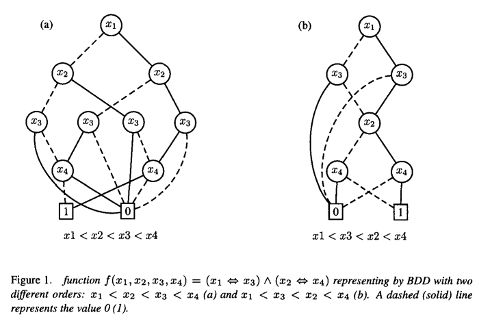
The size of a BDD structure (the number of nodes) depends critically on the chosen variable ordering. Figure 1 shows the effect of the variable ordering on the BDD size. If we consider the expression $\left(x_1 \Leftrightarrow x_3\right) \wedge\left(x_2 \Leftrightarrow x_4\right)$ the resulting BDD using the ordering $x_1<x_2<x_3<x_4$ consists of 11 nodes (figure 1(a)) and not 8 nodes as for the ordering $x_1<x_3<x_2<x_4$ (figure 1(b)). Finding an ordering that minimizes the size of BDD is also a NP-complete problem ${ }^7$. Several heuristics relying on different principles have been proposed in many domains. However, they both try to put close in the order the variables that are close in the formula as illustrated in figure 1 .

数学代写|运筹学作业代写operational research代考|Definitions and notations

The K-terminal reliability computation is the most general network reliability problem found in the literature. It consists in evaluating the probability that net work components of a specified subset $K$ remain connected when the components are subject to failure.

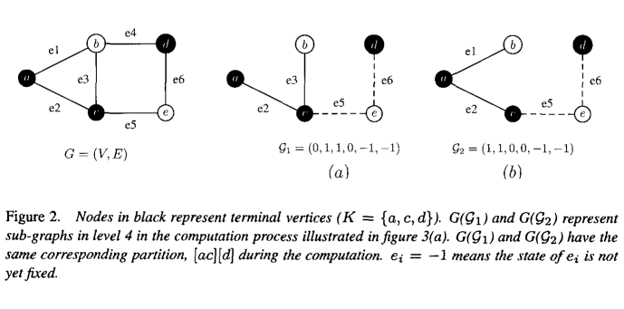
Our network model is an undirected stochastic graph $G=(V, E)$, with $V$ its set of vertex (representing workstations, servers, routers …) and $E \subseteq V \times V$ its set of edges (representing the links between these nodes). Each edge $e_i$ of the stochastic graph is subject to failure with known probability $q_i$. We denote $p_i=1-q_i$ the probability that edge $e_i$ functions, and assume that all the failure events are statistically independent. In the following, we consider the vertices as perfect, but the proposed algorithms are still functioning for such problem. In classical enumerative method, all the states of the graph are generated, evaluated as a fail state or a functioning state, and then probabilistic methods are used for computing the associated reliability. So, as there are two states for each edge, there are $2^m$ (with $m=|E|$ ) possible states for the graph. A state $\mathcal{G}$ of the stochastic graph $G$ is denoted by $\left(x_1, x_2 \ldots, x_m\right)$ where $x_i$ stands for the state of edge $e_i$, i.e. $x_i=0$ when edge $e_i$ fails and $x_i=1$ when it functions. The associated probability of $\mathcal{G}$ is defined as:
$$
\operatorname{Pr}(\mathcal{G})=\prod_{i=1}^m\left(x_i \cdot p_i+\left(1-x_i\right) \cdot q_i\right)
$$
At each state $\mathcal{G}$ is associated a partial graph $G(\mathcal{G})=\left(V, E^{\prime}\right)$ such that $e_i \in E^{\prime}$ if and only if $e_i \in E$ and $x_i=1$. A path is defined as a set of edges such that if these edges are all up, the system is up. A path is minimal if it has no proper subpaths. We define a subset of the nodes $K \subseteq V$ to be the “terminals” (with $2 \leq|K| \leq|V|)$. If $|K|=2$ this problem is well-known as the 2 -terminal reliability problem and if $|K|=|V|$ it deals with the all-terminal reliability problem. The terminal nodes are essential to the system function and have to communicate with each other, i.e. the network is up if and only if there exists at least one path made of functioning edges linking nodes in $K$. The K-terminal reliability, denoted by $R_K(p ; G)\left(p=\left(p_1, \ldots, p_m\right)\right)$, is the probability that all vertices in $K$ are connected and can be defined as follows:
$$
R_K(p ; G)=\sum_{\text {K-nodes are connected by working links in } G(\mathcal{G})} \operatorname{Pr}(\mathcal{G})
$$

运筹学代考

数学代写|运筹学作业代写operational research代考|Binary Decision Diagram (BDD)

Akers ${ }^1$首先引入BDD来表示布尔函数。Bryant通过引入一套有效构建和操作BDD结构${ }^2$的算法，推广了BDD的使用。目前，BDD已广泛应用于硬件综合与验证、模型检验和协议验证等领域。它们在可靠性分析框架中的使用已由Madre和Coudert ${ }^5 4$引入，并由Odeh ${ }^6$和Rauzy ${ }^3$开发。Sekine和Imai在网络可靠性方面引入了BDD结构${ }^{10} 11$。BDD结构提供了布尔表达式的紧凑表示。BDD是基于香农分解的有向无环图(DAG)。布尔函数$f$的香农分解定义如下:
$$
f=x f_{x=1}+\bar{x} f_{x=0}
$$
其中$x$是一个决策变量，$f_{x=i}$是布尔函数$f$，在$x=i$处求值。

该图有两个标记为0和1的汇聚节点，表示两个对应的常量表达式。每个内部节点都用布尔变量$x$标记，并有两个外边，分别称为0边和1边。1边连接的节点表示$x=1$时的布尔表达式，即$f_{x=1}$; 0边连接的节点表示$x=0$时的布尔表达式，即$f_{x=0}$。有序二进制决策图(OBDD)是一种BDD，其中变量根据已知的总排序排序，并且每个路径以升序访问变量。之后，bdd将被视为订购。BDD的叶节点为从根节点到叶节点的路径对应的赋值提供$f$。

BDD结构的大小(节点数量)主要取决于所选择的变量排序。图1显示了变量排序对BDD大小的影响。如果我们考虑表达式$\left(x_1 \Leftrightarrow x_3\right) \wedge\left(x_2 \Leftrightarrow x_4\right)$，那么使用顺序$x_1<x_2<x_3<x_4$得到的BDD由11个节点组成(图1(a))，而不是顺序$x_1<x_3<x_2<x_4$的8个节点(图1(b))。找到最小化BDD大小的排序也是一个np完全问题${ }^7$。许多领域都提出了基于不同原理的启发式方法。然而，它们都试图按照公式中接近的变量的顺序排列，如图1所示。

数学代写|运筹学作业代写operational research代考|Definitions and notations

k端可靠性计算是文献中发现的最普遍的网络可靠性问题。它包括评估特定子集$K$的网络组件在组件发生故障时保持连接的概率。

我们的网络模型是一个无向随机图$G=(V, E)$，其中$V$是一组顶点(代表工作站、服务器、路由器……)，$E \subseteq V \times V$是一组边(代表这些节点之间的链接)。随机图的每条边$e_i$都以已知的概率$q_i$失效。我们表示$p_i=1-q_i$边$e_i$函数的概率，并假设所有故障事件在统计上是独立的。在下面，我们认为顶点是完美的，但所提出的算法仍然适用于此类问题。在经典的枚举方法中，首先生成图的所有状态，并将其评估为失效状态或功能状态，然后使用概率方法计算相关的可靠度。因此，由于每条边都有两种状态，因此图有$2^m$(与$m=|E|$)可能的状态。随机图$G$的状态$\mathcal{G}$用$\left(x_1, x_2 \ldots, x_m\right)$表示，其中$x_i$表示边$e_i$的状态，即，当边$e_i$失效时为$x_i=0$，当边起作用时为$x_i=1$。$\mathcal{G}$的关联概率定义为:
$$
\operatorname{Pr}(\mathcal{G})=\prod_{i=1}^m\left(x_i \cdot p_i+\left(1-x_i\right) \cdot q_i\right)
$$
在每个状态$\mathcal{G}$都关联一个偏图$G(\mathcal{G})=\left(V, E^{\prime}\right)$，使得$e_i \in E^{\prime}$当且仅当$e_i \in E$和$x_i=1$。路径被定义为一组边，如果这些边都是上的，那么这个系统就是上的。如果一条路径没有合适的子路径，那么它就是最小路径。我们将节点的子集$K \subseteq V$定义为“终端”(使用$2 \leq|K| \leq|V|)$)。如果$|K|=2$这个问题是众所周知的2终端可靠性问题，如果$|K|=|V|$它处理的是全终端可靠性问题。终端节点对系统功能至关重要，并且必须相互通信，即当且仅当存在至少一条由连接$K$中的节点的功能边组成的路径时，网络才会启动。k端可靠度，用$R_K(p ; G)\left(p=\left(p_1, \ldots, p_m\right)\right)$表示，是$K$中所有顶点连通的概率，定义如下:
$$
R_K(p ; G)=\sum_{\text {K-nodes are connected by working links in } G(\mathcal{G})} \operatorname{Pr}(\mathcal{G})
$$

统计代写|运筹学作业代写operational research代考请认准statistics-lab™

统计代写请认准statistics-lab™. statistics-lab™为您的留学生涯保驾护航。

金融工程代写

金融工程是使用数学技术来解决金融问题。金融工程使用计算机科学、统计学、经济学和应用数学领域的工具和知识来解决当前的金融问题，以及设计新的和创新的金融产品。

非参数统计代写

非参数统计指的是一种统计方法，其中不假设数据来自于由少数参数决定的规定模型；这种模型的例子包括正态分布模型和线性回归模型。

广义线性模型代考

广义线性模型（GLM）归属统计学领域，是一种应用灵活的线性回归模型。该模型允许因变量的偏差分布有除了正态分布之外的其它分布。

术语广义线性模型（GLM）通常是指给定连续和/或分类预测因素的连续响应变量的常规线性回归模型。它包括多元线性回归，以及方差分析和方差分析（仅含固定效应）。

有限元方法代写

有限元方法（FEM）是一种流行的方法，用于数值解决工程和数学建模中出现的微分方程。典型的问题领域包括结构分析、传热、流体流动、质量运输和电磁势等传统领域。

有限元是一种通用的数值方法，用于解决两个或三个空间变量的偏微分方程（即一些边界值问题）。为了解决一个问题，有限元将一个大系统细分为更小、更简单的部分，称为有限元。这是通过在空间维度上的特定空间离散化来实现的，它是通过构建对象的网格来实现的：用于求解的数值域，它有有限数量的点。边界值问题的有限元方法表述最终导致一个代数方程组。该方法在域上对未知函数进行逼近。[1] 然后将模拟这些有限元的简单方程组合成一个更大的方程系统，以模拟整个问题。然后，有限元通过变化微积分使相关的误差函数最小化来逼近一个解决方案。

tatistics-lab作为专业的留学生服务机构，多年来已为美国、英国、加拿大、澳洲等留学热门地的学生提供专业的学术服务，包括但不限于Essay代写，Assignment代写，Dissertation代写，Report代写，小组作业代写，Proposal代写，Paper代写，Presentation代写，计算机作业代写，论文修改和润色，网课代做，exam代考等等。写作范围涵盖高中，本科，研究生等海外留学全阶段，辐射金融，经济学，会计学，审计学，管理学等全球99%专业科目。写作团队既有专业英语母语作者，也有海外名校硕博留学生，每位写作老师都拥有过硬的语言能力，专业的学科背景和学术写作经验。我们承诺100%原创，100%专业，100%准时，100%满意。

随机分析代写

随机微积分是数学的一个分支，对随机过程进行操作。它允许为随机过程的积分定义一个关于随机过程的一致的积分理论。这个领域是由日本数学家伊藤清在第二次世界大战期间创建并开始的。

时间序列分析代写

随机过程，是依赖于参数的一组随机变量的全体，参数通常是时间。随机变量是随机现象的数量表现，其时间序列是一组按照时间发生先后顺序进行排列的数据点序列。通常一组时间序列的时间间隔为一恒定值（如1秒，5分钟，12小时，7天，1年），因此时间序列可以作为离散时间数据进行分析处理。研究时间序列数据的意义在于现实中，往往需要研究某个事物其随时间发展变化的规律。这就需要通过研究该事物过去发展的历史记录，以得到其自身发展的规律。

回归分析代写

多元回归分析渐进（Multiple Regression Analysis Asymptotics）属于计量经济学领域，主要是一种数学上的统计分析方法，可以分析复杂情况下各影响因素的数学关系，在自然科学、社会和经济学等多个领域内应用广泛。

MATLAB代写

MATLAB 是一种用于技术计算的高性能语言。它将计算、可视化和编程集成在一个易于使用的环境中，其中问题和解决方案以熟悉的数学符号表示。典型用途包括：数学和计算算法开发建模、仿真和原型制作数据分析、探索和可视化科学和工程图形应用程序开发，包括图形用户界面构建MATLAB 是一个交互式系统，其基本数据元素是一个不需要维度的数组。这使您可以解决许多技术计算问题，尤其是那些具有矩阵和向量公式的问题，而只需用 C 或 Fortran 等标量非交互式语言编写程序所需的时间的一小部分。MATLAB 名称代表矩阵实验室。MATLAB 最初的编写目的是提供对由 LINPACK 和 EISPACK 项目开发的矩阵软件的轻松访问，这两个项目共同代表了矩阵计算软件的最新技术。MATLAB 经过多年的发展，得到了许多用户的投入。在大学环境中，它是数学、工程和科学入门和高级课程的标准教学工具。在工业领域，MATLAB 是高效研究、开发和分析的首选工具。MATLAB 具有一系列称为工具箱的特定于应用程序的解决方案。对于大多数 MATLAB 用户来说非常重要，工具箱允许您学习和应用专业技术。工具箱是 MATLAB 函数（M 文件）的综合集合，可扩展 MATLAB 环境以解决特定类别的问题。可用工具箱的领域包括信号处理、控制系统、神经网络、模糊逻辑、小波、仿真等。

R语言代写	问卷设计与分析代写
PYTHON代写	回归分析与线性模型代写
MATLAB代写	方差分析与试验设计代写
STATA代写	机器学习/统计学习代写
SPSS代写	计量经济学代写
EVIEWS代写	时间序列分析代写
EXCEL代写	深度学习代写
SQL代写	各种数据建模与可视化代写

数学代写|运筹学作业代写operational research代考|MATH3901

Posted on 2023年8月23日2023年8月23日 by statistics-lab

数学代写|运筹学作业代写operational research代考|The Markov Chain Monte Carlo Method

In this section, we present the utilisation of Markov chain Monte Carlo method (see Chen, Shao and Ibrahim $^6$ ) for estimating $\tau$ and the parameters of the initial lifetime distribution. To simplify the matter, we assume that the first two lifetimes are observed and the repair type is known to be WTNBTU.

The McMC methods enable us to simulate a Markov chain whose stationary distribution is our “target” distribution, for instance, the posterior distribution of the parameter of interest. We will use the Gibbs sampler which is one of the McMC methods. Under our model, the Gibbs sampler can be described as follows:
(1) Start with an arbitrary initial vector $\theta^{(0)}=\left(\tau^{(0)}, \alpha^{(0)}, \beta^{(0)}\right)$ and set $k=0$.
(2) Sample $\tau^{(k+1)}$ from $\pi\left(\tau \mid \alpha^{(k)}, \beta^{(k)}, x_1, x_2\right)$.
(3) Sample $\alpha^{(k+1)}$ from $\pi\left(\alpha \mid \tau^{(k+1)}, \beta^{(k)}, x_1, x_2\right)$.
(4) Sample $\beta^{(k+1)}$ from $\pi\left(\beta \mid \tau^{(k+1)}, \alpha^{(k+1)}, x_1, x_2\right)$.
(5) Set $\theta^{(k+1)}=\left(\tau^{(k+1)}, \alpha^{(k+1)}, \beta^{(k+1)}\right)$ and $k=k+1$. Go back to the second step.

Here, $\pi(\cdot \mid \cdot)$ denotes a full conditional density function. For instance,
$$
\pi\left(\tau \mid \alpha^{(k)}, \beta^{(k)}, x_1, x_2\right)
$$

denotes the conditional density function of $\tau$ given current values of all the other parameters as well as two failure times. One can obtain each full conditional density up to a proportionality constant as follows by, firstly, obtaining the joint density function of all the parameters and failure times, i.e.,
$$
L\left(\tau, \alpha, \beta \mid x_1, x_2\right) \pi(\tau) \pi(\alpha) \pi(\beta),
$$
and then viewing (5) as a function of the parameter of interest. With our model assumptions, direct sampling from each full conditional cannot be easily done due to the indexing parameter $\tau$ (see Gilks ${ }^5$ ). MetropolisHastings algorithms (see Metropolis et al. ${ }^8$ and Hastings ${ }^9$ ) can be used to draw samples from the full conditionals. The Metropolis-Hastings method is an McMC methods that includes the Gibbs sampler as a special case (see Chib and Greenberg $\left.{ }^7\right)$. Under certain regularity conditions, for sufficiently large $k,\left{\theta^{(m)}: k \leq m \leq(k+n-1)\right}$ is approximately an i.i.d. sample of size $n$ from the posterior distribution of $\tau, \alpha, \beta$ given $\left(x_1, x_2\right)$. Numerical examples will illustrate our approach.

数学代写|运筹学作业代写operational research代考|Example

In this section we will reconsider the example discussed in ${ }^{12}$ and summarize the findings on the estimation of $\tau$ using maximum likelihood approach. Further, we will estimate $\tau$ from Bayesian prospective and compare the results of the two approaches. As in ${ }^{12}$, we will restrict our attention on the comparison of two consecutive lifetime distributions by using corresponding failure rate functions.
We will begin with the following assumptions:

The item, $S$, subject to failures/repairs, has a complex structure comprising $m$ subsystems, i.e., $S=\left{S_1, S_2, \ldots S_m\right}$.
A failure of a particular subsystem requires a type of repair which is known in advance.

For example, let us consider a car. If the failure affects the tires of a car (say subsystem $S_1$ ), usually a complete repair is required. On the other hand, if the charging system of the car (say subsystem $S_2$ ) fails, worse than new, better than used (WTNBTU) repair is performed. The information on warranty failures and repairs is usually strictly confidential and it is very difficult to obtain real warranty data even for research purposes. For this reason we demonstrate how one might estimate the parameters of our model using simulated data.

运筹学代考

数学代写|运筹学作业代写operational research代考|The Markov Chain Monte Carlo Method

在本节中，我们提出利用马尔可夫链蒙特卡罗方法(见Chen, Shao和Ibrahim $^6$)来估计$\tau$和初始寿命分布的参数。为了简化问题，我们假设观察到前两个生命周期，并且已知修复类型为WTNBTU。

McMC方法使我们能够模拟一个马尔可夫链，其平稳分布是我们的“目标”分布，例如，感兴趣的参数的后验分布。我们将使用Gibbs采样器，这是McMC方法之一。在我们的模型下，吉布斯采样器可以描述为:
(1)从任意初始向量$\theta^{(0)}=\left(\tau^{(0)}, \alpha^{(0)}, \beta^{(0)}\right)$开始，设置$k=0$。
(2)样本$\tau^{(k+1)}$来自$\pi\left(\tau \mid \alpha^{(k)}, \beta^{(k)}, x_1, x_2\right)$。
(3)从$\pi\left(\alpha \mid \tau^{(k+1)}, \beta^{(k)}, x_1, x_2\right)$获取$\alpha^{(k+1)}$样本。
(4)从$\pi\left(\beta \mid \tau^{(k+1)}, \alpha^{(k+1)}, x_1, x_2\right)$获取$\beta^{(k+1)}$样本。
(5)设置$\theta^{(k+1)}=\left(\tau^{(k+1)}, \alpha^{(k+1)}, \beta^{(k+1)}\right)$和$k=k+1$。回到第二步。

这里，$\pi(\cdot \mid \cdot)$表示一个完整的条件密度函数。例如，
$$
\pi\left(\tau \mid \alpha^{(k)}, \beta^{(k)}, x_1, x_2\right)
$$

表示在给定所有其他参数的电流值和两次失效次数时$\tau$的条件密度函数。我们可以得到每一个达到比例常数的满条件密度，方法如下:首先，得到所有参数和失效时间的联合密度函数，即
$$
L\left(\tau, \alpha, \beta \mid x_1, x_2\right) \pi(\tau) \pi(\alpha) \pi(\beta),
$$
然后将(5)作为感兴趣参数的函数。使用我们的模型假设，由于索引参数$\tau$(参见Gilks ${ }^5$)，从每个完整条件中直接抽样不容易完成。MetropolisHastings算法(参见Metropolis等人${ }^8$和Hastings ${ }^9$)可用于从完整条件中提取样本。Metropolis-Hastings方法是一种McMC方法，其中包括吉布斯采样器作为一种特殊情况(参见Chib和Greenberg $\left.{ }^7\right)$)。在一定的正则性条件下，对于足够大的$k,\left{\theta^{(m)}: k \leq m \leq(k+n-1)\right}$近似为一个大小为$n$的i.i.d样本，来自于$\tau, \alpha, \beta$给定$\left(x_1, x_2\right)$的后验分布。数值例子将说明我们的方法。

数学代写|运筹学作业代写operational research代考|Example

在本节中，我们将重新考虑${ }^{12}$中讨论的示例，并总结使用最大似然方法估计$\tau$的结果。进一步，我们将从贝叶斯的角度估计$\tau$，并比较两种方法的结果。与${ }^{12}$一样，我们将通过使用相应的故障率函数将注意力限制在两个连续寿命分布的比较上。
我们将从以下假设开始:

项目$S$有故障/修理，结构复杂，包括$m$个子系统，即$S=\left{S_1, S_2, \ldots S_m\right}$。

一个特定子系统的故障需要一种预先知道的修复方法。

例如，让我们考虑一辆汽车。如果故障影响到汽车的轮胎(比如子系统$S_1$)，通常需要进行彻底的修理。另一方面，如果汽车的充电系统(例如子系统$S_2$)发生故障，则进行比新更坏，比旧更好(WTNBTU)的维修。关于保修故障和维修的信息通常是严格保密的，即使是为了研究目的，也很难获得真实的保修数据。出于这个原因，我们演示了如何使用模拟数据估计模型的参数。

统计代写请认准statistics-lab™. statistics-lab™为您的留学生涯保驾护航。

金融工程代写

非参数统计代写

非参数统计指的是一种统计方法，其中不假设数据来自于由少数参数决定的规定模型；这种模型的例子包括正态分布模型和线性回归模型。

广义线性模型代考

广义线性模型（GLM）归属统计学领域，是一种应用灵活的线性回归模型。该模型允许因变量的偏差分布有除了正态分布之外的其它分布。

有限元方法代写

随机分析代写

时间序列分析代写

回归分析代写

MATLAB代写

R语言代写	问卷设计与分析代写
PYTHON代写	回归分析与线性模型代写
MATLAB代写	方差分析与试验设计代写
STATA代写	机器学习/统计学习代写
SPSS代写	计量经济学代写
EVIEWS代写	时间序列分析代写
EXCEL代写	深度学习代写
SQL代写	各种数据建模与可视化代写

数学代写|数学建模代写math modelling代考|MATH4413

Posted on 2023年8月21日2023年10月10日 by statistics-lab

如果你也在怎样代写数学建模Mathematical Modeling这个学科遇到相关的难题，请随时右上角联系我们的24/7代写客服。数学建模Mathematical Modeling最好是通过制作数学模型来学习的。为实现这一目标，已编制了三种类型的演习。其中一些进一步发展了文中给出的模型;另一些要求读者改变文中给出的模型的假设，然后，推断新模型的结果，并与新情况的结果进行比较。

数学建模Mathematical Modeling都是从物理、生物、社会、经济、管理和工程科学中选择的。这些模型处理不同的概念，但具有共同的数学结构，并体现了不同学科数学建模的统一影响。因此，物理学、生物学、经济学、心理学和工程学中完全不同的问题可以用一个共同的数学模型来表示。模型是一样的;只是解释不同而已。当不同的技术是最合适的时候，努力解释概念。

statistics-lab™ 为您的留学生涯保驾护航在代写数学建模math modelling方面已经树立了自己的口碑, 保证靠谱, 高质且原创的统计Statistics代写服务。我们的专家在代写数学建模math modelling代写方面经验极为丰富，各种代写数学建模math modelling相关的作业也就用不着说。

数学代写|数学建模代写math modelling代考|Bifurcation Analysis and Open-Loop Stability

To find suitable operational regions of the $\mathrm{ABE}$ process, a bifurcation analysis was performed. Figures 2(a-c) show the bifurcation diagrams (at steady state) for biomass, glycerol and butanol, employing the dilution rate and the glycerol inlet concentration as bifurcation parameters. The figures show that when a glycerol inlet concentration close to $60 \mathrm{~g} \mathrm{~L}^{-1}$ and a dilution rate value of $0.062 \mathrm{~h}^{-1}$, it is possible to obtain a glycerol consumption of $97.5 \%$. It can be noted that under these conditions, biomass concentrations close to $30 \mathrm{~g} \mathrm{~L}^{-1}$ and a production of butanol of 9.4 $\mathrm{g} \mathrm{L}^{-1}$ can be obtained, this is a natural response of the fermentation, such that with an increase of the corresponding substrate the biomass growth is also increased, improving the butanol generation, under the restrictiction of the inhibitory substrate concentration value. From this analysis, it was observed that the butanol concentration can be increased up to $62 \%$. Similar operating conditions near to this operational region can be selected as suitable operating set points for controlling purposes. For our case study, $8 \mathrm{~g} \mathrm{~L}^{-1}$ and $9.4 \mathrm{~g} \mathrm{~L}^{-1}$ of butanol were selected as reference points. Can be noticed that with the bifurcation analysis the rank of the dilituin rate can also be determinated, is observed that higher values of the dilution rate, the residence time of the reactives in the bioreactor is diminished together with the glycerol conversion.

Moreover, it is widely known that an equilibrium point of the dynamic system is stable if all the eigenvalues $(\lambda)$ have negative real parts of their linear representation by the Jacobian matrix of the system. An equilibrium point is unstable if at least one of the eigenvalues has a positive real part [31]. The eigenvalues corresponding to the equilibrium points of biomass, glycerol and butanol presented in Figures 1(a-c), resulted for all cases with negative real values (data not shown), which indicates that the equilibrium points presented from this analysis are stable, under the selected operation conditions. However, under small changes of process parameters the corresponding equilibrium points can be altered, leading the bioreactor production to undesirable process conditions, such as washout regimen, low conversion regimen, input multiplicity and so on.

数学代写|数学建模代写math modelling代考|Closed Loop Analysis

Numerical experiments were carried out to show the closed-loop behavior of the bioreactor. The initial conditions were $x_l=0.05 \mathrm{~g} \mathrm{~L}^{-1}, x_2=40 \mathrm{~g} \mathrm{~L}^{-1}$, $x_3=0.0 \mathrm{~g} \mathrm{~L}^{-1}$ and $x_{2 i n}=60 \mathrm{~g} \mathrm{~L}^{-1}$. The proposed controller is based on a single input-single output (SISO) structure, where the butanol concentration is considered as the controlled variable, while the input flow defined by the dilution rate $(D)$, is considered as the control input. The controller parameters were estimated as $k_l=300 \mathrm{~g}^3 \mathrm{~L}^{-3}$ and $k_2=0.016 \mathrm{~h}^{-1}$ in accordance with the previous theoretical results. The parameter $n$ obeys the theoretical property given by the inequality of Eq. (11), but for practical application $n=3$ is proposed, resulting in a cubic controller. The $n$ value was selected considering the best output control response and the corresponding control effort. Furthermore, numerical experiments were programmed so that after $60 \mathrm{~h}$ the control law is activated with a first set point of $x_{3 s p}=8 \mathrm{gL}^{-1}$. Subsequently, after $100 \mathrm{~h}$, a second set point, $x_{3 s p}=$ $9.4 \mathrm{gL}^{-1}$ is activated. It is important to note that the selected set points are in accordance with the results from the bifurcation analysis, in order to select operating points with a high butanol production and avoid the inhibition effect. As mentioned, the control task is the increase of the butanol concentration via the dilution rate manipulation via the proposed control law. However, as can be observed in the mathematical model structure of the bioreactor, the dilution rate affect to all the state equations and then their corresponding dynamic response, for this is necessary to analyse the dynamic response of the properly uncontrolled variables under variation of the dilution rate to prevent undesirable effects or unstabilities of this uncontrolled mass concentrations. The above mentioned undesirable effects can include inhibitory glycerol concentrations and biomass washout in the bioreactor.

数学建模代写

数学代写|数学建模代写math modelling代考|Bifurcation Analysis and Open-Loop Stability

为了找到$\ mathm {ABE}$过程的合适操作区域，进行了分岔分析。图2(a-c)显示了生物质、甘油和丁醇的分岔图(稳态)，分岔参数为稀释率和甘油进口浓度。由图可知，当甘油进口浓度接近$60 \ mathm {~g} \ mathm {~L}^{-1}$，稀释率值为$0.062 \ mathm {~h}^{-1}$时，甘油消耗量可达$ 97.5% $。可以注意到，在这些条件下，可以获得接近$30 \ mathm {~g} \ mathm {~L}^{-1}$的生物量浓度和9.4 $\ mathm {g} \ mathm {L}^{-1}$的丁醇产量，这是发酵的自然反应，在抑制底物浓度值的限制下，随着相应底物的增加，生物量的增长也随之增加，提高了丁醇的生成。从这个分析中可以看出，丁醇的浓度可以提高到62%。在该操作区域附近，可以选择类似的操作条件作为合适的操作设定点进行控制。选取$8 \mathrm{~g} \mathrm{~L}^{-1}$和$9.4 \mathrm{~g} \mathrm{~L}^{-1}$作为丁醇的参考点。可以注意到，通过分岔分析，还可以确定稀释率的等级，观察到稀释率值越高，反应物在生物反应器中的停留时间越短，甘油转化率也越低。

此外，众所周知，如果系统的雅可比矩阵表示的所有特征值$(\ λ)$的线性表示具有负实部，则动态系统的平衡点是稳定的。如果至少有一个特征值具有正实部，则平衡点是不稳定的[31]。图1(a-c)所示的生物质、甘油和丁醇的平衡点对应的特征值在所有实值为负的情况下(数据未显示)都得到，这表明在所选的操作条件下，本分析给出的平衡点是稳定的。然而，在工艺参数的微小变化下，相应的平衡点可能发生改变，导致生物反应器生产出现不良的工艺条件，如冲洗工况、低转化率工况、输入多重性等。

数学代写|数学建模代写math modelling代考|Closed Loop Analysis

通过数值实验验证了生物反应器的闭环特性。初始条件x_l = 0.05美元\ mathrm {~ g} \ mathrm {~ L} ^ {1}, x_2 = 40 \ mathrm {~ g} \ mathrm {~ L} ^ {1} $, x_3 = 0.0美元\ mathrm {~ g} \ mathrm {~ L} ^{1}和美元间的{2 i n} = 60 \ mathrm {~ g} \ mathrm {~ L} ^{1} $。所提出的控制器基于单输入-单输出(SISO)结构，其中丁醇浓度被认为是受控变量，而稀释率$(D)$定义的输入流量被认为是控制输入。根据前人的理论结果，估计控制器参数为$k_l=300 \ mathm {~g}^3 \ mathm {~L}^{-3}$和$k_2=0.016 \ mathm {~h}^{-1}$。参数$n$符合公式(11)不等式的理论性质，但在实际应用中，我们提出$n=3$，从而得到一个三次控制器。考虑最佳输出控制响应和相应的控制努力，选择$n$值。在$60 \ mathm {~h}$后，以$x_{3 s p}=8 \ mathm {gL}^{-1}$为第一个设定点激活控制律。随后，在$100 \mathrm{~h}$之后，第二个设定点$x_{3 s p}=$ $9.4 \mathrm{gL}^{-1}$被激活。重要的是要注意，所选择的设定值与分岔分析的结果一致，以便选择具有高丁醇产量的操作点并避免抑制效应。如前所述，控制任务是通过提出的控制律通过稀释率操作来增加丁醇浓度。然而，从生物反应器的数学模型结构中可以看出，稀释率会影响所有状态方程，进而影响它们相应的动态响应，因此有必要分析适当的不受控制变量在稀释率变化下的动态响应，以防止这种不受控制的质量浓度产生不良影响或不稳定。上述不良影响可包括生物反应器中的抑制甘油浓度和生物质冲洗。

数学代写|数学建模代写math modelling代考请认准statistics-lab™

统计代写请认准statistics-lab™. statistics-lab™为您的留学生涯保驾护航。

金融工程代写

非参数统计代写

非参数统计指的是一种统计方法，其中不假设数据来自于由少数参数决定的规定模型；这种模型的例子包括正态分布模型和线性回归模型。

广义线性模型代考

广义线性模型（GLM）归属统计学领域，是一种应用灵活的线性回归模型。该模型允许因变量的偏差分布有除了正态分布之外的其它分布。

有限元方法代写

随机分析代写

时间序列分析代写

回归分析代写

MATLAB代写

R语言代写	问卷设计与分析代写
PYTHON代写	回归分析与线性模型代写
MATLAB代写	方差分析与试验设计代写
STATA代写	机器学习/统计学习代写
SPSS代写	计量经济学代写
EVIEWS代写	时间序列分析代写
EXCEL代写	深度学习代写
SQL代写	各种数据建模与可视化代写

数学代写|数学建模代写math modelling代考|MATH1800

Posted on 2023年8月21日2023年8月28日 by statistics-lab

数学代写|数学建模代写math modelling代考|Basic Reproduction Number

The basic reproduction number $R_0$ is the potential measurement for spreading disease in a population. Mathematically, $R_0$ is a threshold parameter for the stability of a disease-free equilibrium and is related to the peak and final density of an epidemic. It is defined as the expected number of secondary cases of infection which would occur due to a primary case in a completely susceptible population [26]. If $R_0<1$, then a few infected individuals introduced into a completely susceptible population will, on average, fail to replace themselves, and the disease will not spread. On the other hand, when $R_0>1$, then the number of infected individuals will increase with each generation and the disease will spread. Moreover, it is noted that the basic reproduction number is a threshold parameter for invasion of a disease organism into a completely susceptible population; if the disease begins to spread, conditions favoring spread will change and $R_0$ may no longer be a good measure of disease transmission. However, in many disease transmission models, the peak prevalence of infected hosts and the final size of the epidemic are increasing functions of $R_0$, making it a useful measure of spread.

Now, according to the biological interpretation, we can define the basic reproduction number We can define the basic reproduction number $R_0$ by the method of next generation matrix method [27] in the following form
$$
R_0=\beta \times \frac{\alpha}{\alpha+\varepsilon_1+\mu} \times \frac{1}{\delta+\varepsilon_2+\mu},
$$
where $\frac{\alpha}{\alpha+\varepsilon_1+\mu}$ is the probability that an individual has become infectious (moved from $E$ to $I$ ), and $\frac{1}{\delta+\varepsilon_2+\mu}$ is the average time that a person is infectious (spends in $I$ class). The equation (6) can be rewritten as the following form
$$
R_0=\frac{\alpha \beta}{\phi_1 \phi_2},
$$
where $\phi_1=\alpha+\varepsilon_1+\mu$ and $\phi_2=\delta+\varepsilon_2+\mu$.

数学代写|数学建模代写math modelling代考|Equilibrium Analysis

In this section, we investigate the existence of non-negative equilibria of the system (1) by solving the following nonlinear algebraic system
$$
\left{\begin{array}{l}
\Lambda-\beta I S-\mu S=0, \
(1-p) \beta I S-\phi_1 E=0, \
p \beta I S+\alpha E-\phi_2 I=0, \
\varepsilon_1 E+\varepsilon_2 I-\mu R=0 .
\end{array}\right.
$$
By solving the system (8), we find the following two non-negative equilibria of the model (1) only: one is disease-free equilibrium $E_1$ and other one is endemic equilibrium $E_$, where $\phi_1=\alpha+\mu+\varepsilon_1$ and $\phi_2=\delta+\mu+\varepsilon_2$, $$ E_1\left(\frac{\Lambda}{\mu}, 0,0,0\right) \text {, and } E_\left(S^, E^, I^, R^\right),
$$

where
$$
\begin{aligned}
S^* & =\frac{\phi_1 \phi_2}{\alpha \beta(1-p)+p \beta \phi_1}, E^=\frac{(1-p)\left(\Lambda \alpha \beta(1-p)+p \beta \Lambda \phi_1-\mu \phi_1 \phi_2\right)}{\alpha \beta \phi_1(1-p)+p \beta \phi_1^2}, \ I^ & =\frac{\left(\Lambda \alpha \beta(1-p)+p \beta \Lambda \phi_1-\mu \phi_1 \phi_2\right)}{\beta \phi_1 \phi_2}, \
R^* & =\frac{\left(\alpha \varepsilon_2(1-p)+\varepsilon_1 \phi_2(1-p)+p \varepsilon_2 \phi_1\right)\left(\Lambda \alpha \beta(1-p)+p \beta \Lambda \phi_1-\mu \phi_1 \phi_2\right)}{\alpha \beta \mu \phi_1(1-p)+p \mu \beta \phi_1^2 \phi_2} .
\end{aligned}
$$
The semitrivial equilibria $E_1$ always exist while the nontrivial equilibrium point $E_*$ exists underlying the condition $\Lambda \alpha \beta(1-p)+p \beta \Lambda \phi_1>\mu \phi_1 \phi_2$.
A local stability analysis of the system (2) is performed around the equilibria presented in the previous section. To do so, we linearize the system (1) around the equilibrium point $(\bar{S}, \bar{E}, \bar{I}, \bar{R})$ so that the following Jacobian matrix can be obtained
$$
J(\bar{S}, \bar{E}, \bar{I}, \bar{R})=\left[\begin{array}{cccc}
-(\beta \bar{I}+\mu) & 0 & -\beta \bar{S} & 0 \
(1-p) \beta \bar{I} & -\phi_1 & (1-p) \beta \bar{S} & 0 \
p \beta \bar{I} & \alpha & p \beta \bar{S}-\phi_2 & 0 \
0 & \varepsilon_1 & \varepsilon_2 & -\mu
\end{array}\right]
$$

数学建模代写

数学代写|数学建模代写math modelling代考|Basic Reproduction Number

基本繁殖数$R_0$是衡量疾病在人群中传播的潜在指标。在数学上，$R_0$是无病平衡稳定性的阈值参数，与流行病的峰值和最终密度有关。它被定义为在完全易感人群中因原发病例而发生的继发病例的预期数量[26]。如果$R_0<1$，那么一些被感染的个体被引入到一个完全易感的群体中，平均来说，将无法自我替换，疾病将不会传播。另一方面，当$R_0>1$时，那么感染个体的数量将随着每一代的增加而增加，疾病将会传播。此外，还应指出，基本繁殖数是疾病生物体侵入完全易感群体的阈值参数;如果疾病开始传播，有利于传播的条件将发生变化，$R_0$可能不再是疾病传播的良好衡量标准。然而，在许多疾病传播模型中，受感染宿主的峰值流行率和流行病的最终规模增加了$R_0$的函数，使其成为有用的传播度量。

现在，根据生物学的解释，我们可以定义基本繁殖数，我们可以用下一代矩阵法[27]的方法定义基本繁殖数$R_0$，形式如下
$$
R_0=\beta \times \frac{\alpha}{\alpha+\varepsilon_1+\mu} \times \frac{1}{\delta+\varepsilon_2+\mu},
$$
其中$\frac{\alpha}{\alpha+\varepsilon_1+\mu}$是个体具有传染性的概率(从$E$转移到$I$)， $\frac{1}{\delta+\varepsilon_2+\mu}$是一个人具有传染性的平均时间(在$I$课上花费的时间)。式(6)可改写为如下形式
$$
R_0=\frac{\alpha \beta}{\phi_1 \phi_2},
$$
其中$\phi_1=\alpha+\varepsilon_1+\mu$和$\phi_2=\delta+\varepsilon_2+\mu$。

数学代写|数学建模代写math modelling代考|Equilibrium Analysis

在本节中，我们通过求解以下非线性代数系统来研究系统(1)的非负平衡点的存在性
$$
\left{\begin{array}{l}
\Lambda-\beta I S-\mu S=0, \
(1-p) \beta I S-\phi_1 E=0, \
p \beta I S+\alpha E-\phi_2 I=0, \
\varepsilon_1 E+\varepsilon_2 I-\mu R=0 .
\end{array}\right.
$$
通过求解系统(8)，我们发现模型(1)只有以下两个非负均衡:一个是无病均衡$E_1$，另一个是地方病均衡$E_$，其中$\phi_1=\alpha+\mu+\varepsilon_1$和$\phi_2=\delta+\mu+\varepsilon_2$， $$ E_1\left(\frac{\Lambda}{\mu}, 0,0,0\right) \text {, and } E_\left(S^, E^, I^, R^\right),
$$

在哪里
$$
\begin{aligned}
S^* & =\frac{\phi_1 \phi_2}{\alpha \beta(1-p)+p \beta \phi_1}, E^=\frac{(1-p)\left(\Lambda \alpha \beta(1-p)+p \beta \Lambda \phi_1-\mu \phi_1 \phi_2\right)}{\alpha \beta \phi_1(1-p)+p \beta \phi_1^2}, \ I^ & =\frac{\left(\Lambda \alpha \beta(1-p)+p \beta \Lambda \phi_1-\mu \phi_1 \phi_2\right)}{\beta \phi_1 \phi_2}, \
R^* & =\frac{\left(\alpha \varepsilon_2(1-p)+\varepsilon_1 \phi_2(1-p)+p \varepsilon_2 \phi_1\right)\left(\Lambda \alpha \beta(1-p)+p \beta \Lambda \phi_1-\mu \phi_1 \phi_2\right)}{\alpha \beta \mu \phi_1(1-p)+p \mu \beta \phi_1^2 \phi_2} .
\end{aligned}
$$
半平凡平衡点$E_1$总是存在，而非平凡平衡点$E_*$在条件$\Lambda \alpha \beta(1-p)+p \beta \Lambda \phi_1>\mu \phi_1 \phi_2$下存在。
系统(2)的局部稳定性分析是围绕前一节中提出的平衡点进行的。为此，我们围绕平衡点$(\bar{S}, \bar{E}, \bar{I}, \bar{R})$对系统(1)进行线性化，从而可以得到下面的雅可比矩阵
$$
J(\bar{S}, \bar{E}, \bar{I}, \bar{R})=\left[\begin{array}{cccc}
-(\beta \bar{I}+\mu) & 0 & -\beta \bar{S} & 0 \
(1-p) \beta \bar{I} & -\phi_1 & (1-p) \beta \bar{S} & 0 \
p \beta \bar{I} & \alpha & p \beta \bar{S}-\phi_2 & 0 \
0 & \varepsilon_1 & \varepsilon_2 & -\mu
\end{array}\right]

统计代写请认准statistics-lab™. statistics-lab™为您的留学生涯保驾护航。

金融工程代写

非参数统计代写

非参数统计指的是一种统计方法，其中不假设数据来自于由少数参数决定的规定模型；这种模型的例子包括正态分布模型和线性回归模型。

广义线性模型代考

广义线性模型（GLM）归属统计学领域，是一种应用灵活的线性回归模型。该模型允许因变量的偏差分布有除了正态分布之外的其它分布。

有限元方法代写

随机分析代写

时间序列分析代写

回归分析代写

MATLAB代写

R语言代写	问卷设计与分析代写
PYTHON代写	回归分析与线性模型代写
MATLAB代写	方差分析与试验设计代写
STATA代写	机器学习/统计学习代写
SPSS代写	计量经济学代写
EVIEWS代写	时间序列分析代写
EXCEL代写	深度学习代写
SQL代写	各种数据建模与可视化代写

数学代写|数学建模代写math modelling代考|MATH3041

Posted on 2023年8月21日2023年8月21日 by statistics-lab

数学代写|数学建模代写math modelling代考|Mathematical Modeling of Solving the Combinatorial Tasks of Minimizing Costs in the Process of Creating High-Tech Digital Production Structures

In modern conditions, one of the most significant functional strategies of an enterprise becomes an innovative component of the competitive strategy (Radiyevsky, 2013). In the process of innovation activity, enterprises create production systems focused on flexible automation and the use of innovative technologies (process innovations) and produce competitive products on the global market. This strategy leads to the emergence of an innovation subsystem that dominates the management system. This subsystem is based on technological innovations that generate organizational and managerial, resource, financial, economic and other types of innovations (Baranov et al., 2016).

The process innovations created by an enterprise, which take the form of technological capital, give an impulse for further development of innovative processes, in particular, the processes of formation of high-tech robotic organizational and production structures (Nikolaev et al., 2010). This leads to the appearance of not only modern highly automated fixed assets, but also organizational and managerial innovations, existing as a set of mathematical models, methods and information tools for building highly automated structures (Baranov et al., 2016).

Thus, technological capital generates the ability of an enterprise to use rational ways of organizing production processes based on the optimal combination of various components of capital (financial, intellectual, etc.) (Fatkhutdinov, 2015; Shishmarev, 2015). In its turn, technological capital, acting in the form of various intellectual property objects (patented technologies, unique know-hows, etc.), activates organizational and economic relations, both at the level of the enterprise as a whole and at the level of its individual structural components (Baranov et al., 2016).

Given the importance of the innovation subsystem and its technological capital for the competitiveness of the enterprise, the task of modeling the optimal composition of production units of high-tech organizational and production structures arises (Struchenkov, 2016). The formation of such units presupposes the introduction of highly automated equipment and industrial robots into their composition, which performs the functions of transport and transfer devices.

数学代写|数学建模代写math modelling代考|Results and Discussion

The set of dynamic models proposed in the chapter provides for the economically reasonable selection of the best alternative to create high-tech digital structures at the enterprise level. The models include a compact description of interaction between the innovative modernization factors affecting the adoption of the optimal decision. The resulting set of models is combined, as it deploys integer variables along with continuous parameters and the model limits are of the nonlinear form. The developed modifications of the economic mathematical model enable the enterprise to reduce costs on the design of high-tech structures at the set values of the production program or the automation level of the technological equipment.

The discrete programming task related to the development of the optimal program of the high-tech production structures has been solved within the modeling process of the production capacity management strategy. The analysis of various heuristic algorithms allowed substantiating the selection of the algorithm built on the Johnson method. The developed model was used to solve the selection problem of the optimal ratio between the flexibility and productivity of high-tech production structures.

For highly automated organizational and production structures of hightech enterprises the task was solved for the management of their production capacity mastering processes. Mastering of the production capacities was described as a transient process by an inhomogeneous difference equation. The integral solution was presented as a sum of the global solution of the homogeneous equation and the particular solution of the inhomogeneous equation. Layout implementation of the problem solution model and algorithm in a high-level programming language demonstrated high robustness of this model, allowing the reduction of requirements applied to the quality of source data.

数学建模代写

数学代写|数学建模代写math modelling代考|Mathematical Modeling of Solving the Combinatorial Tasks of Minimizing Costs in the Process of Creating High-Tech Digital Production Structures

在现代条件下，企业最重要的功能战略之一成为竞争战略的创新组成部分(Radiyevsky, 2013)。在创新活动的过程中，企业创造了以灵活自动化和使用创新技术(工艺创新)为重点的生产系统，并生产出在全球市场上具有竞争力的产品。这一策略导致了主导管理系统的创新子系统的出现。该子系统基于产生组织和管理、资源、金融、经济和其他类型创新的技术创新(Baranov et al.， 2016)。

企业创造的工艺创新以技术资本的形式推动了创新工艺的进一步发展，特别是高科技机器人组织和生产结构的形成过程(Nikolaev et al.， 2010)。这不仅导致了现代高度自动化固定资产的出现，还导致了组织和管理创新的出现，这些创新作为一套数学模型、方法和信息工具存在，用于构建高度自动化的结构(Baranov et al.， 2016)。

因此，技术资本使企业能够在资本(金融、智力等)各组成部分的最优组合的基础上，使用合理的方式组织生产过程(Fatkhutdinov, 2015;Shishmarev, 2015)。反过来，技术资本以各种知识产权对象(专利技术、独特的专有技术等)的形式发挥作用，激活了企业整体层面和单个结构组件层面的组织和经济关系(Baranov et al.， 2016)。

鉴于创新子系统及其技术资本对企业竞争力的重要性，对高科技组织和生产结构的生产单元的最优组成建模的任务就出现了(Struchenkov, 2016)。这些单位的形成以高度自动化的设备和工业机器人的引入为前提，这些设备和工业机器人执行运输和转移设备的功能。

数学代写|数学建模代写math modelling代考|Results and Discussion

本章中提出的一组动态模型为在企业层面上创建高科技数字结构提供了经济上合理的最佳选择。该模型包括对影响采用最优决策的创新现代化因素之间相互作用的简洁描述。所得到的模型集是组合的，因为它将整数变量与连续参数一起部署，并且模型极限是非线性形式。经济数学模型的改进使企业在生产方案的设定值或工艺设备的自动化水平上降低了高技术结构的设计成本。

在生产能力管理策略建模过程中，解决了涉及高科技生产结构最优方案制定的离散规划问题。通过对各种启发式算法的分析，确定了基于约翰逊方法的算法选择。将所建立的模型用于解决高新技术生产结构柔性与生产率最优比值的选择问题。

对于高度自动化的高技术企业组织和生产结构，解决了对其生产能力掌握过程的管理问题。用非齐次差分方程将生产能力的控制描述为一个瞬态过程。将积分解表示为齐次方程的整体解和非齐次方程的特解的和。用高级编程语言对问题解决模型和算法进行布局实现，证明了该模型的高鲁棒性，从而减少了对源数据质量的要求。

统计代写请认准statistics-lab™. statistics-lab™为您的留学生涯保驾护航。

金融工程代写

非参数统计代写

非参数统计指的是一种统计方法，其中不假设数据来自于由少数参数决定的规定模型；这种模型的例子包括正态分布模型和线性回归模型。

广义线性模型代考

广义线性模型（GLM）归属统计学领域，是一种应用灵活的线性回归模型。该模型允许因变量的偏差分布有除了正态分布之外的其它分布。

有限元方法代写

随机分析代写

时间序列分析代写

回归分析代写

MATLAB代写

R语言代写	问卷设计与分析代写
PYTHON代写	回归分析与线性模型代写
MATLAB代写	方差分析与试验设计代写
STATA代写	机器学习/统计学习代写
SPSS代写	计量经济学代写
EVIEWS代写	时间序列分析代写
EXCEL代写	深度学习代写
SQL代写	各种数据建模与可视化代写

数学代写|复杂网络代写complex networks代考|CS7280

Posted on 2023年8月15日2023年8月28日 by statistics-lab

如果你也在怎样代写复杂网络Complex Network 这个学科遇到相关的难题，请随时右上角联系我们的24/7代写客服。复杂网络Complex Network分析研究如何识别、描述、可视化和分析复杂网络。分析网络最突出的方法是使用Python库NetworkX，它为构造和绘制复杂的神经网络提供了一种突出的方法。

复杂网络Complex NetworkCNA研究和应用爆炸式增长的主要原因有两个因素:一是廉价而强大的计算机的可用性，使在数学、物理和社会科学方面受过高级培训的研究人员和科学家能够进行一流的研究;另一个因素是人类社会、行为、生物、金融和技术方面日益复杂。

statistics-lab™ 为您的留学生涯保驾护航在代写复杂网络complex networks方面已经树立了自己的口碑, 保证靠谱, 高质且原创的统计Statistics代写服务。我们的专家在代写复杂网络complex networks方面经验极为丰富，各种代写复杂网络complex networks相关的作业也就用不着说。

数学代写|复杂网络代写complex networks代考|User Networks

From the original data a number of market networks can be constructed. The most natural one would of course be the network of users connected by actual transactions. Another would be the network of sellers that are connected if they have sold to the same user. Then, the links in the network would represent a possible competition or a possibility for cooperation, depending on the portfolio of articles offered by these sellers. This situation is also known as “co-opetition”. Similarly, such a co-opetition network could also be constructed based on the fact that different sellers have received bids from the same user. Further, the construction of customer groups based on the fact that they have bought from the same seller is possible which again would define a co-opetition situation for the sellers that join these customers. One could also study the relations of articles or categories based on joining them to networks when they have received bids from the same users. This would then resemble a frequent item or frequent category analysis.

Here, the focus lies on the bidder network based on single articles. Two bidders are linked if they have competed in an auction. Since all users who bid in a single auction are connected, this network results from overlaying fully connected cliques of bidders that result from each auction. Such graphs are also known as affiliation networks [29-31]. Note that one could also assign weights to links between bidders according to the number of times they have met or according to some function of the amount of money they have bid.
Prior to a block modeling analysis in this bidder network, we study its general statistical properties looking for indications of block structure [32]. We compare the results to a randomized null model (RNM) obtained from reshuffling the original data, i.e., keeping the attractiveness of each auction and the activity of each bidder constant, but randomizing which bidders take part in which auction. If the presence of clusters of users with a common interest has an influence on the statistical parameters of the network, it should be detectable by comparison with such a random null model. Figure 7.6 shows a comparison between the empirical data and the RNM in terms of the cumulative degree distribution, the cumulative distribution of the link weights as well as the clustering coefficient $c(k)$ as a function of the degree $k$.

数学代写|复杂网络代写complex networks代考|Network Clustering

The analysis of the user interests in the eBay market is based on the bidder network as constructed in the previous section. The links in this network represent articles the connected bidders (nodes) have a common interest in. The network is reduced to only those bidders that have taken part in at least two auctions and only auctions with a final price below 1,000 Euro are considered, thereby focussing on consumer goods. See Table 7.4 for the basic parameters of this reduced network.

If one now finds groups of users (clusters or communities [34-36]) with a high density of links among themselves and a low density of links to the rest of the network, the total set of links within such a group of users can be interpreted as a unifying common interest of this group. We fit a diagonal block model as introduced in Chap. 4. Recall the quality function $Q$ used:
$$
Q=\sum_s \underbrace{\left(m_{s s}-\gamma\left[m_{s s}\right]\right)}{c{s s}}=-\sum_{s<r} \underbrace{\left(m_{r s}-\gamma\left[m_{r s}\right]\right)}{a{r s}} .
$$
Note that any assignment of bidders into groups which maximizes $Q$ will be characterized by both maximum cohesion of groups and minimal adhesion between groups. If $Q$ is maximal, every node is classified in that group to which it has the largest adhesion. Compare Chap. 4 again for examples and further details of this quality function. Maximally 500 different groups of bidders were allowed in the analysis which gives a sufficient level of detail.
Figure 7.7 compares the results obtained with $\gamma=0.5$ and $\gamma=1$. Shown are the adjacency matrices $A_{i j}$ of the largest connected component of the bidder network. A black pixel at position $(i, j)$ and $(j, i)$ is shown on an $889,828 \times 889,828$ square if bidders $i$ and $j$ have competed in an auction and hence $A_{i j}=1$, otherwise the pixel is left white corresponding to $A_{i j}=0$. The rows and columns are ordered such that bidders who are classified as being in the same group are next to each other. The internal order of bidders within groups is random. The order of the groups was chosen to optimally show the correspondence between the ordering resulting from the $\gamma=0.5$ and the $\gamma=1$ ordering. In this representation, link densities correspond to pixel densities and thus to gray levels in the figure. Information about the exact size and link density contrast of the clusters is given in Table 7.5. Note the high contrast between internal and external link density.

数学代写|复杂网络代写complex networks代考|User Networks

从原始数据可以构造出许多市场网络。最自然的一种当然是由实际交易连接起来的用户网络。另一个是卖家网络，如果他们向同一用户销售产品，他们就会联系在一起。然后，网络中的链接将代表可能的竞争或合作的可能性，这取决于这些卖家提供的产品组合。这种情况也被称为“合作竞争”。同样，这种合作竞争网络也可以基于不同的卖家收到来自同一用户的出价这一事实来构建。此外，基于他们从同一卖家那里购买的事实来构建客户群体是可能的，这将再次定义加入这些客户的卖家的合作竞争情况。人们还可以研究文章或类别之间的关系，当它们收到来自同一用户的出价时，将它们加入网络。这将类似于频繁项目或频繁类别分析。

这里的重点是基于单篇文章的竞价网络。如果两个竞标者在拍卖中有过竞争，他们就会被联系在一起。由于在一次拍卖中出价的所有用户都是相互连接的，因此该网络是通过覆盖每次拍卖产生的完全连接的竞标者集团而形成的。这种图也被称为隶属网络[29-31]。注意，我们也可以根据竞标者见面的次数或根据他们出价的金额的某种函数来为竞标者之间的联系分配权重。
在对该投标人网络进行区块建模分析之前，我们研究了其一般统计特性，寻找区块结构的迹象[32]。我们将结果与通过重新洗牌原始数据获得的随机零模型(RNM)进行比较，即保持每次拍卖的吸引力和每个竞标者的活动不变，但随机选择竞标者参加哪种拍卖。如果具有共同兴趣的用户群的存在对网络的统计参数有影响，则应该通过与这种随机零模型进行比较来检测。图7.6显示了经验数据与RNM在累积度分布、链路权重累积分布以及聚类系数$c(k)$作为程度的函数$k$方面的比较。

数学代写|复杂网络代写complex networks代考|Network Clustering

对eBay市场中用户利益的分析是基于上一节所构建的投标人网络。该网络中的链接表示所连接的投标人(节点)有共同兴趣的物品。该网络只考虑那些参加过至少两次拍卖的投标人，并且只考虑最终价格低于1000欧元的拍卖，从而专注于消费品。该简化网络的基本参数见表7.4。

如果现在发现用户群(集群或社区[34-36])之间的链接密度很高，而与网络其他部分的链接密度很低，那么这样一组用户内的总链接集可以被解释为该组的统一共同利益。我们拟合了第4章中介绍的对角块模型。召回质量功能 $Q$ 使用:
$$
Q=\sum_s \underbrace{\left(m_{s s}-\gamma\left[m_{s s}\right]\right)}{c{s s}}=-\sum_{s<r} \underbrace{\left(m_{r s}-\gamma\left[m_{r s}\right]\right)}{a{r s}} .
$$
请注意，任何投标人分配到最大限度的组 $Q$ 将以群体之间最大的凝聚力和群体之间最小的粘连为特征。如果 $Q$ 如果是最大值，则每个节点都被分类到与其粘附最大的组中。再次比较第4章的例子和这个质量函数的进一步细节。最多500个不同的投标人组被允许在分析，给出了足够的细节水平。
图7.7将得到的结果与 $\gamma=0.5$ 和 $\gamma=1$．所示为邻接矩阵 $A_{i j}$ 投标人网络中最大的连接组件。位置上的黑色像素 $(i, j)$ 和 $(j, i)$ 显示在 $889,828 \times 889,828$ 对竞标者进行清算 $i$ 和 $j$ 参加过拍卖，然后呢 $A_{i j}=1$，否则像素为左白对应 $A_{i j}=0$．行和列的顺序是这样的竞标者被归类为在同一组是彼此相邻。组内竞标者的内部顺序是随机的。所选择的组的顺序是为了最佳地显示由的排序之间的对应关系 $\gamma=0.5$ 还有 $\gamma=1$ 订购。在这种表示中，链路密度对应于像素密度，从而对应于图中的灰度级。表7.5给出了关于集群的确切大小和链接密度对比的信息。注意内部和外部链接密度之间的高对比度。

统计代写|复杂网络代写complex networks代考请认准statistics-lab™

统计代写请认准statistics-lab™. statistics-lab™为您的留学生涯保驾护航。统计代写|python代写代考

随机过程代考

在概率论概念中，随机过程是随机变量的集合。若一随机系统的样本点是随机函数，则称此函数为样本函数，这一随机系统全部样本函数的集合是一个随机过程。实际应用中，样本函数的一般定义在时间域或者空间域。 随机过程的实例如股票和汇率的波动、语音信号、视频信号、体温的变化，随机运动如布朗运动、随机徘徊等等。

贝叶斯方法代考

贝叶斯统计概念及数据分析表示使用概率陈述回答有关未知参数的研究问题以及统计范式。后验分布包括关于参数的先验分布，和基于观测数据提供关于参数的信息似然模型。根据选择的先验分布和似然模型，后验分布可以解析或近似，例如，马尔科夫链蒙特卡罗 (MCMC) 方法之一。贝叶斯统计概念及数据分析使用后验分布来形成模型参数的各种摘要，包括点估计，如后验平均值、中位数、百分位数和称为可信区间的区间估计。此外，所有关于模型参数的统计检验都可以表示为基于估计后验分布的概率报表。

广义线性模型代考

广义线性模型（GLM）归属统计学领域，是一种应用灵活的线性回归模型。该模型允许因变量的偏差分布有除了正态分布之外的其它分布。

statistics-lab作为专业的留学生服务机构，多年来已为美国、英国、加拿大、澳洲等留学热门地的学生提供专业的学术服务，包括但不限于Essay代写，Assignment代写，Dissertation代写，Report代写，小组作业代写，Proposal代写，Paper代写，Presentation代写，计算机作业代写，论文修改和润色，网课代做，exam代考等等。写作范围涵盖高中，本科，研究生等海外留学全阶段，辐射金融，经济学，会计学，审计学，管理学等全球99%专业科目。写作团队既有专业英语母语作者，也有海外名校硕博留学生，每位写作老师都拥有过硬的语言能力，专业的学科背景和学术写作经验。我们承诺100%原创，100%专业，100%准时，100%满意。

机器学习代写

随着AI的大潮到来，Machine Learning逐渐成为一个新的学习热点。同时与传统CS相比，Machine Learning在其他领域也有着广泛的应用，因此这门学科成为不仅折磨CS专业同学的“小恶魔”，也是折磨生物、化学、统计等其他学科留学生的“大魔王”。学习Machine learning的一大绊脚石在于使用语言众多，跨学科范围广，所以学习起来尤其困难。但是不管你在学习Machine Learning时遇到任何难题，StudyGate专业导师团队都能为你轻松解决。

多元统计分析代考

基础数据: $N$ 个样本， $P$ 个变量数的单样本，组成的横列的数据表
变量定性: 分类和顺序；变量定量：数值
数学公式的角度分为: 因变量与自变量

时间序列分析代写

回归分析代写

MATLAB代写

R语言代写	问卷设计与分析代写
PYTHON代写	回归分析与线性模型代写
MATLAB代写	方差分析与试验设计代写
STATA代写	机器学习/统计学习代写
SPSS代写	计量经济学代写
EVIEWS代写	时间序列分析代写
EXCEL代写	深度学习代写
SQL代写	各种数据建模与可视化代写

数学代写|复杂网络代写complex networks代考|TSKS33

Posted on 2023年8月15日2023年8月28日 by statistics-lab

数学代写|复杂网络代写complex networks代考|Graphs with More than Two Clusters

After we have dealt with graphs containing only two clusters, we will now turn to the problem of networks with more than two clusters. While in the case of two clusters we could write the cavity equations for an arbitrary degree distribution, we were able to find a simple formulation for more than two clusters only for one special topology, the random Bethe lattice with three links per node, such that a cavity field is composed of combining only two messages. For graphs with a different topology, we will have to resort to a population dynamics algorithm to be described in the next section.

Let us first consider how to calculate the $\eta_{c w}^{i n}$ for general $q$. A message with $\tau=c+w$ non-zero entries will have one correct entry and $w$ wrong entries for $\tau$ types of nodes, while for $q-\tau$ types of nodes, it will have no correct entry but $w+1$ wrong entries. Hence we can write straightforwardly
$$
\begin{aligned}
& \eta_{1 w}^{i n}=p_{i n} \eta_{1 w}+\frac{\left(1-p_{i n}\right)}{q-1}\left(w \eta_{1 w}+(q-1-w) \eta_{0, w+1}\right), \
& \eta_{0 w}^{i n}=p_{i n} \eta_{0 w}+\frac{\left(1-p_{i n}\right)}{q-1}\left(w \eta_{1, w-1}+(q-1-w) \eta_{0, w}\right) .
\end{aligned}
$$
We see that this recovers the unclustered case if $\eta_{1 w}=\eta_{0, w+1}=\eta_\tau$.

For a Bethe lattice with exactly three links per node, we can write the cavity equations for the order parameters $\eta_{c w}$ for an arbitrary number of clusters as
$$
\begin{aligned}
& \eta_{1 w}=\sum_{c=0}^1 \sum_{\alpha=1-c}^{w-c}\left(\begin{array}{l}
w \
\alpha
\end{array}\right) \eta_{c, \alpha}^{i n} \eta_{1-c, w-\alpha}^{i n}+\left(\eta_{1 w}^{i n}\right)^2+2 \eta_{1 w}^{i n} \sum_{\alpha=1}^{q-1-w}\left(\begin{array}{c}
q-1-w \
\alpha
\end{array}\right) \eta_{1, w+\alpha}^{i n} \
& +\sum_{\alpha=1}^{q-1-w} \sum_{\beta=1}^{q-1-w-\alpha}\left(\begin{array}{c}
q-1-w \
\alpha
\end{array}\right)\left(\begin{array}{c}
q-1-w-\alpha \
\beta
\end{array}\right) \eta_{1, w+\alpha}^{i n} \eta_{1, w+\beta}^{i n}, \
& \eta_{0 w}=\sum_{\alpha=1}^{w-1}\left(\begin{array}{c}
w \
\alpha
\end{array}\right) \eta_{0, \alpha}^{i n} \eta_{0, w-\alpha}^{i n}+\left(\eta_{0 w}^{i n}\right)^2+2 \eta_{1 w}^{i n} \eta_{0 w}^{i n} \
& +2 \sum_{\alpha=1}^{q-1-w}\left(\begin{array}{c}
q-1-w \
\alpha
\end{array}\right)\left(\eta_{0 w}^{i n} \eta_{1, w+\alpha}^{i n}+\eta_{1 w}^{i n} \eta_{0, w+\alpha}^{i n}+\eta_{0 w}^{i n} \eta_{0, w+\alpha}^{i n}\right) \
& +\sum_{\alpha=1}^{q-1-w} \sum_{\beta=1}^{q-1-w-\alpha}\left(\begin{array}{c}
q-1-w \
\alpha
\end{array}\right)\left(\begin{array}{c}
q-1-w-\alpha \
\beta
\end{array}\right) \
& \times\left(\eta_{0, w+\alpha}^{i n} \eta_{1, w+\beta}^{i n}+\eta_{1, w+\alpha}^{i n} \eta_{0, w+\beta}^{i n}+\eta_{0, w+\alpha}^{i n} \eta_{0, w+\beta}^{i n}\right) . \
&
\end{aligned}
$$

数学代写|复杂网络代写complex networks代考|Bethe Lattice with k = 3

Figure 6.6 shows two examples for a three and a four partitioning of the Bethe lattice with three links per node. Note the similarity also to Fig. 6.4 and that $p_{i n}^c$ decreases slightly for increasing $q$. The qualitative behavior of the order parameters is the same across all degree distributions. Note how $\eta_{1, w-1}=\eta_{0, w}$ for all $p_{i n} \leq p_{i n}^c$ and $\eta_{1, w-1}>\eta_{0, w}$ for all $p_{i n}>p_{i n}^c$. Also note the different scales of the graphs, $\eta_{10}$ quickly starts to dominate all other order parameters.

数学代写|复杂网络代写complex networks代考|Graphs with More than Two Clusters

在处理了仅包含两个簇的图之后，我们现在将转向包含两个以上簇的网络问题。虽然在两个簇的情况下，我们可以为任意度分布编写空腔方程，但我们能够为两个以上的簇找到一个简单的公式，只有一个特殊的拓扑，每个节点有三个链接的随机Bethe晶格，这样一个空腔场只由两个消息组合而成。对于具有不同拓扑结构的图，我们将不得不求助于种群动态算法，该算法将在下一节中描述。

让我们首先考虑如何计算一般的$q$的$\eta_{c w}^{i n}$。对于$\tau$类型的节点，具有$\tau=c+w$非零条目的消息将有一个正确条目和$w$错误条目，而对于$q-\tau$类型的节点，它将没有正确条目但有$w+1$错误条目。因此我们可以直接写出来
$$
\begin{aligned}
& \eta_{1 w}^{i n}=p_{i n} \eta_{1 w}+\frac{\left(1-p_{i n}\right)}{q-1}\left(w \eta_{1 w}+(q-1-w) \eta_{0, w+1}\right), \
& \eta_{0 w}^{i n}=p_{i n} \eta_{0 w}+\frac{\left(1-p_{i n}\right)}{q-1}\left(w \eta_{1, w-1}+(q-1-w) \eta_{0, w}\right) .
\end{aligned}
$$
我们看到，如果$\eta_{1 w}=\eta_{0, w+1}=\eta_\tau$，这将恢复未聚集的情况。

对于每个节点恰好有三个链接的贝特晶格，我们可以将任意数量簇的序参数$\eta_{c w}$的空腔方程写成
$$
\begin{aligned}
& \eta_{1 w}=\sum_{c=0}^1 \sum_{\alpha=1-c}^{w-c}\left(\begin{array}{l}
w \
\alpha
\end{array}\right) \eta_{c, \alpha}^{i n} \eta_{1-c, w-\alpha}^{i n}+\left(\eta_{1 w}^{i n}\right)^2+2 \eta_{1 w}^{i n} \sum_{\alpha=1}^{q-1-w}\left(\begin{array}{c}
q-1-w \
\alpha
\end{array}\right) \eta_{1, w+\alpha}^{i n} \
& +\sum_{\alpha=1}^{q-1-w} \sum_{\beta=1}^{q-1-w-\alpha}\left(\begin{array}{c}
q-1-w \
\alpha
\end{array}\right)\left(\begin{array}{c}
q-1-w-\alpha \
\beta
\end{array}\right) \eta_{1, w+\alpha}^{i n} \eta_{1, w+\beta}^{i n}, \
& \eta_{0 w}=\sum_{\alpha=1}^{w-1}\left(\begin{array}{c}
w \
\alpha
\end{array}\right) \eta_{0, \alpha}^{i n} \eta_{0, w-\alpha}^{i n}+\left(\eta_{0 w}^{i n}\right)^2+2 \eta_{1 w}^{i n} \eta_{0 w}^{i n} \
& +2 \sum_{\alpha=1}^{q-1-w}\left(\begin{array}{c}
q-1-w \
\alpha
\end{array}\right)\left(\eta_{0 w}^{i n} \eta_{1, w+\alpha}^{i n}+\eta_{1 w}^{i n} \eta_{0, w+\alpha}^{i n}+\eta_{0 w}^{i n} \eta_{0, w+\alpha}^{i n}\right) \
& +\sum_{\alpha=1}^{q-1-w} \sum_{\beta=1}^{q-1-w-\alpha}\left(\begin{array}{c}
q-1-w \
\alpha
\end{array}\right)\left(\begin{array}{c}
q-1-w-\alpha \
\beta
\end{array}\right) \
& \times\left(\eta_{0, w+\alpha}^{i n} \eta_{1, w+\beta}^{i n}+\eta_{1, w+\alpha}^{i n} \eta_{0, w+\beta}^{i n}+\eta_{0, w+\alpha}^{i n} \eta_{0, w+\beta}^{i n}\right) . \
&
\end{aligned}
$$

数学代写|复杂网络代写complex networks代考|Bethe Lattice with k = 3

统计代写请认准statistics-lab™. statistics-lab™为您的留学生涯保驾护航。统计代写|python代写代考

随机过程代考

贝叶斯方法代考

广义线性模型代考

广义线性模型（GLM）归属统计学领域，是一种应用灵活的线性回归模型。该模型允许因变量的偏差分布有除了正态分布之外的其它分布。

机器学习代写

多元统计分析代考

基础数据: $N$ 个样本， $P$ 个变量数的单样本，组成的横列的数据表
变量定性: 分类和顺序；变量定量：数值
数学公式的角度分为: 因变量与自变量

时间序列分析代写

回归分析代写

MATLAB代写

R语言代写	问卷设计与分析代写
PYTHON代写	回归分析与线性模型代写
MATLAB代写	方差分析与试验设计代写
STATA代写	机器学习/统计学习代写
SPSS代写	计量经济学代写
EVIEWS代写	时间序列分析代写
EXCEL代写	深度学习代写
SQL代写	各种数据建模与可视化代写

数学代写|复杂网络代写complex networks代考|NIT1104

Posted on 2023年8月15日2023年8月28日 by statistics-lab

数学代写|复杂网络代写complex networks代考|Limit of Dense Graphs with Poissonian Degree Distribution

The special form of the Poissonian degree distribution has led to numerous simplifications so far. Two crucial simplifications are the cancellations of the term $\left(n_0+2 n\right)$ ! which decouples the sums in (6.28) and the fact that for this distribution the degree and excess degree distributions are indeed the same which simplifies the calculation of the energy per node in (6.33).

These simplifications allow us to investigate the scaling of the ground state energies of the bi-partitioning problem for Poissonian graphs in the limit of large average degree. We will show that this allows us to recover the results of the replica calculations of Fu and Anderson [15] plus correction terms. The Bessel functions in (6.28) can be approximated for large arguments $x \gg n$ and fixed $n$ as
$$
I_1(n, x) \approx \frac{e^x}{\sqrt{2 \pi x}}
$$
Using this approximation we obtain for the order parameter $\eta_1$ the following equation:
$$
2 \eta_1 \approx 1-\left(4 \pi \lambda \eta_1\right)^{-1 / 2} .
$$
Equation (6.35) is approximated using (6.38) and (6.39) as
$$
X_\lambda \approx \frac{1}{2} \sqrt{\frac{1}{\pi \lambda}} \sqrt{\eta_1}=\eta_1-2 \eta_1^2 .
$$
Now we expand the solution of (6.39) in powers of $1 / \lambda$ which leads to an approximation for $\eta_1$ and hence $\eta_1^2$ as
$$
\begin{aligned}
\eta_1 & \approx \frac{1}{2}-\frac{1}{4} \sqrt{\frac{2}{\pi \lambda}}-\frac{1}{8 \pi \lambda}+\mathcal{O}\left(\lambda^{-3 / 2}\right) \text { and } \
\eta_1^2 & \approx \frac{1}{4}-\frac{1}{4} \sqrt{\frac{2}{\pi \lambda}}+\mathcal{O}\left(\lambda^{-3 / 2}\right) .
\end{aligned}
$$

数学代写|复杂网络代写complex networks代考|q-Partitioning of a Bethe Lattice with three Links per Node

Thus far we have dealt with bi-partitions of graphs with arbitrary degree distribution as one of the cases where we can write the field equations as a system of coupled polynomials. The other special case for which this can be done is a Bethe lattice where every node has exactly $k=3$ neighbors. Then, every edge leads to a node with excess degree $d=2$ and we can write for the order parameters $\eta_\tau$ the following equation:
$$
\begin{aligned}
\eta_\tau= & \sum_{\alpha=1}^{\tau-1}\left(\begin{array}{c}
\tau \
\alpha
\end{array}\right) \eta_\alpha \eta_{\tau-\alpha}+\eta_\tau^2+2 \eta_\tau \sum_{\alpha=1}^{q-\tau}\left(\begin{array}{c}
q-\tau \
\alpha
\end{array}\right) \eta_{\tau+\alpha} \
& +\sum_{\alpha=1}^{q-\tau} \sum_{\beta=1}^{q-\tau-\alpha}\left(\begin{array}{c}
q-\tau \
\alpha
\end{array}\right)\left(\begin{array}{c}
q-\tau-\alpha \
\beta
\end{array}\right) \eta_{\tau+\alpha} \eta_{\tau+\beta} .
\end{aligned}
$$
This is easily interpreted. A message with $\tau$ non-zero entries can be formed by combining two messages, one with $\alpha<\tau$ and one with $\tau-\alpha$ non-zero entries which do not overlap as in the first term. Then, two messages with exactly $\tau$ non-zero entries may overlap as in the second term. The third term denotes the possibility of combining one message with $\tau$ and one with $\alpha>\tau$ non-zero entries, while the last stands for the possibility of having an overlap of exactly $\tau$ non-zero entries when combining two messages which both have more than $\tau$ non-zero entries.

With the order parameters at hand, we can write the energy per link directly using (6.20). For the energy per node, unfortunately, we cannot write a simple expression for all numbers of parts $q$ and have to calculate $\Delta E_1$ by using Monte Carlo methods. It is interesting to study the ground state energy and modularity as a function of the number of parts $q$. Naturally, the absolute value of the ground state energy decreases as we divide the random lattice into more and more parts. However, when looking at the modularity, we see that the term $1 / q$ which we have to subtract from the negative value of the energy in (6.3) decreases for larger numbers of $Q$. Plotting $E_{g s}$ vs. $q^{-1 / 2}$ in Fig. 6.3 we observe a linear dependence which together with (6.3) suggests the existence of an optimal number of $q$ which maximizes the modularity $Q_q$. Empirically, we find by fitting our data
$$
E_g(q)=E_{\infty}-\frac{B}{\sqrt{q}},
$$
with $E_{\infty}=-1.141$ and $B=0.3496$. This is a remarkable result as it shows that even for large numbers of $q$ we can still satisfy 2.3 of the 3 connections per node on average. This is not much less than the 2.78 links per node which can be satisfied when partitioning in only two parts. This also means that practically every node has two or more links into its own community, which again means that every random Bethe lattice of connectivity $d+1=3$ has a community structure if the definitions of Radicchi et al. are applied. Plugging (6.45) into (6.3) we can find the number of parts which maximizes $Q_q$ as
$$
q^*=\frac{k^2}{B^2} \approx 74 .
$$

数学代写|复杂网络代写complex networks代考|Limit of Dense Graphs with Poissonian Degree Distribution

泊松度分布的特殊形式迄今已导致了许多简化。两个重要的简化是消去了$\left(n_0+2 n\right)$ !它解耦了(6.28)中的和，并且对于这个分布，度分布和多余度分布确实是相同的，这简化了(6.33)中每个节点能量的计算。

这些简化使我们能够研究大平均度极限下泊松图双分划问题的基态能量的标度问题。我们将表明，这使我们能够恢复Fu和Anderson[15]的副本计算结果加上校正项。(6.28)中的贝塞尔函数可以近似为大参数$x \gg n$和固定的$n$ as
$$
I_1(n, x) \approx \frac{e^x}{\sqrt{2 \pi x}}
$$
利用这个近似，我们可以得到阶参量$\eta_1$的下式:
$$
2 \eta_1 \approx 1-\left(4 \pi \lambda \eta_1\right)^{-1 / 2} .
$$
式(6.35)用式(6.38)和式(6.39)近似表示
$$
X_\lambda \approx \frac{1}{2} \sqrt{\frac{1}{\pi \lambda}} \sqrt{\eta_1}=\eta_1-2 \eta_1^2 .
$$
现在我们将(6.39)的解展开为$1 / \lambda$的幂，从而得到$\eta_1$的近似值，因此得到$\eta_1^2$ as
$$
\begin{aligned}
\eta_1 & \approx \frac{1}{2}-\frac{1}{4} \sqrt{\frac{2}{\pi \lambda}}-\frac{1}{8 \pi \lambda}+\mathcal{O}\left(\lambda^{-3 / 2}\right) \text { and } \
\eta_1^2 & \approx \frac{1}{4}-\frac{1}{4} \sqrt{\frac{2}{\pi \lambda}}+\mathcal{O}\left(\lambda^{-3 / 2}\right) .
\end{aligned}
$$

数学代写|复杂网络代写complex networks代考|q-Partitioning of a Bethe Lattice with three Links per Node

到目前为止，我们已经处理了任意度分布图的双分区，作为我们可以将场方程写成耦合多项式系统的一种情况。另一种特殊情况是贝特格，每个节点都有$k=3$个邻居。然后，每条边都指向一个具有多余度$d=2$的节点，我们可以将阶参数$\eta_\tau$写成如下公式:
$$
\begin{aligned}
\eta_\tau= & \sum_{\alpha=1}^{\tau-1}\left(\begin{array}{c}
\tau \
\alpha
\end{array}\right) \eta_\alpha \eta_{\tau-\alpha}+\eta_\tau^2+2 \eta_\tau \sum_{\alpha=1}^{q-\tau}\left(\begin{array}{c}
q-\tau \
\alpha
\end{array}\right) \eta_{\tau+\alpha} \
& +\sum_{\alpha=1}^{q-\tau} \sum_{\beta=1}^{q-\tau-\alpha}\left(\begin{array}{c}
q-\tau \
\alpha
\end{array}\right)\left(\begin{array}{c}
q-\tau-\alpha \
\beta
\end{array}\right) \eta_{\tau+\alpha} \eta_{\tau+\beta} .
\end{aligned}
$$
这很容易解释。包含$\tau$非零条目的消息可以通过组合两个消息来形成，一个包含$\alpha<\tau$，另一个包含$\tau-\alpha$非零条目，它们不像第一个项那样重叠。然后，两个完全具有$\tau$非零条目的消息可能像第二项一样重叠。第三项表示将一个消息与$\tau$和一个消息与$\alpha>\tau$非零条目组合在一起的可能性，而最后一项表示在组合两个消息时恰好有$\tau$个非零条目重叠的可能性，这两个消息都有超过$\tau$个非零条目。

有了顺序参数，我们可以直接使用式(6.20)写出每个链路的能量。对于每个节点的能量，不幸的是，我们不能写出一个简单的表达式为所有数量的部分$q$，必须通过使用蒙特卡罗方法计算$\Delta E_1$。研究基态能量和模块化作为零件数量的函数$q$是很有趣的。当我们将随机晶格分成越来越多的部分时，基态能量的绝对值自然会减小。然而，当观察模块化时，我们看到，我们必须从(6.3)中的负值中减去的项$1 / q$随着$Q$的数量增加而减少。在图6.3中绘制$E_{g s}$与$q^{-1 / 2}$，我们观察到线性依赖关系，它与(6.3)一起表明存在最优数量$q$，使模块化$Q_q$最大化。根据经验，我们通过拟合我们的数据来发现
$$
E_g(q)=E_{\infty}-\frac{B}{\sqrt{q}},
$$
有$E_{\infty}=-1.141$和$B=0.3496$。这是一个显著的结果，因为它表明，即使对于大量的$q$，我们仍然可以平均满足每个节点3个连接中的2.3个。这并不比每个节点的2.78个链接少多少，如果只划分为两个部分，就可以满足这个要求。这也意味着实际上每个节点都有两个或多个链接到自己的社区，这再次意味着如果应用Radicchi等人的定义，每个连接的随机Bethe格$d+1=3$都有一个社区结构。将(6.45)代入(6.3)，我们可以找到使$Q_q$ as最大化的零件数
$$
q^*=\frac{k^2}{B^2} \approx 74 .
$$

统计代写请认准statistics-lab™. statistics-lab™为您的留学生涯保驾护航。统计代写|python代写代考

随机过程代考

贝叶斯方法代考

广义线性模型代考

广义线性模型（GLM）归属统计学领域，是一种应用灵活的线性回归模型。该模型允许因变量的偏差分布有除了正态分布之外的其它分布。

机器学习代写

多元统计分析代考

基础数据: $N$ 个样本， $P$ 个变量数的单样本，组成的横列的数据表
变量定性: 分类和顺序；变量定量：数值
数学公式的角度分为: 因变量与自变量

时间序列分析代写

回归分析代写

MATLAB代写

R语言代写	问卷设计与分析代写
PYTHON代写	回归分析与线性模型代写
MATLAB代写	方差分析与试验设计代写
STATA代写	机器学习/统计学习代写
SPSS代写	计量经济学代写
EVIEWS代写	时间序列分析代写
EXCEL代写	深度学习代写
SQL代写	各种数据建模与可视化代写

统计代写|回归分析作业代写Regression Analysis代考|STAT311

Posted on 2023年8月9日2023年8月28日 by statistics-lab

如果你也在怎样代写回归分析Regression Analysis 这个学科遇到相关的难题，请随时右上角联系我们的24/7代写客服。回归分析Regression Analysis是一种显示两个或多个变量之间关系的统计方法。通常用图表表示，该方法检验因变量与自变量之间的关系。通常，自变量随因变量而变化，回归分析试图回答哪些因素对这种变化最重要。

回归分析Regression Analysis中的预测可以涵盖各种各样的情况和场景。例如，预测有多少人会看到广告牌可以帮助管理层决定投资广告是否是个好主意;在哪种情况下，这个广告牌能提供良好的投资回报?保险公司和银行大量使用回归分析的预测。有多少抵押贷款持有人会按时偿还贷款?有多少投保人会遭遇车祸或家中被盗?这些预测允许进行风险评估，但也可以预测最佳费用和溢价。

statistics-lab™ 为您的留学生涯保驾护航在代写回归分析Regression Analysis方面已经树立了自己的口碑, 保证靠谱, 高质且原创的统计Statistics代写服务。我们的专家在代写回归分析Regression Analysis代写方面经验极为丰富，各种代写回归分析Regression Analysis相关的作业也就用不着说。

统计代写|回归分析作业代写Regression Analysis代考|STAT311

统计代写|回归分析作业代写Regression Analysis代考|The Independence Assumption and Repeated Measurements

You know what? All the analyses we did on the charitable contributions prior to the subject/indicator variable model were grossly in error because the independence assumption was so badly violated. You may assume, nearly without question, that these 47 taxpayers are independent of one another. But you may not assume that the repeated observations on a given taxpayer are independent. Charitable behavior in different years is similar for given taxpayers; i.e., the observations are dependent rather than independent. It was wrong for us to assume that there were 470 independent observations in the data set. As you recall, the standard error formula has an ” $n$ ” in the denominator, so it makes a big difference whether you use $n=470$ or $n=47$. In particular, all the standard errors for models prior to the analysis above were too small.

Sorry about that! We would have warned you that all those analyses were questionable earlier, but there were other points that we needed to make. Those were all valid points for cases where the observations are independent, so please do not forget what you learned.
But now that you know, please realize that you must consider the dependence issue carefully. You simply cannot, and must not, treat repeated observations as independent. All of the standard errors will be grossly incorrect when you assume independence; the easiest way to understand the issue is to recognize that $n=470$ is quite a bit different from $n=47$.
Confused? Simulation to the rescue! The following R code simulates and analyzes data where there are 3 subjects, with 100 replications on each, and with a strong correlation (similarity) of the data on each subject.
$$
\begin{aligned}
& \mathrm{s}=3 \quad # \text { subjects } \
& r=100 \quad # \text { replications within subject } \
& \mathrm{X}=\operatorname{rnorm}(\mathrm{s}) ; \mathrm{X}=\operatorname{rep}(\mathrm{X}, \text { each }=r) \text { +rnorm }\left(r^{\star} s, 0, .001\right) \
& \mathrm{a}=\operatorname{rnorm}(\mathrm{s}) ; \mathrm{a}=\operatorname{rep}(\mathrm{a}, \text { each }=r)
\end{aligned}
$$

$e=\operatorname{rnorm}(s \star r, 0, .001)$
epsilon $=\mathrm{a}+\mathrm{e}$
$\mathrm{Y}=0+0 \star \mathrm{X}+\operatorname{rnorm}\left(\mathrm{S}^* \mathrm{r}\right)$ tepsilon # $\mathrm{Y}$ unrelated to $\mathrm{X}$
sub $=\operatorname{rep}(1: s$, each $=r)$
summary $(\operatorname{lm}(\mathrm{Y} \sim \mathrm{X}))$ # Highly significant $\mathrm{X}$ effect
$\operatorname{summary}(\operatorname{lm}(\mathrm{Y} \sim \mathrm{X}+$ as.factor $($ sub $)))$ # Insignificant $\mathrm{X}$ effect

统计代写|回归分析作业代写Regression Analysis代考|Predicting Hans’ Graduate GPA: Theory Versus Practice

Hans is applying for graduate school at Calisota Tech University (CTU). He sends CTU his quantitative score on the GRE entrance examination $\left(X_1=140\right)$, his verbal score on the $\operatorname{GRE}\left(X_2=160\right)$, and his undergraduate GPA $\left(X_3=2.7\right)$. What would be his final graduate GPA at CTU?

Of course, no one can say. But what we do know, from the Law of Total Variance discussed in Chapter 6, is that the variance of the conditional distribution of $Y=$ final CTU GPA is smaller on average when you consider additional variables. Specifically,
$$
\mathrm{E}\left{\operatorname{Var}\left(Y \mid X_1, X_2, X_3\right)\right} \leq \mathrm{E}\left{\operatorname{Var}\left(Y \mid X_1, X_2\right)\right} \leq \mathrm{E}\left{\operatorname{Var}\left(Y \mid X_1\right)\right}
$$

Figure 11.1 shows how these inequalities might appear, as they relate to Hans. The variation in potentially observable GPAs among students who are like Hans in that they have GRE Math $=140$ is shown in the top panel. Some of that variation is explained by different verbal abilities among students, and the second panel removes that source of variation by considering GPA variation among students who, like Hans, have GRE Math $=140$, and GRE Verbal $=160$. But some of that variation is explained by the general student diligence. Assuming undergraduate GPA is a reasonable measure of such “diligence,” the final panel removes that source of variation by considering GPA variation among students who, like Hans, have GRE Math $=140$, and GRE verbal $=160$, and undergrad GPA $=2.7$. Of course, this can go on and on if additional variables were available, with each additional variable removing a source of variation, leading to distributions with smaller and smaller variances.

The means of the distributions shown in Figure 11.1 are $3.365,3.5$, and 3.44 , respectively. If you were to use one of the distributions to predict Hans, which one would you pick? Clearly, you should pick the one with the smallest variance. His ultimate GPA will be the same number under all three distributions, and since the third distribution has the smallest variance, his GPA will likely be closer to its mean (3.44) than to the other distribution means (3.365 or 3.5).

回归分析代写

统计代写|回归分析作业代写Regression Analysis代考|The Independence Assumption and Repeated Measurements

你知道吗?在主体/指标变量模型之前，我们对慈善捐款所做的所有分析都是严重错误的，因为独立性假设被严重违反了。你可以毫无疑问地假设，这47个纳税人是相互独立的。但你可能不会认为，对某一特定纳税人的反复观察是独立的。同一纳税人不同年度的慈善行为相似;也就是说，观测结果是依赖的，而不是独立的。假设数据集中有470个独立的观测值是错误的。正如您所记得的，标准误差公式的分母中有一个“$n$”，因此使用$n=470$还是$n=47$有很大的不同。特别是，在上述分析之前，所有模型的标准误差都太小。

很抱歉!我们早就警告过你们，所有这些分析都是有问题的，但我们还需要说明其他几点。这些都是有效点在观察是独立的情况下，所以请不要忘记你学过的东西。
但是现在您知道了，请意识到您必须仔细考虑依赖性问题。你不能，也不应该，把重复的观察看作是独立的。当你假设独立时所有的标准误差都是非常不正确的;理解这个问题的最简单方法是认识到$n=470$与$n=47$有很大的不同。
困惑了吗?模拟救援!下面的R代码模拟和分析了有3个受试者的数据，每个受试者有100个重复，并且每个受试者的数据具有很强的相关性(相似性)。
$$
\begin{aligned}
& \mathrm{s}=3 \quad # \text { subjects } \
& r=100 \quad # \text { replications within subject } \
& \mathrm{X}=\operatorname{rnorm}(\mathrm{s}) ; \mathrm{X}=\operatorname{rep}(\mathrm{X}, \text { each }=r) \text { +rnorm }\left(r^{\star} s, 0, .001\right) \
& \mathrm{a}=\operatorname{rnorm}(\mathrm{s}) ; \mathrm{a}=\operatorname{rep}(\mathrm{a}, \text { each }=r)
\end{aligned}
$$

$e=\operatorname{rnorm}(s \star r, 0, .001)$
$=\mathrm{a}+\mathrm{e}$
$\mathrm{Y}=0+0 \star \mathrm{X}+\operatorname{rnorm}\left(\mathrm{S}^* \mathrm{r}\right)$ tempsilon ＃ $\mathrm{Y}$与$\mathrm{X}$无关
子$=\operatorname{rep}(1: s$，每个$=r)$
总结$(\operatorname{lm}(\mathrm{Y} \sim \mathrm{X}))$ ＃高度显著$\mathrm{X}$效应
$\operatorname{summary}(\operatorname{lm}(\mathrm{Y} \sim \mathrm{X}+$ as。因子$($ sub $)))$ ＃不显著$\mathrm{X}$效应

统计代写|回归分析作业代写Regression Analysis代考|Predicting Hans’ Graduate GPA: Theory Versus Practice

汉斯正在申请加州理工大学(CTU)的研究生院。他把GRE入学考试的定量成绩$\left(X_1=140\right)$、口头成绩$\operatorname{GRE}\left(X_2=160\right)$和本科GPA $\left(X_3=2.7\right)$发给CTU。他在CTU毕业时的平均绩点是多少?

当然，谁也说不准。但是我们确实知道，从第6章讨论的总方差定律，当你考虑额外的变量时，$Y=$最终CTU GPA的条件分布的方差平均较小。具体来说，
$$
\mathrm{E}\left{\operatorname{Var}\left(Y \mid X_1, X_2, X_3\right)\right} \leq \mathrm{E}\left{\operatorname{Var}\left(Y \mid X_1, X_2\right)\right} \leq \mathrm{E}\left{\operatorname{Var}\left(Y \mid X_1\right)\right}
$$

图11.1显示了这些不平等在与Hans相关时可能出现的情况。像汉斯一样有GRE数学$=140$的学生的潜在可观察到的gpa的变化显示在顶部的面板中。这种差异的部分原因是学生的语言表达能力不同，第二个小组通过考虑像汉斯这样有GRE数学$=140$和GRE语言$=160$的学生的GPA差异，消除了这种差异的来源。但这种差异的一部分可以用学生的勤奋程度来解释。假设本科GPA是衡量这种“勤奋”的一个合理标准，那么最后的小组就会考虑像汉斯这样拥有GRE数学$=140$、GRE语言$=160$和本科GPA $=2.7$的学生的GPA差异，从而消除这种差异的来源。当然，如果有额外的变量可用，这种情况还会继续下去，每个额外的变量都会消除一个变异源，导致方差越来越小的分布。

图11.1所示分布的均值分别为$3.365,3.5$和3.44。如果你要用其中一个分布来预测汉斯，你会选哪个?显然，你应该选择方差最小的那个。他的最终GPA在所有三个分布下都是相同的数字，并且由于第三个分布的方差最小，他的GPA可能更接近其平均值(3.44)，而不是另一个分布的平均值(3.365或3.5)。

统计代写|回归分析作业代写Regression Analysis代考请认准statistics-lab™

统计代写请认准statistics-lab™. statistics-lab™为您的留学生涯保驾护航。

微观经济学代写

微观经济学是主流经济学的一个分支，研究个人和企业在做出有关稀缺资源分配的决策时的行为以及这些个人和企业之间的相互作用。my-assignmentexpert™ 为您的留学生涯保驾护航在数学Mathematics作业代写方面已经树立了自己的口碑, 保证靠谱, 高质且原创的数学Mathematics代写服务。我们的专家在图论代写Graph Theory代写方面经验极为丰富，各种图论代写Graph Theory相关的作业也就用不着说。

线性代数代写

线性代数是数学的一个分支，涉及线性方程，如：线性图，如：以及它们在向量空间和通过矩阵的表示。线性代数是几乎所有数学领域的核心。

博弈论代写

现代博弈论始于约翰-冯-诺伊曼（John von Neumann）提出的两人零和博弈中的混合策略均衡的观点及其证明。冯-诺依曼的原始证明使用了关于连续映射到紧凑凸集的布劳威尔定点定理，这成为博弈论和数学经济学的标准方法。在他的论文之后，1944年，他与奥斯卡-莫根斯特恩（Oskar Morgenstern）共同撰写了《游戏和经济行为理论》一书，该书考虑了几个参与者的合作游戏。这本书的第二版提供了预期效用的公理理论，使数理统计学家和经济学家能够处理不确定性下的决策。

微积分代写

微积分，最初被称为无穷小微积分或 “无穷小的微积分”，是对连续变化的数学研究，就像几何学是对形状的研究，而代数是对算术运算的概括研究一样。

它有两个主要分支，微分和积分；微分涉及瞬时变化率和曲线的斜率，而积分涉及数量的累积，以及曲线下或曲线之间的面积。这两个分支通过微积分的基本定理相互联系，它们利用了无限序列和无限级数收敛到一个明确定义的极限的基本概念。

计量经济学代写

什么是计量经济学？
计量经济学是统计学和数学模型的定量应用，使用数据来发展理论或测试经济学中的现有假设，并根据历史数据预测未来趋势。它对现实世界的数据进行统计试验，然后将结果与被测试的理论进行比较和对比。

根据你是对测试现有理论感兴趣，还是对利用现有数据在这些观察的基础上提出新的假设感兴趣，计量经济学可以细分为两大类：理论和应用。那些经常从事这种实践的人通常被称为计量经济学家。

Matlab代写

R语言代写	问卷设计与分析代写
PYTHON代写	回归分析与线性模型代写
MATLAB代写	方差分析与试验设计代写
STATA代写	机器学习/统计学习代写
SPSS代写	计量经济学代写
EVIEWS代写	时间序列分析代写
EXCEL代写	深度学习代写
SQL代写	各种数据建模与可视化代写

统计代写|回归分析作业代写Regression Analysis代考|STA321

Posted on 2023年8月9日2023年8月28日 by statistics-lab

统计代写|回归分析作业代写Regression Analysis代考|Piecewise Linear Regression; Regime Analysis

Usually, it makes sense to model $\mathrm{E}(Y \mid X=x)$ as a continuous function of $x$, but there are cases where a discontinuity is needed. For a hypothetical example, suppose people with less than $\$ 250,000$ income are taxed at $28 \%$, and those with $\$ 250,000$ or more are taxed at $34 \%$. Then a regression model to predict $Y=$ Charitable Contributions will likely have a discontinuity at $X=250,000$, as shown in Figure 10.12.

If you wanted to estimate the model shown in Figure 10.12, you would first create an indicator variable that is 0 for Income $<250$, otherwise 1 , like this:
Ind $=$ ifelse $($ Income $<250,0,1)$
Then you would include that variable in a regression model, with interactions, like this:
$$
\text { Charity }=\beta_0+\beta_1 \text { Income }+\beta_2 \text { Ind }+\beta_3 \text { Income } \times \text { Ind }+\varepsilon
$$
How can you understand this model? Once again, you must separate the model into the various subgroups. Here there are models in this example:
Group 1: Income $<250$
$$
\begin{aligned}
\text { Charity } & =\beta_0+\beta_1 \text { Income }+\beta_2(0)+\beta_3 \text { Income } \times(0)+\varepsilon \
& =\beta_0+\beta_1 \text { Income }+\varepsilon
\end{aligned}
$$
Group 2: Income $\geq 250$
$$
\begin{aligned}
\text { Charity } & =\beta_0+\beta_1 \text { Income }+\beta_2(1)+\beta_3 \text { Income } \times(1)+\varepsilon \
& =\left(\beta_0+\beta_2\right)+\left(\beta_1+\beta_3\right) \text { Income }+\varepsilon
\end{aligned}
$$
Thus, $\beta_0$ and $\beta_1$ are the intercept and slope of the model when Income $<250$, while $\left(\beta_0+\beta_2\right)$ and $\left(\beta_1+\beta_2\right)$ are the intercept and slope of the model when Income $\geq 250$.

统计代写|回归分析作业代写Regression Analysis代考|Relationship Between Commodity Price and Commodity Stockpile

The following data set contains government-reported annual numbers for price (Price) and stockpiles (Stocks) of a particular agricultural commodity in an Asian country.
Comm = read.table (“https://raw.githubusercontent.com/andrea2719/
URA-DataSets/master/Comm_Price.txt”)
attach(Comm)
Comm = read.table $($ https $: / /$ raw.githubusercontent. com/andrea $2719 /$
URA-DataSets/master/Comm_Price.txt”)
attach (Comm)
Figure 10.13 shows how the Stocks and Price have changed over time. Something happened in 2002 to the Stocks variable; perhaps a re-definition of the measurement in response to a policy change.

This abrupt shift in 2002 causes trouble in estimating the relationship between Price and Stocks, which would ordinarily be considered a negative one because of the laws of supply and demand. Figure 10.14 shows the (Stocks, Price) scatter, with data values before 2002 indicated by circles, as well as global and separate least-squares fits.

$\mathrm{R}$ code for Figure 10.14
pch = ifelse $($ Year $<2002,1,2)$ par (mfrow=c $(1,2))$ plot (Stocks, Price, pch=pch) abline (lsfit (Stocks, Price)) plot (Stocks, Price, pch=pch) abline (lsfit (Stocks [Year $<2002$ ], Price [Year<2002]), 1ty=1) abline (Isfit (Stocks [Year $>=2002$ ], Price [Year $>=2002$ ]), Ity=2)

回归分析代写

统计代写|回归分析作业代写Regression Analysis代考|Piecewise Linear Regression; Regime Analysis

通常，将$\mathrm{E}(Y \mid X=x)$建模为$x$的连续函数是有意义的，但也有需要不连续的情况。举个假设的例子，假设收入低于$\$ 250,000$的人按$28 \%$征税，收入高于$\$ 250,000$的人按$34 \%$征税。然后，回归模型预测$Y=$慈善捐款可能在$X=250,000$处具有不连续，如图10.12所示。

如果你想估计如图10.12所示的模型，你首先要为Income $<250$创建一个0的指标变量，否则为1，如下所示:
Ind $=$如果没有$($收入$<250,0,1)$
然后将该变量包含在回归模型中，并进行交互，如下所示:
$$
\text { Charity }=\beta_0+\beta_1 \text { Income }+\beta_2 \text { Ind }+\beta_3 \text { Income } \times \text { Ind }+\varepsilon
$$
你如何理解这个模型?同样，您必须将模型分成不同的子组。在这个例子中有一些模型:
第一组:收入$<250$
$$
\begin{aligned}
\text { Charity } & =\beta_0+\beta_1 \text { Income }+\beta_2(0)+\beta_3 \text { Income } \times(0)+\varepsilon \
& =\beta_0+\beta_1 \text { Income }+\varepsilon
\end{aligned}
$$
第二组:收入$\geq 250$
$$
\begin{aligned}
\text { Charity } & =\beta_0+\beta_1 \text { Income }+\beta_2(1)+\beta_3 \text { Income } \times(1)+\varepsilon \
& =\left(\beta_0+\beta_2\right)+\left(\beta_1+\beta_3\right) \text { Income }+\varepsilon
\end{aligned}
$$
因此，$\beta_0$和$\beta_1$为Income $<250$时模型的截距和斜率，$\left(\beta_0+\beta_2\right)$和$\left(\beta_1+\beta_2\right)$为Income $\geq 250$时模型的截距和斜率。

统计代写|回归分析作业代写Regression Analysis代考|Relationship Between Commodity Price and Commodity Stockpile

以下数据集包含政府报告的亚洲国家特定农产品价格(price)和库存(Stocks)的年度数字。
Comm = read。表(https://raw.githubusercontent.com/andrea2719/)
“URA-DataSets/master/Comm＿Price.txt”)
随员(通讯)
Comm = read。表$($ HTTPS $: / /$ raw.githubusercontent。com andrea $2719 /$
“URA-DataSets/master/Comm＿Price.txt”)
随员(通讯)
图10.13显示了股票和价格随时间的变化情况。2002年股票变量发生了变化;也许是为了响应政策变化而重新定义度量。

2002年的这种突然转变给估计价格和股票之间的关系带来了麻烦，由于供求规律，这种关系通常被认为是负相关的。图10.14显示了(股票，价格)散点，2002年之前的数据值用圆圈表示，以及全局和单独的最小二乘拟合。

$\mathrm{R}$ 代码见图10.14
pch= ifelse $($ Year $<2002,1,2)$ par (mfrow=c $(1,2))$ plot (Stocks, Price, pch=pch) abline (lsfit (Stocks, Price)) plot (Stocks, Price, pch=pch) abline (lsfit (Stocks [Year $<2002$]， Price [Year<2002])， 1ty=1) abline (Isfit (Stocks [Year $>=2002$]， Price [Year $>=2002$])， Ity=2)

统计代写请认准statistics-lab™. statistics-lab™为您的留学生涯保驾护航。

R语言代写	问卷设计与分析代写
PYTHON代写	回归分析与线性模型代写
MATLAB代写	方差分析与试验设计代写
STATA代写	机器学习/统计学习代写
SPSS代写	计量经济学代写
EVIEWS代写	时间序列分析代写
EXCEL代写	深度学习代写
SQL代写	各种数据建模与可视化代写