如果你也在 怎样代写机器学习 machine learning这个学科遇到相关的难题，请随时右上角联系我们的24/7代写客服。

机器学习是一个致力于理解和建立 “学习 “方法的研究领域，也就是说，利用数据来提高某些任务的性能的方法。机器学习算法基于样本数据（称为训练数据）建立模型，以便在没有明确编程的情况下做出预测或决定。机器学习算法被广泛用于各种应用，如医学、电子邮件过滤、语音识别和计算机视觉，在这些应用中，开发传统算法来执行所需任务是困难的或不可行的。

statistics-lab™ 为您的留学生涯保驾护航 在代写机器学习 machine learning方面已经树立了自己的口碑, 保证靠谱, 高质且原创的统计Statistics代写服务。我们的专家在代写机器学习 machine learning代写方面经验极为丰富，各种代写机器学习 machine learning相关的作业也就用不着说。

我们提供的机器学习 machine learning及其相关学科的代写，服务范围广, 其中包括但不限于:

• Statistical Inference 统计推断
• Statistical Computing 统计计算
• Advanced Probability Theory 高等概率论
• Advanced Mathematical Statistics 高等数理统计学
• (Generalized) Linear Models 广义线性模型
• Statistical Machine Learning 统计机器学习
• Longitudinal Data Analysis 纵向数据分析
• Foundations of Data Science 数据科学基础

计算机代写|机器学习代写machine learning代考|The background and development of PSC

PSC is then developed, aiming to inspect foreign visiting ships in national ports to verify that “the condition of the ship and its equipment comply with the requirements of international regulations and that the ship is manned and operated in compliance with these rules” as mentioned by the IMO [7]. During an inspection, a condition onboard that does not comply with the requirements of the relevant convention is called a deficiency. The number and nature of the deficiencies found onboard determine the corresponding action taken by the PSC officer(s) (PSCO[s]). Common actions include rectifying a deficiency at the next port within 14 days or before departure and ship detention. Especially, ship detention is an intervention action taken by the port state that prevents a severely substandard ship from proceeding to sea until it would not present danger to the ship or persons onboard as well as to the marine environment.

PSC inspection is carried out on a regional level. The Memorandum of Understanding (MoU) on PSC was first signed in 1982 by 14 European countries, which is called the Paris MoU and marks the establishment of PSC. Since then, the number of member states of the Paris MoU has constantly increased, and it contains 27 participating maritime administrations covering the waters of the European coastal States and the North Atlantic basin as of January 2022. Another large regional MoU is in the Far East responsible for the Asia Pacific region, which is called Tokyo MoU and was signed in 1993. It now contains 22 member states. In addition, there are another seven MoUs on PSC, namely Acuerdo de Viña del Mar (Latin America), Caribbean MoU (Caribbean), Abuja MoU (West and Central Africa), Black Sea MoU (the Black Sea region), Mediterranean $\mathrm{MoU}$ (the Mediterranean), Indian Ocean $\mathrm{MoU}$ (the Indian Ocean), and the Riyadh MoU. The main objectives of constructing MoUs are constructing an improved and harmonized PSC system, strengthening cooperation and information exchange among member states, and avoiding multiple inspections within a short period. Apart from the nine regional MoUs, the United States Coast Guard maintains the tenth PSC regime.

计算机代写|机器学习代写machine learning代考|Simple linear regression and the least squares

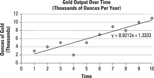
Simple linear regression uses only one feature to predict the target. For example, we use ship age to predict the number of deficiencies of a PSC inspection. Denote the training set with $n$ samples by $D=\left{\left(x_1, y_1\right),\left(x_2, y_2\right), \ldots,\left(x_n, y_n\right)\right}$ and the feature vector by $x$. Simple linear regression aims to develop a model taking the following form:
$$
\hat{y}i=w x_i+b, $$ where $\hat{y}_i$ is the predicted target for sample $i, w$ is the parameter weight and $b$ is the bias. $w$ and $b$ need to be learned from $D$. Then, a natural question is: what are good $w$ and $b$ ? Or in other words, how to find the values of $w$ and $b$ such that the predicted target is as accurate as possible? The key point of developing a simple linear regression model is to evaluate the difference between $\hat{y}_i$ and $y, i=1, \ldots, n$ using the loss function and to adopt the values of $w$ and $b$ that minimize the loss function. In a regression problem, the most commonly used loss function is the mean squared error (MSE), where $M S E=\frac{1}{n} \sum{i=1}^n\left(y_i-\hat{y}_i\right)^2$. Therefore, the learning objective of simple linear regression is to find the optimal $\left(w^, b^\right)$ such that the MSE is minimized. The above idea can be presented by the following mathematical functions:

$$
\begin{aligned}
\left(w^, x^\right) & =\underset{(w, b)}{\arg \min } \sum_{i=1}^n\left(y_i-\hat{y}i\right)^2 \ & =\underset{(w, b)}{\arg \min } \sum{i=1}^n\left(y_i-w x_i-b\right)^2
\end{aligned}
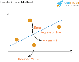
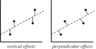
$$
This idea is called the least squares method. The intuition behind it is to minimize the sum of lengths of the vertical lines between all the samples and the regression line determined by $w$ and $b$. It can easily be shown that $M S E$ is convex in $w$ and $b$, and thus $\left(w^, b^\right)$ can be found by
$$
\begin{aligned}
\frac{\partial M S E}{\partial w} & =2\left(\sum_{i=1}^n x_i\left[w x_i-\left(y_i-b\right)\right]\right)=0 \
\Rightarrow w^* & =\frac{\sum_{i=1}^n y_i\left(x_i-\frac{1}{n} \sum_{i=1}^n x_i\right)}{\sum_{i=1}^n x_i^2-\frac{1}{n}\left(\sum_{i=1}^n x_i\right)^2}
\end{aligned}
$$
The optimal $w^$ is first found by Equation (5.2), and then it can be used to calculate the optimal value of $b$, denoted by $b^$, as follows:
$$
\begin{aligned}
& \frac{\partial M S E}{\partial b}=2\left(\sum_{i=1}^n w^* x_i+b-y_i\right)=0 \
& \Rightarrow b^=\frac{1}{n} \sum_{i=1}^n\left(y_i-w^ x_i\right)
\end{aligned}
$$
Simple linear regression can easily be realized by scikit-learn API [1] in Python. Here is ann exannplè of using ship aage to predict ship deficiencyy number using simplé linear regression.

机器学习代考

计算机代写|机器学习代写machine learning代考|The background and development of PSC

PSC由此而生，旨在对各国港口的外国来访船舶进行检查，以验证“船舶及其设备的状况符合国际规则的要求，船舶的配员和操作符合这些规则”。国际海事组织 [7]。在检查过程中，船上出现不符合相关公约要求的情况称为缺陷。船上发现的缺陷的数量和性质决定了 PSC 官员 (PSCO[s]) 采取的相应行动。常见的行动包括在 14 天内或在出发和船舶滞留之前在下一个港口纠正缺陷。尤其，

PSC 检查在区域层面进行。1982年，14个欧洲国家首次签署了关于PSC的谅解备忘录（MoU），称为巴黎谅解备忘录，标志着PSC正式成立。此后，巴黎谅解备忘录的成员国数量不断增加，截至 2022 年 1 月，已有 27 个参与海事管理机构覆盖欧洲沿海国家和北大西洋盆地的海域。另一个大型区域性谅解备忘录在远东地区负责亚太地区，称为东京谅解备忘录，于 1993 年签署。它现在包含 22 个成员国。此外，还有另外七份关于 PSC 的谅解备忘录，即 Acuerdo de Viña del Mar（拉丁美洲）、Caribbean MoU（加勒比）、Abuja MoU（西非和中非）、Black Sea MoU（黑海地区）、Mediterranean米欧在（地中海）、印度洋米欧在（印度洋）和利雅得谅解备忘录。构建谅解备忘录的主要目标是构建完善和统一的PSC体系，加强成员国之间的合作和信息交流，避免在短期内进行多次检查。除了九个区域谅解备忘录外，美国海岸警卫队还维持第十个 PSC 制度。

计算机代写|机器学习代写machine learning代考|Simple linear regression and the least squares

简单线性回归仅使用一个特征来预测目标。例如，我们使用船龄来预测 PSC 检查的缺陷数量。 量 $x$. 简单线性回归旨在开发采用以下形式的模型:
$$
\hat{y} i=w x_i+b,
$$
在哪里 $\hat{y}i$ 是样本的预测目标 $i, w$ 是参数权重和 $b$ 是偏见。 $w$ 和 $b$ 需要借鉴 $D$. 那么，一个自然的问 题是: 什么是好的 $w$ 和 $b$ ? 或者换句话说，如何找到 $w$ 和 $b$ 使得预测的目标尽可能准确? 开发简 单线性回归模型的关键点是评估两者之间的差异 $\hat{y}_i$ 和 $y, i=1, \ldots, n$ 使用损失函数并采用的值 $w$ 和 $b$ 最小化损失函数。在回归问题中，最常用的损失函数是均方误差 (MSE)，其中 $M S E=\frac{1}{n} \sum i=1^n\left(y_i-\hat{y}_i\right)^2$. 因此，简单线性回归的学习目标是找到最优的 $\mid$ beginialigned $} \backslash$ \eft(w^, $x^{\wedge} \backslash$ right) \& $=\backslash$ underset ${(w, b)}{\operatorname{larg} \backslash \min } \backslash$ Isum{i $\left._1\right}^{\wedge} \backslash \backslash e f t\left(y _i-\backslash h a t{y} i \backslash r i g h t\right)^{\wedge} 2 \backslash$
这个想法被称为最小二乘法。其背后的直觉是最小化所有样本之间的垂直线的长度总和以及由
$$
\frac{\partial M S E}{\partial w}=2\left(\sum_{i=1}^n x_i\left[w x_i-\left(y_i-b\right)\right]\right)=0 \Rightarrow w^* \quad=\frac{\sum_{i=1}^n y_i\left(x_i-\frac{1}{n} \sum_{i=1}^n x_i\right)}{\sum_{i=1}^n x_i^2-\frac{1}{n}\left(\sum_{i=1}^n x_i\right)^2}
$$
最优的^先由式 (5.2) 求得，然后可用于计算最优值 $b$, 表示为 $\mathrm{b}^{\wedge}$ ，如下:
$$
\frac{\partial M S E}{\partial b}=2\left(\sum_{i=1}^n w^* x_i+b-y_i\right)=0 \quad \Rightarrow b^{=} \frac{1}{n} \sum_{i=1}^n\left(y_i-w_i^x\right)
$$
Python 中的 scikit-learn API [1] 可以轻松实现简单的线性回归。这是使用船舶年龄通过简单线 性回归预测船舶缺陷数量的示例。

统计代写请认准statistics-lab™. statistics-lab™为您的留学生涯保驾护航。

金融工程代写

金融工程是使用数学技术来解决金融问题。金融工程使用计算机科学、统计学、经济学和应用数学领域的工具和知识来解决当前的金融问题，以及设计新的和创新的金融产品。

非参数统计代写

非参数统计指的是一种统计方法，其中不假设数据来自于由少数参数决定的规定模型；这种模型的例子包括正态分布模型和线性回归模型。

广义线性模型代考

广义线性模型（GLM）归属统计学领域，是一种应用灵活的线性回归模型。该模型允许因变量的偏差分布有除了正态分布之外的其它分布。

术语 广义线性模型（GLM）通常是指给定连续和/或分类预测因素的连续响应变量的常规线性回归模型。它包括多元线性回归，以及方差分析和方差分析（仅含固定效应）。

有限元方法代写

有限元方法（FEM）是一种流行的方法，用于数值解决工程和数学建模中出现的微分方程。典型的问题领域包括结构分析、传热、流体流动、质量运输和电磁势等传统领域。

有限元是一种通用的数值方法，用于解决两个或三个空间变量的偏微分方程（即一些边界值问题）。为了解决一个问题，有限元将一个大系统细分为更小、更简单的部分，称为有限元。这是通过在空间维度上的特定空间离散化来实现的，它是通过构建对象的网格来实现的：用于求解的数值域，它有有限数量的点。边界值问题的有限元方法表述最终导致一个代数方程组。该方法在域上对未知函数进行逼近。[1] 然后将模拟这些有限元的简单方程组合成一个更大的方程系统，以模拟整个问题。然后，有限元通过变化微积分使相关的误差函数最小化来逼近一个解决方案。

tatistics-lab作为专业的留学生服务机构，多年来已为美国、英国、加拿大、澳洲等留学热门地的学生提供专业的学术服务，包括但不限于Essay代写，Assignment代写，Dissertation代写，Report代写，小组作业代写，Proposal代写，Paper代写，Presentation代写，计算机作业代写，论文修改和润色，网课代做，exam代考等等。写作范围涵盖高中，本科，研究生等海外留学全阶段，辐射金融，经济学，会计学，审计学，管理学等全球99%专业科目。写作团队既有专业英语母语作者，也有海外名校硕博留学生，每位写作老师都拥有过硬的语言能力，专业的学科背景和学术写作经验。我们承诺100%原创，100%专业，100%准时，100%满意。

随机分析代写

随机微积分是数学的一个分支，对随机过程进行操作。它允许为随机过程的积分定义一个关于随机过程的一致的积分理论。这个领域是由日本数学家伊藤清在第二次世界大战期间创建并开始的。

时间序列分析代写

随机过程，是依赖于参数的一组随机变量的全体，参数通常是时间。 随机变量是随机现象的数量表现，其时间序列是一组按照时间发生先后顺序进行排列的数据点序列。通常一组时间序列的时间间隔为一恒定值（如1秒，5分钟，12小时，7天，1年），因此时间序列可以作为离散时间数据进行分析处理。研究时间序列数据的意义在于现实中，往往需要研究某个事物其随时间发展变化的规律。这就需要通过研究该事物过去发展的历史记录，以得到其自身发展的规律。

回归分析代写

多元回归分析渐进（Multiple Regression Analysis Asymptotics）属于计量经济学领域，主要是一种数学上的统计分析方法，可以分析复杂情况下各影响因素的数学关系，在自然科学、社会和经济学等多个领域内应用广泛。

MATLAB代写

MATLAB 是一种用于技术计算的高性能语言。它将计算、可视化和编程集成在一个易于使用的环境中，其中问题和解决方案以熟悉的数学符号表示。典型用途包括：数学和计算算法开发建模、仿真和原型制作数据分析、探索和可视化科学和工程图形应用程序开发，包括图形用户界面构建MATLAB 是一个交互式系统，其基本数据元素是一个不需要维度的数组。这使您可以解决许多技术计算问题，尤其是那些具有矩阵和向量公式的问题，而只需用 C 或 Fortran 等标量非交互式语言编写程序所需的时间的一小部分。MATLAB 名称代表矩阵实验室。MATLAB 最初的编写目的是提供对由 LINPACK 和 EISPACK 项目开发的矩阵软件的轻松访问，这两个项目共同代表了矩阵计算软件的最新技术。MATLAB 经过多年的发展，得到了许多用户的投入。在大学环境中，它是数学、工程和科学入门和高级课程的标准教学工具。在工业领域，MATLAB 是高效研究、开发和分析的首选工具。MATLAB 具有一系列称为工具箱的特定于应用程序的解决方案。对于大多数 MATLAB 用户来说非常重要，工具箱允许您学习和应用专业技术。工具箱是 MATLAB 函数（M 文件）的综合集合，可扩展 MATLAB 环境以解决特定类别的问题。可用工具箱的领域包括信号处理、控制系统、神经网络、模糊逻辑、小波、仿真等。

R语言代写	问卷设计与分析代写
PYTHON代写	回归分析与线性模型代写
MATLAB代写	方差分析与试验设计代写
STATA代写	机器学习/统计学习代写
SPSS代写	计量经济学代写
EVIEWS代写	时间序列分析代写
EXCEL代写	深度学习代写
SQL代写	各种数据建模与可视化代写

如果你也在 怎样代写机器学习 machine learning这个学科遇到相关的难题，请随时右上角联系我们的24/7代写客服。

机器学习是一个致力于理解和建立 “学习 “方法的研究领域，也就是说，利用数据来提高某些任务的性能的方法。机器学习算法基于样本数据（称为训练数据）建立模型，以便在没有明确编程的情况下做出预测或决定。机器学习算法被广泛用于各种应用，如医学、电子邮件过滤、语音识别和计算机视觉，在这些应用中，开发传统算法来执行所需任务是困难的或不可行的。

statistics-lab™ 为您的留学生涯保驾护航 在代写机器学习 machine learning方面已经树立了自己的口碑, 保证靠谱, 高质且原创的统计Statistics代写服务。我们的专家在代写机器学习 machine learning代写方面经验极为丰富，各种代写机器学习 machine learning相关的作业也就用不着说。

我们提供的机器学习 machine learning及其相关学科的代写，服务范围广, 其中包括但不限于:

• Statistical Inference 统计推断
• Statistical Computing 统计计算
• Advanced Probability Theory 高等概率论
• Advanced Mathematical Statistics 高等数理统计学
• (Generalized) Linear Models 广义线性模型
• Statistical Machine Learning 统计机器学习
• Longitudinal Data Analysis 纵向数据分析
• Foundations of Data Science 数据科学基础

计算机代写|机器学习代写machine learning代考|Container liner shipping

A majority of cargoes in supermarkets, such as fruits and vegetables, kitchen appliances, furniture, garments, meats, fish, dairy products, and toys, are transported in containers by ship. Containers are usually expressed in terms of TEUs, a box that is 20 feet long $(6.1 \mathrm{~m})$. Throughout this book, unless otherwise specified, we use “TEU” to express “the number of containers” or “the volume of containers.”

Containers are transported by ship on liner services, which are similar to bus services. Figure $1.1$ is the Central China $2(\mathrm{CC} 2)$ service operated by Orient Overseas Container Line (OOCL), a Hong Kong-based shipping company. We call it a service, a route, or a service route. A route is a loop, and the port rotation of a route is the sequence of ports of call on the route. Any port of call can be defined as the first port of call. For example, if we define Ningbo as the first port of call, then Shanghai is the second port of call, and Los Angeles is the third port of call. We can therefore represent the port rotation of the route as follows:
Ningbo (1) $\rightarrow$ Shanghai $(2) \rightarrow$ Los Angeles $(3) \rightarrow$ Ningbo (1)

Note that on a route, different ports of call may be the same physical port. For example, the Central China 1 (CC1) service of OOCL shown in Figure $1.2$ has the port rotation below:

Shanghai (1) $\rightarrow$ Kwangyang (2) $\rightarrow$ Pusan (3) $\rightarrow$ Los Angeles (4) $\rightarrow$ Oakland $(5) \rightarrow$ Pusan $(6) \rightarrow$ Kwangyang $(7) \rightarrow$ Shanghai (1)

Both the second and the seventh ports of call are Kwangyang, and both the third and the sixth ports of call are Pusan.

A leg is the voyage from one port of call to the next. Leg $i$ is the voyage from the $i$ th port of call to port of call $i+1$. The last leg is the voyage from the last port of call to the first port of call. On CCl, the second leg is the voyage from Kwangyang (the second) to Pusan (the third), and the seventh leg is the voyage from Kwangyang (the seventh) to Shanghai (the first).

The rotation time of a route is the time required for a ship to start from the first port of call, visit all ports of call on the route, and return to the first port of call. As can be read from Figures $1.1$ and 1.2, the rotation time of $\mathrm{CC} 2$ is 35 days*, and the rotation time of $\mathrm{CC} 1$ is 42 days. Each route provides a weekly frequency, which means that each port of call is visited on the same day every week. Therefore, a string of five ships are deployed on $\mathrm{CC} 2$, and the headway between two adjacent ships is 7 days. These five ships usually have the same TEU capacity and other characteristics. Unless otherwise specified, we assume weekly frequencies for all routes.

计算机代写|机器学习代写machine learning代考|Key issues in maritime transport

Maritime transport is a highly globalized industry in terms of operation and management. For ship operation, ocean-going vessels sail on the high seas from the origin port in one country/region to the destination port in another country/region. For ship management, parties responsible for ship ownership, crewing, and operating may locate in different countries and regions. Even the country of registration, i.e., ship flag state, may not have a direct link and connection with a ship’s activities as the ship may not frequently visit the ports belonging to its flag state. For inland countries such as Mongolia, the ships registered under it never visit its ports. Such complex and disintegrated nature of the shipping industry makes it hard to control and regulate international shipping activities, and thus pose danger to maritime safety, the marine environment, and the crew and cargoes carried by ocean-going vessels.
Shipping is one of the world’s most dangerous industries due to the complex and ever-changing environment at sea, the dangerous goods carried, and the difficulties in search and rescue. Safety at sea is always put at the highest priority in ship operation and management. It is widely believed that the most effective and efficient way of improving safety at sea is to develop international regulations that should be followed by all shipping nations [1]. A unified and permanent international body was expected to be established for regulation and supervision by several nations from the mid-19th century onward, and the hopes came true after the International Maritime Organization (IMO, whose original name was Inter-Governmental Maritime Consultative Organization) was established at an international conference in Geneva held in 1948. Through hard efforts of all parties, the members of IMO met for the first time in 1959, one year after the IMO convention came into force. The IMO’s task was to adopt a new version of the most important conventions on maritime safety, i.e., the International Convention for the Safety of Life at Sea, which specifies minimum safety standards for ship construction, equipment, and operation. It covers comprehensive aspects of shipping safety, including vessel construction, fire safety, life-saving arrangements, radio communications, navigation safety, cargo carriage, dangerous goods transporting, the mandatory of the International Safety Management (ISM) code, verification of compliance, and measures for specific ships, and is constantly amended [2]. The Maritime Safety Committee is responsible for every aspect of maritime safety and security, and it is the highest technical body of the IMO.

机器学习代考

计算机代写|机器学习代写machine learning代考|Container liner shipping

超市的大部分货物，如水果和蔬菜、厨房用具、家具、服装、肉类、鱼类、乳制品和玩具，都 是通过集装箱通过船舶运输的。集装箱通常以 TEU 表示，一个20 英尺长的箱子 $(6.1 \mathrm{~m})$. 在本 书中，除非另有说明，否则我们使用“TEU”来表示“集装箱数量”或”集装箱体积”。
集装箱由班轮服务的船舶运输，类似于巴士服务。数字 $1.1$ 是中原 $2(\mathrm{CC} 2)$ 服务由总部位于香 港的航运公司东方海外货柜航运公司 (OOCL) 运营。我们称之为服务、路线或服务路线。路由 是一个循环，路由的端口轮换是路由上的调用端口的顺序。任何停靠港都可以定义为第一停靠 港。例如，如果我们将宁波定义为第一停靠港，那么上海就是第二停靠港，洛杉矶就是第三停 靠港。因此，我们可以表示航线的港口轮换如下:
宁波 (1) $\rightarrow$ Shanghai (2) $\rightarrow$ 天使(3) $\rightarrow$ Ningbo (1)
请注意，在一条路刬上，不同的呼叫端口可能是相同的物理端口。例如东方海外的华中一号 (CC1）服务如图 $1.2$ 具有以下端口旋转:

Shanghai (1) →光阳 (2)→滏山 (3)→洛杉矶 (4)→奥克兰 $(5) \rightarrow$ 釜山(6) →光阳(7) $\rightarrow$ Shanghai (1)
第二和第七停靠港都是光阳，第三和第六停靠港都是釜山。
航程是从一个停靠港到下一个停靠港的航程。腿航程是从 $i$ th 停靠港到停靠港 $i+1$. 最后一航 程是从最后一个停靠港到第一个停靠港的航程。CCL上，第二航程为光阳 (第二) 至釜山 (第 三) 航次，第七航程为光阳 (第七) 至上海 (第一) 航次。
航线轮转时间是指船舶从第一个停靠港出发，经过航线上所有停靠港，返回到第一个停靠港所 需的时间。从图中可以看出 $1.1$ 和 1.2，旋转时间 $\mathrm{CC} 2$ 为 $35 天^*$ ，轮换时间为 $\mathrm{CC} 1$ 是 42 天。每 条航线隄供每周频率，这意味着每个停靠港在每周的同一天到达。因此，一连串的五艘船部署 在CC2, 相邻两船之间的船头间隔为 7 天。这五艘船通常具有相同的 TEU容量和其他特征。除 非另有说明，否则我们假定所有路线每周一班。

计算机代写|机器学习代写machine learning代考|Key issues in maritime transport

海运业是一个经营管理高度全球化的行业。对于船舶作业，远洋船舶从一个国家/地区的始发港到另一国家/地区的目的港在公海航行。对于船舶管理，负责船舶所有权、船员和运营的各方可能位于不同的国家和地区。即使是注册国，即船旗国，也可能与船舶的活动没有直接联系，因为船舶可能不会经常访问属于其船旗国的港口。对于蒙古等内陆国家，注册在其名下的船舶从不到访其港口。航运业如此复杂和分散的性质使其难以控制和规范国际航运活动，从而对海上安全构成威胁，
由于海上环境复杂多变、载运危险品多、搜救难度大，航运业是世界上最危险的行业之一。海上安全始终是船舶运营管理的重中之重。人们普遍认为，提高海上安全的最有效和高效的方法是制定所有航运国家都应遵守的国际法规 [1]。从19世纪中叶开始，几个国家就期望建立一个统一的永久性国际机构来进行监管和监督，而在国际海事组织（IMO，原名政府间海事协商组织）之后，希望得以实现1948 年在日内瓦举行的一次国际会议上成立。经过各方的努力，IMO成员于1959年举行首次会议，即IMO公约生效一年后。IMO 的任务是采用最重要的海事安全公约的新版本，即国际海上人命安全公约，其中规定了船舶建造、设备和操作的最低安全标准。它涵盖了航运安全的各个方面，包括船舶建造、消防安全、救生安排、无线电通信、航行安全、货物运输、危险品运输、国际安全管理 (ISM) 规则的强制性、合规性验证以及针对特定船舶的措施，并不断修订[2]。海上安全委员会负责海上安全和安保的各个方面，

统计代写请认准statistics-lab™. statistics-lab™为您的留学生涯保驾护航。

金融工程代写

金融工程是使用数学技术来解决金融问题。金融工程使用计算机科学、统计学、经济学和应用数学领域的工具和知识来解决当前的金融问题，以及设计新的和创新的金融产品。

非参数统计代写

非参数统计指的是一种统计方法，其中不假设数据来自于由少数参数决定的规定模型；这种模型的例子包括正态分布模型和线性回归模型。

广义线性模型代考

广义线性模型（GLM）归属统计学领域，是一种应用灵活的线性回归模型。该模型允许因变量的偏差分布有除了正态分布之外的其它分布。

术语 广义线性模型（GLM）通常是指给定连续和/或分类预测因素的连续响应变量的常规线性回归模型。它包括多元线性回归，以及方差分析和方差分析（仅含固定效应）。

有限元方法代写

有限元方法（FEM）是一种流行的方法，用于数值解决工程和数学建模中出现的微分方程。典型的问题领域包括结构分析、传热、流体流动、质量运输和电磁势等传统领域。

有限元是一种通用的数值方法，用于解决两个或三个空间变量的偏微分方程（即一些边界值问题）。为了解决一个问题，有限元将一个大系统细分为更小、更简单的部分，称为有限元。这是通过在空间维度上的特定空间离散化来实现的，它是通过构建对象的网格来实现的：用于求解的数值域，它有有限数量的点。边界值问题的有限元方法表述最终导致一个代数方程组。该方法在域上对未知函数进行逼近。[1] 然后将模拟这些有限元的简单方程组合成一个更大的方程系统，以模拟整个问题。然后，有限元通过变化微积分使相关的误差函数最小化来逼近一个解决方案。

tatistics-lab作为专业的留学生服务机构，多年来已为美国、英国、加拿大、澳洲等留学热门地的学生提供专业的学术服务，包括但不限于Essay代写，Assignment代写，Dissertation代写，Report代写，小组作业代写，Proposal代写，Paper代写，Presentation代写，计算机作业代写，论文修改和润色，网课代做，exam代考等等。写作范围涵盖高中，本科，研究生等海外留学全阶段，辐射金融，经济学，会计学，审计学，管理学等全球99%专业科目。写作团队既有专业英语母语作者，也有海外名校硕博留学生，每位写作老师都拥有过硬的语言能力，专业的学科背景和学术写作经验。我们承诺100%原创，100%专业，100%准时，100%满意。

随机分析代写

随机微积分是数学的一个分支，对随机过程进行操作。它允许为随机过程的积分定义一个关于随机过程的一致的积分理论。这个领域是由日本数学家伊藤清在第二次世界大战期间创建并开始的。

时间序列分析代写

随机过程，是依赖于参数的一组随机变量的全体，参数通常是时间。 随机变量是随机现象的数量表现，其时间序列是一组按照时间发生先后顺序进行排列的数据点序列。通常一组时间序列的时间间隔为一恒定值（如1秒，5分钟，12小时，7天，1年），因此时间序列可以作为离散时间数据进行分析处理。研究时间序列数据的意义在于现实中，往往需要研究某个事物其随时间发展变化的规律。这就需要通过研究该事物过去发展的历史记录，以得到其自身发展的规律。

回归分析代写

多元回归分析渐进（Multiple Regression Analysis Asymptotics）属于计量经济学领域，主要是一种数学上的统计分析方法，可以分析复杂情况下各影响因素的数学关系，在自然科学、社会和经济学等多个领域内应用广泛。

MATLAB代写

MATLAB 是一种用于技术计算的高性能语言。它将计算、可视化和编程集成在一个易于使用的环境中，其中问题和解决方案以熟悉的数学符号表示。典型用途包括：数学和计算算法开发建模、仿真和原型制作数据分析、探索和可视化科学和工程图形应用程序开发，包括图形用户界面构建MATLAB 是一个交互式系统，其基本数据元素是一个不需要维度的数组。这使您可以解决许多技术计算问题，尤其是那些具有矩阵和向量公式的问题，而只需用 C 或 Fortran 等标量非交互式语言编写程序所需的时间的一小部分。MATLAB 名称代表矩阵实验室。MATLAB 最初的编写目的是提供对由 LINPACK 和 EISPACK 项目开发的矩阵软件的轻松访问，这两个项目共同代表了矩阵计算软件的最新技术。MATLAB 经过多年的发展，得到了许多用户的投入。在大学环境中，它是数学、工程和科学入门和高级课程的标准教学工具。在工业领域，MATLAB 是高效研究、开发和分析的首选工具。MATLAB 具有一系列称为工具箱的特定于应用程序的解决方案。对于大多数 MATLAB 用户来说非常重要，工具箱允许您学习和应用专业技术。工具箱是 MATLAB 函数（M 文件）的综合集合，可扩展 MATLAB 环境以解决特定类别的问题。可用工具箱的领域包括信号处理、控制系统、神经网络、模糊逻辑、小波、仿真等。

R语言代写	问卷设计与分析代写
PYTHON代写	回归分析与线性模型代写
MATLAB代写	方差分析与试验设计代写
STATA代写	机器学习/统计学习代写
SPSS代写	计量经济学代写
EVIEWS代写	时间序列分析代写
EXCEL代写	深度学习代写
SQL代写	各种数据建模与可视化代写

如果你也在 怎样代写机器学习 machine learning这个学科遇到相关的难题，请随时右上角联系我们的24/7代写客服。

机器学习是一个致力于理解和建立 “学习 “方法的研究领域，也就是说，利用数据来提高某些任务的性能的方法。机器学习算法基于样本数据（称为训练数据）建立模型，以便在没有明确编程的情况下做出预测或决定。机器学习算法被广泛用于各种应用，如医学、电子邮件过滤、语音识别和计算机视觉，在这些应用中，开发传统算法来执行所需任务是困难的或不可行的。

statistics-lab™ 为您的留学生涯保驾护航 在代写机器学习 machine learning方面已经树立了自己的口碑, 保证靠谱, 高质且原创的统计Statistics代写服务。我们的专家在代写机器学习 machine learning代写方面经验极为丰富，各种代写机器学习 machine learning相关的作业也就用不着说。

我们提供的机器学习 machine learning及其相关学科的代写，服务范围广, 其中包括但不限于:

• Statistical Inference 统计推断
• Statistical Computing 统计计算
• Advanced Probability Theory 高等概率论
• Advanced Mathematical Statistics 高等数理统计学
• (Generalized) Linear Models 广义线性模型
• Statistical Machine Learning 统计机器学习
• Longitudinal Data Analysis 纵向数据分析
• Foundations of Data Science 数据科学基础

计算机代写|机器学习代写machine learning代考|Intuition and Main Results

Consider first the training error $E_{\text {train }}$ defined in (5.3). Since
$$
\operatorname{tr} \mathbf{Y} \mathbf{Q}^2(\gamma) \mathbf{Y}^{\boldsymbol{\top}}=-\frac{\partial}{\partial \gamma} \operatorname{tr} \mathbf{Y} \mathbf{Q}(\gamma) \mathbf{Y}^{\top},
$$
a deterministic equivalent for the resolvent $\mathbf{Q}(\gamma)$ is sufficient to acceess the asymptotic behavior of $E_{\text {train }}$.
With a linear activation $\sigma(t)=t$, the resolvent of interest
$$
\mathbf{Q}(\gamma)=\left(\frac{1}{n} \sigma(\mathbf{W X})^{\top} \sigma(\mathbf{W} \mathbf{X})+\gamma \mathbf{I}n\right)^{-1} $$ is the same as in Theorem 2.6. In a sense, the evaluation of $\mathbf{Q}(\gamma)$ (and subsequently $\left.E{\text {train }}\right)$ calls for an extension of Theorem $2.6$ to handle the case of nonlinear activations. Recall now that the main ingredients to derive a deterministic equivalent for (the linear case) $\mathbf{Q}=\left(\mathbf{X}^{\top} \mathbf{W}^{\top} \mathbf{W} \mathbf{X} / n+\gamma \mathbf{I}n\right)^{-1}$ are (i) $\mathbf{X}^{\top} \mathbf{W}^{\top}$ has i.i.d. columns and (ii) its $i$ th column $\left[\mathbf{W}^{\top}\right]_i$ has i.i.d. (or linearly dependent) entries so that the key Lemma $2.11$ applies. These hold, in the linear case, due to the i.i.d. property of the entries of $\mathbf{W}$. However, while for Item (i), the nonlinear $\Sigma^{\top}=\sigma(\mathbf{W X})^{\top}$ still has i.i.d. columns, and for Item (ii), its $i$ th column $\sigma\left(\left[\mathbf{X}^{\top} \mathbf{W}^{\top}\right]{. i}\right)$ no longer has i.i.d. or linearly dependent entries. Therefore, the main technical difficulty here is to obtain a nonlinear version of the trace lemma, Lemma 2.11. That is, we expect that the concentration of quadratic forms around their expectation remains valid despite the application of the entry-wise nonlinear $\sigma$. This naturally falls into the concentration of measure theory discussed in Section $2.7$ and is given by the following lemma.

Lemma 5.1 (Concentration of nonlinear quadratic form, Louart et al. [2018, Lemma 1]). For $\mathbf{w} \sim \mathcal{N}\left(\mathbf{0}, \mathbf{I}_p\right)$, 1-Lipschitz $\sigma(\cdot)$, and $\mathbf{A} \in \mathbb{R}^{n \times n}, \mathbf{X} \in \mathbb{R}^{p \times n}$ such that $|\mathbf{A}| \leq 1$ and $|\mathbf{X}|$ bounded with respect to $p, n$, then,
$$
\mathbb{P}\left(\left|\frac{1}{n} \sigma\left(\mathbf{w}^{\top} \mathbf{X}\right) \mathbf{A} \sigma\left(\mathbf{X}^{\top} \mathbf{w}\right)-\frac{1}{n} \operatorname{tr} \mathbf{A} \mathbf{K}\right|>t\right) \leq C e^{-c n \min \left(t, t^2\right)}
$$ for some $C, c>0, p / n \in(0, \infty)$ with ${ }^2$
$$
\mathbf{K} \equiv \mathbf{K}{\mathbf{X X}} \equiv \mathbb{E}{\mathbf{w} \sim \mathcal{N}\left(\mathbf{0}, \mathbf{I}_p\right)}\left[\sigma\left(\mathbf{X}^{\top} \mathbf{w}\right) \sigma\left(\mathbf{w}^{\boldsymbol{\top}} \mathbf{X}\right)\right] \in \mathbb{R}^{n \times n}
$$

计算机代写|机器学习代写machine learning代考|Consequences for Learning with Large Neural Networks

To validate the asymptotic analysis in Theorem $5.1$ and Corollary $5.1$ on real-world data, Figures $5.2$ and $5.3$ compare the empirical MSEs with their limiting behavior predicted in Corollary 5.1, for a random network of $N=512$ neurons and various types of Lipschitz and non-Lipschitz activations $\sigma(\cdot)$, respectively. The regressor $\boldsymbol{\beta} \in \mathbb{R}^p$ maps the vectorized images from the Fashion-MNIST dataset (classes 1 and 2) [Xiao et al., 2017] to their corresponding uni-dimensional ( $d=1$ ) output labels $\mathbf{Y}{1 i}, \hat{\mathbf{Y}}{1 j} \in$ ${\pm 1}$. For $n, p, N$ of order a few hundreds (so not very large when compared to typical modern neural network dimensions), a close match between theory and practice is observed for the Lipschitz activations in Figure 5.2. The precision is less accurate but still quite good for the case of non-Lipschitz activations in Figure 5.3, which, we recall, are formally not supported by the theorem statement – here for $\sigma(t)=1-t^2 / 2$, $\sigma(t)=1_{t>0}$, and $\sigma(t)=\operatorname{sign}(t)$. For all activations, the deviation from theory is more acute for small values of regularization $\gamma$.

Figures $5.2$ and $5.3$ confirm that while the training error is a monotonically increasing function of the regularization parameter $\gamma$, there always exists an optimal value for $\gamma$ which minimizes the test error. In particular, the theoretical formulas derived in Corollary $5.1$ allow for a (data-dependent) fast offline tuning of the hyperparameter $\gamma$ of the network, in the setting where $n, p, N$ are not too small and comparable. In terms of activation functions (those listed here), we observe that, on the Fashion-MNIST dataset, the ReLU nonlinearity $\sigma(t)=\max (t, 0)$ is optimal and achieves the minimum test error, while the quadratic activation $\sigma(t)=1-t^2 / 2$ is the worst and produces much higher training and test errors compared to others. This observation will be theoretically explained through a deeper analysis of the corresponding kernel matrix $\mathbf{K}$, as performed in Section 5.1.2. Lastly, although not immediate at first sight, the training and test error curves of $\sigma(t)=1_{t>0}$ and $\sigma(t)=\operatorname{sign}(t)$ are indeed the same, up to a shift in $\gamma$, as a consequence of the fact that $\operatorname{sign}(t)=2 \cdot 1_{t>0}-1$.

机器学习代考

计算机代写|机器学习代写machine learning代考|Intuition and Main Results

首先考虑训练误差 $E_{\text {train }}$ 在 (5.3) 中定义。自从
$$
\operatorname{tr} \mathbf{Y} \mathbf{Q}^2(\gamma) \mathbf{Y}^{\top}=-\frac{\partial}{\partial \gamma} \operatorname{tr} \mathbf{Y} \mathbf{Q}(\gamma) \mathbf{Y}^{\top}
$$
解决方案的确定性等价物 $\mathbf{Q}(\gamma)$ 足以访问的渐近行为 $E_{\text {train }}$.
线性激活 $\sigma(t)=t$ ，感兴趣的溶剂
$$
\mathbf{Q}(\gamma)=\left(\frac{1}{n} \sigma(\mathbf{W X})^{\top} \sigma(\mathbf{W X})+\gamma \mathbf{I} n\right)^{-1}
$$
与定理 $2.6$ 相同。从某种意义上说，评价 $\mathbf{Q}(\gamma)$ (随后 $E \operatorname{train}$ )要求扩展定理 $2.6$ 处理非线性激活的情 况。现在回想一下，推导出 (线性情况) 的确定性等价物的主要成分
$\mathbf{Q}=\left(\mathbf{X}^{\top} \mathbf{W}^{\top} \mathbf{W X} / n+\gamma \mathbf{I} n\right)^{-1}$ 是我) $\mathbf{X}^{\top} \mathbf{W}^{\top}$ 有 iid 列和 (ii) 它的 $i$ 第 列 $\left[\mathbf{W}^{\top}\right]_i$ 具有独立同分布 (或线性相关) 条目，因此密钥引理 $2.11$ 适用。在线性情况下，由于条目的 iid 属性，这些成立 W. 然 而，对于项目 (i)，非线性 $\Sigma^{\top}=\sigma(\mathbf{W X})^{\top}$ 仍然有 iid 列，对于项目 (ii)，其 $i$ 第列 $\sigma\left(\left[\mathbf{X}^{\top} \mathbf{W}^{\top}\right] . i\right)$ 不 再具有 iid 或线性相关条目。因此，这里的主要技术难点是获得非线性版本的迹引理，引理 2.11。也就是 说，我们预计尽管应用了逐项非线性 $\sigma$. 这自然落入第 节讨论的测度论的集中 $2.7$ 并由以下引理给出。
引理 $5.1$ (非线性二次型的集中，Louart 等人 [2018，引理 1])。为了 $\mathbf{w} \sim \mathcal{N}\left(\mathbf{0}, \mathbf{I}_p\right)$, 1-利普㹷茨 $\sigma(\cdot)$ ，和 $\mathbf{A} \in \mathbb{R}^{n \times n}, \mathbf{X} \in \mathbb{R}^{p \times n}$ 这样 $|\mathbf{A}| \leq 1$ 和 $|\mathbf{X}|$ 有界于 $p, n$ ，然后，
$$
\mathbb{P}\left(\left|\frac{1}{n} \sigma\left(\mathbf{w}^{\top} \mathbf{X}\right) \mathbf{A} \sigma\left(\mathbf{X}^{\top} \mathbf{w}\right)-\frac{1}{n} \operatorname{tr} \mathbf{A K}\right|>t\right) \leq C e^{-c n \min \left(t, t^2\right)}
$$
对于一些 $C, c>0, p / n \in(0, \infty)$ 和 $^2$
$$
\mathbf{K} \equiv \mathbf{K X X} \equiv \mathbb{E} \mathbf{w} \sim \mathcal{N}\left(\mathbf{0}, \mathbf{I}_p\right)\left[\sigma\left(\mathbf{X}^{\top} \mathbf{w}\right) \sigma\left(\mathbf{w}^{\top} \mathbf{X}\right)\right] \in \mathbb{R}^{n \times n}
$$

计算机代写|机器学习代写machine learning代考|Consequences for Learning with Large Neural Networks

验证定理中的渐近分析5.1和推论 $5.1$ 关于真实世界的数据，数字 $5.2$ 和 $5.3$ 对于一个随机网络，将经验 MSE 与推论 $5.1$ 中预测的限制行为进行比较 $N=512$ 神经元和各种类型的 Lipschitz 和非 Lipschitz 激活 $\sigma(\cdot)$ ，分别。回归者 $\beta \in \mathbb{R}^p$ 将来自 Fashion-MNIST 数据集（第 1 类和第 2 类） [Xiao et al.，2017] 的矢 量化图像映射到它们相应的单维 $(d=1$ ) 输出标签 $\mathbf{Y} 1 i, \hat{\mathbf{Y}} 1 j \in \pm 1$. 为了 $n, p, N$ 数百个数量级 (因此 与典型的现代神经网络维度相比不是很大)，在图 $5.2$ 中观察到 Lipschitz 激活的理论与实践之间的紧密 匹配。精度不太准确，但对于图 $5.3$ 中非 Lipschitz 激活的情况仍然相当不错，我们记得，定理陈述正式 不支持这种情况一一这里是为了 $\sigma(t)=1-t^2 / 2 ， \sigma(t)=1_{t>0}$ ，和 $\sigma(t)=\operatorname{sign}(t)$. 对于所有激活， 正则化的小值与理论的偏差更为严重 $\gamma$.
数字 $5.2$ 和 $5.3$ 确认虽然训练误差是正则化参数的单调递增函数 $\gamma$ ，总是存在一个最优值 $\gamma$ 从而最小化测试误 差。特别是推论中推导出的理论公式5.1允许对超参数进行 (依赖于数据的) 快速离线调整 $\gamma$ 网络的设置 $n, p, N$ 不是太小且具有可比性。就激活函数（此处列出的那些) 而言，我们观察到，在 Fashion-MNIST 数据集上， $\operatorname{ReLU}$ 非线性 $\sigma(t)=\max (t, 0)$ 是最优的并达到最小测试误差，而二次激活 $\sigma(t)=1-t^2 / 2$ 是最差的，与其他人相比会产生更高的训练和测试错误。将通过对相应核矩阵的更深 入分析从理论上解释这一观察结果 $\mathbf{K}$ ，如第 5.1.2 节中所述。最后，虽然乍一看不是立即的，但训练和测试误差曲线 $\sigma(t)=1_{t>0}$ 和 $\sigma(t)=\operatorname{sign}(t)$ 确实是一样的，直到一个转变 $\gamma$ ，由于这样的事实 $\operatorname{sign}(t)=2 \cdot 1_{t>0}-1$

统计代写请认准statistics-lab™. statistics-lab™为您的留学生涯保驾护航。

金融工程代写

金融工程是使用数学技术来解决金融问题。金融工程使用计算机科学、统计学、经济学和应用数学领域的工具和知识来解决当前的金融问题，以及设计新的和创新的金融产品。

非参数统计代写

非参数统计指的是一种统计方法，其中不假设数据来自于由少数参数决定的规定模型；这种模型的例子包括正态分布模型和线性回归模型。

广义线性模型代考

广义线性模型（GLM）归属统计学领域，是一种应用灵活的线性回归模型。该模型允许因变量的偏差分布有除了正态分布之外的其它分布。

术语 广义线性模型（GLM）通常是指给定连续和/或分类预测因素的连续响应变量的常规线性回归模型。它包括多元线性回归，以及方差分析和方差分析（仅含固定效应）。

有限元方法代写

有限元方法（FEM）是一种流行的方法，用于数值解决工程和数学建模中出现的微分方程。典型的问题领域包括结构分析、传热、流体流动、质量运输和电磁势等传统领域。

有限元是一种通用的数值方法，用于解决两个或三个空间变量的偏微分方程（即一些边界值问题）。为了解决一个问题，有限元将一个大系统细分为更小、更简单的部分，称为有限元。这是通过在空间维度上的特定空间离散化来实现的，它是通过构建对象的网格来实现的：用于求解的数值域，它有有限数量的点。边界值问题的有限元方法表述最终导致一个代数方程组。该方法在域上对未知函数进行逼近。[1] 然后将模拟这些有限元的简单方程组合成一个更大的方程系统，以模拟整个问题。然后，有限元通过变化微积分使相关的误差函数最小化来逼近一个解决方案。

tatistics-lab作为专业的留学生服务机构，多年来已为美国、英国、加拿大、澳洲等留学热门地的学生提供专业的学术服务，包括但不限于Essay代写，Assignment代写，Dissertation代写，Report代写，小组作业代写，Proposal代写，Paper代写，Presentation代写，计算机作业代写，论文修改和润色，网课代做，exam代考等等。写作范围涵盖高中，本科，研究生等海外留学全阶段，辐射金融，经济学，会计学，审计学，管理学等全球99%专业科目。写作团队既有专业英语母语作者，也有海外名校硕博留学生，每位写作老师都拥有过硬的语言能力，专业的学科背景和学术写作经验。我们承诺100%原创，100%专业，100%准时，100%满意。

随机分析代写

随机微积分是数学的一个分支，对随机过程进行操作。它允许为随机过程的积分定义一个关于随机过程的一致的积分理论。这个领域是由日本数学家伊藤清在第二次世界大战期间创建并开始的。

时间序列分析代写

随机过程，是依赖于参数的一组随机变量的全体，参数通常是时间。 随机变量是随机现象的数量表现，其时间序列是一组按照时间发生先后顺序进行排列的数据点序列。通常一组时间序列的时间间隔为一恒定值（如1秒，5分钟，12小时，7天，1年），因此时间序列可以作为离散时间数据进行分析处理。研究时间序列数据的意义在于现实中，往往需要研究某个事物其随时间发展变化的规律。这就需要通过研究该事物过去发展的历史记录，以得到其自身发展的规律。

回归分析代写

多元回归分析渐进（Multiple Regression Analysis Asymptotics）属于计量经济学领域，主要是一种数学上的统计分析方法，可以分析复杂情况下各影响因素的数学关系，在自然科学、社会和经济学等多个领域内应用广泛。

MATLAB代写

MATLAB 是一种用于技术计算的高性能语言。它将计算、可视化和编程集成在一个易于使用的环境中，其中问题和解决方案以熟悉的数学符号表示。典型用途包括：数学和计算算法开发建模、仿真和原型制作数据分析、探索和可视化科学和工程图形应用程序开发，包括图形用户界面构建MATLAB 是一个交互式系统，其基本数据元素是一个不需要维度的数组。这使您可以解决许多技术计算问题，尤其是那些具有矩阵和向量公式的问题，而只需用 C 或 Fortran 等标量非交互式语言编写程序所需的时间的一小部分。MATLAB 名称代表矩阵实验室。MATLAB 最初的编写目的是提供对由 LINPACK 和 EISPACK 项目开发的矩阵软件的轻松访问，这两个项目共同代表了矩阵计算软件的最新技术。MATLAB 经过多年的发展，得到了许多用户的投入。在大学环境中，它是数学、工程和科学入门和高级课程的标准教学工具。在工业领域，MATLAB 是高效研究、开发和分析的首选工具。MATLAB 具有一系列称为工具箱的特定于应用程序的解决方案。对于大多数 MATLAB 用户来说非常重要，工具箱允许您学习和应用专业技术。工具箱是 MATLAB 函数（M 文件）的综合集合，可扩展 MATLAB 环境以解决特定类别的问题。可用工具箱的领域包括信号处理、控制系统、神经网络、模糊逻辑、小波、仿真等。

R语言代写	问卷设计与分析代写
PYTHON代写	回归分析与线性模型代写
MATLAB代写	方差分析与试验设计代写
STATA代写	机器学习/统计学习代写
SPSS代写	计量经济学代写
EVIEWS代写	时间序列分析代写
EXCEL代写	深度学习代写
SQL代写	各种数据建模与可视化代写

如果你也在 怎样代写机器学习 machine learning这个学科遇到相关的难题，请随时右上角联系我们的24/7代写客服。

机器学习是一个致力于理解和建立 “学习 “方法的研究领域，也就是说，利用数据来提高某些任务的性能的方法。机器学习算法基于样本数据（称为训练数据）建立模型，以便在没有明确编程的情况下做出预测或决定。机器学习算法被广泛用于各种应用，如医学、电子邮件过滤、语音识别和计算机视觉，在这些应用中，开发传统算法来执行所需任务是困难的或不可行的。

statistics-lab™ 为您的留学生涯保驾护航 在代写机器学习 machine learning方面已经树立了自己的口碑, 保证靠谱, 高质且原创的统计Statistics代写服务。我们的专家在代写机器学习 machine learning代写方面经验极为丰富，各种代写机器学习 machine learning相关的作业也就用不着说。

我们提供的机器学习 machine learning及其相关学科的代写，服务范围广, 其中包括但不限于:

• Statistical Inference 统计推断
• Statistical Computing 统计计算
• Advanced Probability Theory 高等概率论
• Advanced Mathematical Statistics 高等数理统计学
• (Generalized) Linear Models 广义线性模型
• Statistical Machine Learning 统计机器学习
• Longitudinal Data Analysis 纵向数据分析
• Foundations of Data Science 数据科学基础

计算机代写|机器学习代写machine learning代考|Random Neural Networks

Although much less popular than modern deep neural networks, neural networks with random fixed weights are simpler to analyze. Such networks have frequently arisen in the past decades as an appropriate solution to handle the possibly restricted number of training data, to reduce the computational and memory complexity and, from another viewpoint, can be seen as efficient random feature extractors. These neural networks in fact find their roots in Rosenblatt’s perceptron [Rosenblatt, 1958] and have then been many times revisited, rediscovered, and analyzed in a number of works, both in their feedforward [Schmidt et al., 1992] and recurrent [Gelenbe, 1993] versions. The simplest modern versions of these random networks are the so-called extreme learning machine [Huang et al., 2012] for the feedforward case, which one may seem as a mere linear regression method on nonlinear random features, and the echo state network [Jaeger, 2001] for the recurrent case. Also see Scardapane and Wang [2017] for a more exhaustive overview of randomness in neural networks.

It is also to be noted that deep neural networks are initialized at random and that random operations (such as random node deletions or voluntarily not-learning a large proportion of randomly initialized neural network weights, that is, random dropout) are common and efficient in neural network learning [Srivastava et al., 2014, Frankle and Carbin, 2019]. We may also point the recent endeavor toward neural network “learning without backpropagation,” which, inspired by biological neural networks (which naturally do not operate backpropagation learning), proposes learning mechanisms with fixed random backward weights and asymmetric forward learning procedures [Lillicrap et al., 2016, Nøkland, 2016, Baldi et al., 2018, Frenkel et al., 2019, Han et al., 2019]. As such, the study of random neural network structures may be instrumental to future improved understanding and designs of advanced neural network structures.

As shall be seen subsequently, the simple models of random neural networks are to a large extent connected to kernel matrices. More specifically, the classification or regression performance at the output of these random neural networks are functionals of random matrices that fall into the wide class of kernel random matrices, yet of a slightly different form than those studied in Section 4. Perhaps more surprisingly, this connection still exists for deep neural networks which are (i) randomly initialized and (ii) then trained with gradient descent, via the so-called neural tangent kernel [Jacot et al., 2018] by considering the “infinitely many neurons” limit, that is, the limit where the network widths of all layers go to infinity simultaneously. This close connection between neural networks and kernels has triggered a renewed interest for the theoretical investigation of deep neural networks from various perspectives including optimization [Du et al., 2019, Chizat et al., 2019], generalization [Allen-Zhu et al., 2019, Arora et al., 2019a, Bietti and Mairal, 2019], and learning dynamics [Lee et al., 2020, Advani et al., 2020, Liao and Couillet, 2018a]. These works shed new light on our theoretical understanding of deep neural network models and specifically demonstrate the significance of studying simple networks with random weights and their associated kernels to assess the intrinsic mechanisms of more elaborate and practical deep networks.

计算机代写|机器学习代写machine learning代考|Regression with Random Neural Networks

Throughout this section, we consider a feedforward single-hidden-layer neural network, as illustrated in Figure $5.1$ (displayed, for notational convenience, from right to left). A similar class of single-hidden-layer neural network models, however with a recurrent structure, will be discussed later in Section 5.3.

Given input data $\mathbf{X}=\left[\mathbf{x}_1, \ldots, \mathbf{x}_n\right] \in \mathbb{R}^{p \times n}$, we denote $\Sigma \equiv \sigma(\mathbf{W} \mathbf{X}) \in \mathbb{R}^{N \times n}$ the output of the first layer comprising $N$ neurons. This output arises from the premultiplication of $\mathbf{X}$ by some random weight matrix $\mathbf{W} \in \mathbb{R}^{N \times p}$ with i.i.d. (say standard Gaussian) entries and the entry-wise application of the nonlinear activation function $\sigma: \mathbb{R} \rightarrow \mathbb{R}$. As such, the columns $\sigma\left(\mathbf{W x}_i\right)$ of $\Sigma$ can be seen as random nonlinear features of $\mathbf{x}_i$. The second layer weight $\boldsymbol{\beta} \in \mathbb{R}^{N \times d}$ is then learned to adapt the feature matrix $\Sigma$ to some associated target $\mathbf{Y}=\left[\mathbf{y}_1, \ldots, \mathbf{y}_n\right] \in \mathbb{R}^{d \times n}$, for instance, by minimizing the Frobenius norm $\left|\mathbf{Y}-\boldsymbol{\beta}^{\top} \Sigma\right|_F^2$.

Remark 5.1 (Random neural networks, random feature maps and random kernels). The columns of $\Sigma$ may be seen as the output of the $\mathbb{R}^p \rightarrow \mathbb{R}^N$ random feature map $\phi: \mathbf{x}i \mapsto \sigma\left(\mathbf{W} \mathbf{x}_i\right)$ for some given $\mathbf{W} \in \mathbb{R}^{N \times p}$. In Rahimi and Recht [2008], it is shown that, for every nonnegative definite “shift-invariant” kernel of the form $(\mathbf{x}, \mathbf{y}) \mapsto f\left(|\mathbf{x}-\mathbf{y}|^2\right)$, there exist appropriate choices for $\sigma$ and the law of the entries of $\mathbf{W}$ so that as the number of neurons or random features $N \rightarrow \infty$, $$ \sigma\left(\mathbf{W} \mathbf{x}_i\right)^{\top} \sigma\left(\mathbf{W} \mathbf{x}_j\right) \stackrel{\text { a.s. }}{\longrightarrow} f\left(\left|\mathbf{x}_i-\mathbf{x}_j\right|^2\right) . $$ As such, for large enough $N$ (that in general must scale with $n, p$ ), the bivariate function $(\mathbf{x}, \mathbf{y}) \mapsto \sigma(\mathbf{W} \mathbf{x})^{\top} \sigma(\mathbf{W y})$ approximates a kernel function of the type $f\left(|\mathbf{x}-\mathbf{y}|^2\right)$ studied in Chapter 4. This result is then generalized, in subsequent works, to a larger family of kernels including inner-product kernels [Kar and Karnick, 2012], additive homogeneous kernels [Vedaldi and Zisserman, 2012], etc. Another, possibly more marginal, connection with the previous sections is that $\sigma\left(\mathbf{w}^{\top} \mathbf{x}\right)$ can be interpreted as a “properly scaling” inner-product kernel function applied to the “data” pair $\mathbf{w}, \mathbf{x} \in \mathbb{R}^p$. This technically induces another strong relation between the study of kernels and that of neural networks. Again, similar to the concentration of (Euclidean) distance extensively explored in this chapter, the entry-wise convergence in (5.1) does not imply convergence in the operator norm sense, which, as we shall see, leads directly to the so-called “double descent” test curve in random feature/neural network models. If the network output weight matrix $\boldsymbol{\beta}$ is designed to minimize the regularized MSE $L(\boldsymbol{\beta})=\frac{1}{n} \sum{i=1}^n\left|\mathbf{y}_i-\boldsymbol{\beta}^{\top} \sigma\left(\mathbf{W x}_i\right)\right|^2+\gamma|\boldsymbol{\beta}|_F^2$, for some regularization parameter $\gamma>0$, then $\beta$ takes the explicit form of a ridge-regressor ${ }^1$
$$
\beta \equiv \frac{1}{n} \Sigma\left(\frac{1}{n} \Sigma^{\top} \Sigma+\gamma \mathbf{I}_n\right)^{-1} \mathbf{Y}^{\top},
$$
which follows from differentiating $L(\boldsymbol{\beta})$ with respect to $\boldsymbol{\beta}$ to obtain $0=\gamma \boldsymbol{\beta}+$ $\frac{1}{n} \Sigma\left(\Sigma^{\top} \boldsymbol{\beta}-\mathbf{Y}^{\top}\right)$ so that $\left(\frac{1}{n} \Sigma \Sigma^{\top}+\gamma \mathbf{I}_N\right) \boldsymbol{\beta}=\frac{1}{n} \Sigma \mathbf{Y}^{\top}$ which, along with $\left(\frac{1}{n} \Sigma \Sigma^{\top}+\right.$ $\left.\gamma \mathbf{I}_N\right)^{-1} \Sigma=\Sigma\left(\frac{1}{n} \Sigma^{\top} \Sigma+\gamma \mathbf{I}_n\right)^{-1}$ for $\gamma>0$, gives the result.

机器学习代考

计算机代写|机器学习代写machine learning代考|Random Neural Networks

尽管远不如现代深度神经网络流行，但具有随机固定权重的神经网络更易于分析。这种网络在过去几十年中频繁出现，作为处理可能有限数量的训练数据、降低计算和内存复杂性的适当解决方案，并且从另一个角度来看，可以将其视为高效的随机特征提取器。这些神经网络实际上在 Rosenblatt 的感知器 [Rosenblatt, 1958] 中找到了它们的根源，然后在许多作品中被多次重新审视、重新发现和分析，包括它们的前馈 [Schmidt et al., 1992] 和循环 [Gelenbe] , 1993] 版本。这些随机网络的最简单的现代版本是所谓的极限学习机 [H​​uang et al., 2012] 对于前馈情况，其中一个可能看起来只是非线性随机特征的线性回归方法，而回声状态网络 [Jaeger, 2001] 则用于重复出现的情况。另请参阅 Scardapane 和 Wang [2017]，以更详尽地概述神经网络中的随机性。

还需要注意的是，深度神经网络是随机初始化的，随机操作（例如随机节点删除或自愿不学习大部分随机初始化的神经网络权重，即随机丢失）在神经网络学习 [Srivastava 等人，2014 年，Frankle 和 Carbin，2019 年]。我们还可以指出最近对神经网络“无反向传播学习”的努力，它受生物神经网络（自然不进行反向传播学习）的启发，提出了具有固定随机反向权重和非对称正向学习程序的学习机制 [Lillicrap 等人., 2016, Nøkland, 2016, Baldi 等, 2018, Frenkel 等, 2019, Han 等, 2019]。像这样，

正如随后将看到的，随机神经网络的简单模型在很大程度上与内核矩阵相关联。更具体地说，这些随机神经网络输出的分类或回归性能是随机矩阵的函数，属于核随机矩阵的广泛类别，但与第 4 节中研究的形式略有不同。也许更令人惊讶的是，这个深层神经网络仍然存在连接，这些神经网络 (i) 随机初始化和 (ii) 然后通过所谓的神经正切核 [Jacot et al., 2018] 考虑“无限多个神经元”限制，使用梯度下降进行训练，即所有层的网络宽度同时趋于无穷大的极限。神经网络和内核之间的这种紧密联系引发了人们对从优化 [Du et al., 2019, Chizat et al., 2019]、泛化 [Allen-Zhu et al. , 2019, Arora 等人, 2019a, Bietti 和 Mairal, 2019]，以及学习动态 [Lee 等人, 2020, Advani 等人, 2020, Liao 和 Couillet, 2018a]。这些工作为我们对深度神经网络模型的理论理解提供了新的思路，并具体说明了研究具有随机权重的简单网络及其相关核的重要性，以评估更精细和实用的深度网络的内在机制。泛化 [Allen-Zhu et al., 2019, Arora et al., 2019a, Bietti and Mairal, 2019] 和学习动态 [Lee et al., 2020, Advani et al., 2020, Liao and Couillet, 2018a]。这些工作为我们对深度神经网络模型的理论理解提供了新的思路，并具体说明了研究具有随机权重的简单网络及其相关核的重要性，以评估更精细和实用的深度网络的内在机制。泛化 [Allen-Zhu et al., 2019, Arora et al., 2019a, Bietti and Mairal, 2019] 和学习动态 [Lee et al., 2020, Advani et al., 2020, Liao and Couillet, 2018a]。这些工作为我们对深度神经网络模型的理论理解提供了新的思路，并具体说明了研究具有随机权重的简单网络及其相关核的重要性，以评估更精细和实用的深度网络的内在机制。

计算机代写|机器学习代写machine learning代考|Regression with Random Neural Networks

在本节中，我们考虑前馈单隐藏层神经网络，如图所示 $5.1$ (为了标记方便，从右到左显示)。稍后将在 第 $5.3$ 节中讨论一类类似的单隐藏层神经网络模型，但具有递归结构。
给定输入数据 $\mathbf{X}=\left[\mathbf{x}1, \ldots, \mathbf{x}_n\right] \in \mathbb{R}^{p \times n}$ ，我们表示 $\Sigma \equiv \sigma(\mathbf{W X}) \in \mathbb{R}^{N \times n}$ 第一层的输出包括 $N$ 神 经元。此输出来自预乘 $\mathbf{X}$ 通过一些随机权重矩阵 $\mathbf{W} \in \mathbb{R}^{N \times p}$ 具有 iid (比如标准高斯) 条目和非线性激 活函数的条目式应用 $\sigma: \mathbb{R} \rightarrow \mathbb{R}$. 因此，列 $\sigma\left(\mathbf{W} \mathbf{x}_i\right)$ 的 $\Sigma$ 可以看作是的随机非线性特征 $\mathbf{x}_i$. 第二层重量 化 Frobenius 范数 $\left|\mathbf{Y}-\boldsymbol{\beta}^{\top} \Sigma\right|_F^2$. 备注 $5.1$ (随机神经网络、随机特征图和随机内核)。列的 $\Sigma$ 可以看作是的输出 $\mathbb{R}^p \rightarrow \mathbb{R}^N$ 随机特征图 $\phi: \mathbf{x} i \mapsto \sigma\left(\mathbf{W} \mathbf{x}_i\right)$ 对于一些给定的 $\mathbf{W} \in \mathbb{R}^{N \times p}$. 在 Rahimi 和 Recht [2008] 中，表明对于以下形式的 每个非负定”移位不变”内核 $(\mathbf{x}, \mathbf{y}) \mapsto f\left(|\mathbf{x}-\mathbf{y}|^2\right)$ ，存在适当的选择 $\sigma$ 和条目的法律 $\mathbf{W}$ 这样作为神经 元或随机特征的数量 $N \rightarrow \infty$ ， $$ \sigma\left(\mathbf{W} \mathbf{x}_i\right)^{\top} \sigma\left(\mathbf{W} \mathbf{x}_j\right) \stackrel{\text { a.s. }}{\longrightarrow} f\left(\left|\mathbf{x}_i-\mathbf{x}_j\right|^2\right) . $$ 因此，对于足够大的 $N$ (通常必须与 $n, p$ )，双变量函数 $(\mathbf{x}, \mathbf{y}) \mapsto \sigma(\mathbf{W} \mathbf{x})^{\top} \sigma(\mathbf{W y})$ 逼近该类型的核函 数 $f\left(|\mathbf{x}-\mathbf{y}|^2\right)$ 在第 4 章中进行了研究。然后在随后的工作中将这一结果推广到更大的内核系列，包括 内积内核 [Kar 和 Karnick，2012 年]、加性均质内核 [Vedaldi 和Zisserman，2012 年] 等。另一个，可 能更边缘的，与前面部分的联系是 $\sigma\left(\mathbf{w}^{\top} \mathbf{x}\right)$ 可以解释为应用于“数据”对的“适当缩放”的内积核函数 $\mathbf{w}, \mathbf{x} \in \mathbb{R}^p$. 这在技术上引发了内核研究与神经网络研究之间的另一种密切关系。同样，类似于本章广泛 探讨的 (欧几里得) 距离的集中，（5.1) 中的逐项收敛并不意味看算子范数意义上的收敛，正如我们将 看到的，这直接导致所谓的随机特征/神经网络模型中的“双下降”测试曲线。如果网络输出权重矩阵 $\beta$ 旨在 最小化正则化 $\operatorname{MSE} L(\boldsymbol{\beta})=\frac{1}{n} \sum i=1^n\left|\mathbf{y}_i-\boldsymbol{\beta}^{\top} \sigma\left(\mathbf{W} \mathbf{x}_i\right)\right|^2+\gamma|\boldsymbol{\beta}|{F^{\prime}}^2$, 对于一些正则化参数 $\gamma>0$ ，然后 $\beta$ 采用岭回归量的显式形式 ${ }^1$
$$
\beta \equiv \frac{1}{n} \Sigma\left(\frac{1}{n} \Sigma^{\top} \Sigma+\gamma \mathbf{I}_n\right)^{-1} \mathbf{Y}^{\top},
$$
由微分得出 $L(\boldsymbol{\beta})$ 关于 $\boldsymbol{\beta}$ 获得 $0=\gamma \boldsymbol{\beta}+\frac{1}{n} \Sigma\left(\Sigma^{\top} \boldsymbol{\beta}-\mathbf{Y}^{\top}\right)$ 以便 $\left(\frac{1}{n} \Sigma \Sigma^{\top}+\gamma \mathbf{I}_N\right) \boldsymbol{\beta}=\frac{1}{n} \Sigma \mathbf{Y}^{\top}$ 其 中，连同 $\left(\frac{1}{n} \Sigma \Sigma^{\top}+\gamma \mathbf{I}_N\right)^{-1} \Sigma=\Sigma\left(\frac{1}{n} \Sigma^{\top} \Sigma+\gamma \mathbf{I}_n\right)^{-1}$ 为了 $\gamma>0$, 给出结果。

统计代写请认准statistics-lab™. statistics-lab™为您的留学生涯保驾护航。

金融工程代写

金融工程是使用数学技术来解决金融问题。金融工程使用计算机科学、统计学、经济学和应用数学领域的工具和知识来解决当前的金融问题，以及设计新的和创新的金融产品。

非参数统计代写

非参数统计指的是一种统计方法，其中不假设数据来自于由少数参数决定的规定模型；这种模型的例子包括正态分布模型和线性回归模型。

广义线性模型代考

广义线性模型（GLM）归属统计学领域，是一种应用灵活的线性回归模型。该模型允许因变量的偏差分布有除了正态分布之外的其它分布。

术语 广义线性模型（GLM）通常是指给定连续和/或分类预测因素的连续响应变量的常规线性回归模型。它包括多元线性回归，以及方差分析和方差分析（仅含固定效应）。

有限元方法代写

有限元方法（FEM）是一种流行的方法，用于数值解决工程和数学建模中出现的微分方程。典型的问题领域包括结构分析、传热、流体流动、质量运输和电磁势等传统领域。

有限元是一种通用的数值方法，用于解决两个或三个空间变量的偏微分方程（即一些边界值问题）。为了解决一个问题，有限元将一个大系统细分为更小、更简单的部分，称为有限元。这是通过在空间维度上的特定空间离散化来实现的，它是通过构建对象的网格来实现的：用于求解的数值域，它有有限数量的点。边界值问题的有限元方法表述最终导致一个代数方程组。该方法在域上对未知函数进行逼近。[1] 然后将模拟这些有限元的简单方程组合成一个更大的方程系统，以模拟整个问题。然后，有限元通过变化微积分使相关的误差函数最小化来逼近一个解决方案。

tatistics-lab作为专业的留学生服务机构，多年来已为美国、英国、加拿大、澳洲等留学热门地的学生提供专业的学术服务，包括但不限于Essay代写，Assignment代写，Dissertation代写，Report代写，小组作业代写，Proposal代写，Paper代写，Presentation代写，计算机作业代写，论文修改和润色，网课代做，exam代考等等。写作范围涵盖高中，本科，研究生等海外留学全阶段，辐射金融，经济学，会计学，审计学，管理学等全球99%专业科目。写作团队既有专业英语母语作者，也有海外名校硕博留学生，每位写作老师都拥有过硬的语言能力，专业的学科背景和学术写作经验。我们承诺100%原创，100%专业，100%准时，100%满意。

随机分析代写

随机微积分是数学的一个分支，对随机过程进行操作。它允许为随机过程的积分定义一个关于随机过程的一致的积分理论。这个领域是由日本数学家伊藤清在第二次世界大战期间创建并开始的。

时间序列分析代写

随机过程，是依赖于参数的一组随机变量的全体，参数通常是时间。 随机变量是随机现象的数量表现，其时间序列是一组按照时间发生先后顺序进行排列的数据点序列。通常一组时间序列的时间间隔为一恒定值（如1秒，5分钟，12小时，7天，1年），因此时间序列可以作为离散时间数据进行分析处理。研究时间序列数据的意义在于现实中，往往需要研究某个事物其随时间发展变化的规律。这就需要通过研究该事物过去发展的历史记录，以得到其自身发展的规律。

回归分析代写

多元回归分析渐进（Multiple Regression Analysis Asymptotics）属于计量经济学领域，主要是一种数学上的统计分析方法，可以分析复杂情况下各影响因素的数学关系，在自然科学、社会和经济学等多个领域内应用广泛。

MATLAB代写

MATLAB 是一种用于技术计算的高性能语言。它将计算、可视化和编程集成在一个易于使用的环境中，其中问题和解决方案以熟悉的数学符号表示。典型用途包括：数学和计算算法开发建模、仿真和原型制作数据分析、探索和可视化科学和工程图形应用程序开发，包括图形用户界面构建MATLAB 是一个交互式系统，其基本数据元素是一个不需要维度的数组。这使您可以解决许多技术计算问题，尤其是那些具有矩阵和向量公式的问题，而只需用 C 或 Fortran 等标量非交互式语言编写程序所需的时间的一小部分。MATLAB 名称代表矩阵实验室。MATLAB 最初的编写目的是提供对由 LINPACK 和 EISPACK 项目开发的矩阵软件的轻松访问，这两个项目共同代表了矩阵计算软件的最新技术。MATLAB 经过多年的发展，得到了许多用户的投入。在大学环境中，它是数学、工程和科学入门和高级课程的标准教学工具。在工业领域，MATLAB 是高效研究、开发和分析的首选工具。MATLAB 具有一系列称为工具箱的特定于应用程序的解决方案。对于大多数 MATLAB 用户来说非常重要，工具箱允许您学习和应用专业技术。工具箱是 MATLAB 函数（M 文件）的综合集合，可扩展 MATLAB 环境以解决特定类别的问题。可用工具箱的领域包括信号处理、控制系统、神经网络、模糊逻辑、小波、仿真等。

R语言代写	问卷设计与分析代写
PYTHON代写	回归分析与线性模型代写
MATLAB代写	方差分析与试验设计代写
STATA代写	机器学习/统计学习代写
SPSS代写	计量经济学代写
EVIEWS代写	时间序列分析代写
EXCEL代写	深度学习代写
SQL代写	各种数据建模与可视化代写

如果你也在 怎样代写机器学习 machine learning这个学科遇到相关的难题，请随时右上角联系我们的24/7代写客服。

机器学习是一个致力于理解和建立 “学习 “方法的研究领域，也就是说，利用数据来提高某些任务的性能的方法。机器学习算法基于样本数据（称为训练数据）建立模型，以便在没有明确编程的情况下做出预测或决定。机器学习算法被广泛用于各种应用，如医学、电子邮件过滤、语音识别和计算机视觉，在这些应用中，开发传统算法来执行所需任务是困难的或不可行的。

statistics-lab™ 为您的留学生涯保驾护航 在代写机器学习 machine learning方面已经树立了自己的口碑, 保证靠谱, 高质且原创的统计Statistics代写服务。我们的专家在代写机器学习 machine learning代写方面经验极为丰富，各种代写机器学习 machine learning相关的作业也就用不着说。

我们提供的机器学习 machine learning及其相关学科的代写，服务范围广, 其中包括但不限于:

• Statistical Inference 统计推断
• Statistical Computing 统计计算
• Advanced Probability Theory 高等概率论
• Advanced Mathematical Statistics 高等数理统计学
• (Generalized) Linear Models 广义线性模型
• Statistical Machine Learning 统计机器学习
• Longitudinal Data Analysis 纵向数据分析
• Foundations of Data Science 数据科学基础

计算机代写|机器学习代写machine learning代考|Concluding Remarks

Before the present chapter, the first part of the book was mostly concerned with the sample covariance matrix model $\mathbf{X} \mathbf{X}^{\top} / n$ (and more marginally with the Wigner model $\mathbf{X} / \sqrt{n}$ for symmetric $\mathbf{X}$ ), where the columns of $\mathbf{X}$ are independent and the entries of each column are independent or linearly dependent. Historically, this model and its numerous variations (with a variance profile, with right-side correlation, summed up to other independent matrices of the same form, etc.) have covered most of the mathematical and applied interest of the first two decades (since the early nineties) of intense random matrix advances. The main drivers for these early developments were statistics, signal processing, and wireless communications. The present chapter leaped much further in considering now random matrix models with possibly highly correlated entries, with a specific focus on kernel matrices. When (moderately) largedimensional data are considered, the intuition and theoretical understanding of kernel matrices in small-dimensional setting being no longer accurate, random matrix theory provides accurate (and asymptotically exact) performance assessment along with the possibility to largely improve the performance of kernel-based machine learning methods. This, in effect, creates a small revolution in our understanding of machine learning on realistic large datasets.

A first important finding of the analysis of large-dimensional kernel statistics reported here is the ubiquitous character of the Marčenko-Pastur and the semi-circular laws. As a matter of fact, all random matrix models studied in this chapter, and in particular the kernel regimes $f\left(\mathbf{x}_i^{\top} \mathbf{x}_j / p\right)$ (which concentrate around $f(0)$ ) and $f\left(\mathbf{x}_i^{\top} \mathbf{x}_j / \sqrt{p}\right.$ ) (which tends to $f(\mathcal{N}(0,1))$ ), have a limiting eigenvalue distribution akin to a combination of the two laws. This combination may vary from case to case (compare for instance the results of Practical Lecture 3 to Theorem 4.4), but is often parametrized in a such way that the Marčenko-Pastur and semicircle laws appear as limiting cases (in the context of Practical Lecture 3, they correspond to the limiting cases of dense versus sparse kernels, and in Theorem $4.4$ to the limiting cases of linear versus “purely” nonlinear kernels).

计算机代写|机器学习代写machine learning代考|Practical Course Material

In this section, Practical Lecture 3 (that evaluates the spectral behavior of uniformly sparsified kernels) related to the present Chapter 4 is discussed, where we shall see, as for $\alpha-\beta$ and properly scaling kernels in Sections $4.2 .4$ and $4.3$ that, depending on the “level of sparsity,” a combination of Marčenko-Pastur and semicircle laws is observed.
Practical Lecture Material 3 (Complexity-performance trade-off in spectral clustering with sparse kernel, Zarrouk et al. [2020]). In this exercise, we study the spectrum of a “punctured” version $\mathbf{K}=\mathbf{B} \odot\left(\mathbf{X}^{\top} \mathbf{X} / p\right.$ ) (with the Hadamard product $[\mathbf{A} \odot \mathbf{B}]{i j}=[\mathbf{A}]{i j}[\mathbf{B}]{i j}$ of the linear kernel $\mathbf{X}^{\top} \mathbf{X} / p$, with data matrix $\mathbf{X} \in \mathbb{R}^{p \times n}$ and a symmetric random mask-matrix $\mathbf{B} \in{0,1}^{n \times n}$ having independent $[\mathbf{B}]{i j} \sim \operatorname{Bern}(\boldsymbol{\epsilon})$ entries for $i \neq j$ (up to symmetry) and $[\mathbf{B}]_{i i}=b \in{0,1}$ fixed, in the limit $p, n \rightarrow \infty$ with $p / n \rightarrow c \in(0, \infty)$. This matrix mimics the computation of only a proportion $\epsilon \in(0,1)$ of the entries of $\mathbf{X}^{\top} \mathbf{X} / n$, and its impact on spectral clustering. Letting $\mathbf{X}=\left[\mathbf{x}_1, \ldots, \mathbf{x}_n\right]$ with $\mathbf{x}_i$ independently and uniformly drawn from the following symmetric two-class Gaussian mixture
$$
\mathcal{C}_1: \mathbf{x}_i \sim \mathcal{N}\left(-\boldsymbol{\mu}, \mathbf{I}_p\right), \quad \mathcal{C}_2: \mathbf{x}_i \sim \mathcal{N}\left(+\boldsymbol{\mu}, \mathbf{I}_p\right)
$$
for $\boldsymbol{\mu} \in \mathbb{R}^p$ such that $|\boldsymbol{\mu}|=O(1)$ with respect to $n, p$, we wish to study the effect of a uniform “zeroing out” of the entries of $\mathbf{X}^{\top} \mathbf{X}$ on the presence of an isolated spike in the spectrum of $\mathbf{K}$, and thus on the spectral clustering performance.

We will study the spectrum of $\mathbf{K}$ using Stein’s lemma and the Gaussian method discussed in Section 2.2.2. Let $\mathbf{Z}=\left[\mathbf{z}1, \ldots, \mathbf{z}_n\right] \in \mathbb{R}^{p \times n}$ for $\mathbf{z}_i=\mathbf{x}_i-(-1)^a \boldsymbol{\mu} \sim \mathcal{N}\left(\mathbf{0}, \mathbf{I}_p\right)$ with $\mathbf{x}_i \in \mathcal{C}_a$ and $\mathbf{M}=\mu \mathbf{j}^{\top}$ with $\mathbf{j}=\left[-\mathbf{1}{n / 2}, \mathbf{1}_{n / 2}\right]^{\top} \in \mathbb{R}^n$ so that $\mathbf{X}=\mathbf{M}+\mathbf{Z}$. First show that, for $\mathbf{Q} \equiv \mathbf{Q}(z)=\left(\mathbf{K}-z \mathbf{I}_n\right)^{-1}$,
$$
\begin{aligned}
\mathbf{Q}= & -\frac{1}{z} \mathbf{I}_n+\frac{1}{z}\left(\frac{\mathbf{Z}^{\boldsymbol{}} \mathbf{Z}}{p} \odot \mathbf{B}\right) \mathbf{Q}+\frac{1}{z}\left(\frac{\mathbf{Z}^{\boldsymbol{T}} \mathbf{M}}{p} \odot \mathbf{B}\right) \mathbf{Q} \
& +\frac{1}{z}\left(\frac{\mathbf{M}^{\boldsymbol{\top}} \mathbf{Z}}{p} \odot \mathbf{B}\right) \mathbf{Q}+\frac{1}{z}\left(\frac{\mathbf{M}^{\boldsymbol{T}} \mathbf{M}}{p} \odot \mathbf{B}\right) \mathbf{Q} .
\end{aligned}
$$
To proceed, we need to go slightly beyond the study of these four terms.

机器学习代考

计算机代写|机器学习代写machine learning代考|Concluding Remarks

在本章之前，本书的第一部分主要关注样本协方差矩阵模型 $\mathbf{X} \mathbf{X}^{\top} / n$ (以及更边缘的 Wigner 模型 $\mathbf{X} / \sqrt{n}$ 对于对称 $\mathbf{X}$ ), 其中列 $\mathbf{X}$ 是独立的，每列的条目是独立的或线性相关的。从历史上看，这个模型及 其众多变体 (具有方差曲线、右侧相关、总结为相同形式的其他独立矩阵等) 已经涵盖了头二十年的大部 分数学和应用兴趣 (自九十年代初期) 的强烈随机矩阵进步。这些早期发展的主要驱动力是统计、信号处 理和无线通信。本章更进一步地考虑了现在可能具有高度相关条目的随机矩阵模型，并特别关注核矩阵。 当考虑 (适度) 大维数据时，对小维设置中核矩阵的直觉和理论理解不再准确，随机矩阵理论提供了准确 (和渐近精确) 的性能评估，并有可能大大提高基于内核的机器学习方法的性能。实际上，这在我们对现 实大型数据集上的机器学习的理解方面产生了一场小革命。
此处报告的大维核统计分析的第一个重要发现是 Marčenko-Pastur 和半圆定律的普遍特征。事实上，本 章研究的所有随机矩阵模型，尤其是内核状态 $f\left(\mathbf{x}_i^{\top} \mathbf{x}_j / p\right)$ (集中在 $\left.f(0)\right)$ 和 $f\left(\mathbf{x}_i^{\top} \mathbf{x}_j / \sqrt{p}\right.$ ) (倾向 于 $f(\mathcal{N}(0,1))$ ), 具有类似于这两个定律的组合的特征值极限分布。这种组合可能因情况而异 (例如比较 实践讲座 3 与定理 $4.4$ 的结果) ，但通常以 Marčenko-Pastur 和半圆定律作为极限情况出现的方式进行 参数化（在实践讲座的上下文中3，它们对应于密集核与稀疏核的极限情况，并且在定理中 $4.4$ 线性与”纯” 非线性内核的极限情况）。

计算机代写|机器学习代写machine learning代考|Practical Course Material

在本节中，将讨论与当前第 4 章相关的实践讲座 3 (评估均匀稀疏核的光谱行为)，我们将在其中看到， 至于 $\alpha-\beta$ 并在部分中适当缩放内核 $4.2 .4$ 和 $4.3$ 也就是说，根据“稀疏程度”，观察到 Marčenko-Pastur 和半圆定律的组合。
实用讲座材料 3 (Complexity-performance trade-off in spectral clustering with sparse kernel， Zarrouk 等人 [2020])。在本练习中，我们研究了“打孔”版本的频谱 $\mathbf{K}=\mathbf{B} \odot\left(\mathbf{X}^{\top} \mathbf{X} / p\right)$ (与阿达玛产 品 $[\mathbf{A} \odot \mathbf{B}] i j=[\mathbf{A}] i j[\mathbf{B}] i j$ 线性内核 $\mathbf{X}^{\top} \mathbf{X} / p$ ，有数据矩阵 $\mathbf{X} \in \mathbb{R}^{p \times n}$ 和一个对称的随机掩码矩阵 $\mathbf{B} \in 0,1^{n \times n}$ 有独立的 $[\mathbf{B}] i j \sim \operatorname{Bern}(\boldsymbol{\epsilon})$ 条目 $i \neq j$ (直到对称) 和 $[\mathbf{B}]{i i}=b \in 0,1$ 固定的，在极限 $p, n \rightarrow \infty$ 和 $p / n \rightarrow c \in(0, \infty)$. 该矩阵模拟仅计算一个比例 $\epsilon \in(0,1)$ 条目的 $\mathbf{X}^{\top} \mathbf{X} / n$ ，及其对谱 聚类的影响。出租 $\mathbf{X}=\left[\mathbf{x}_1, \ldots, \mathbf{x}_n\right]$ 和 $\mathbf{x}_i$ 从以下对称二类高斯混合中独立均匀地抽取 $$ \mathcal{C}_1: \mathbf{x}_i \sim \mathcal{N}\left(-\boldsymbol{\mu}, \mathbf{I}_p\right), \quad \mathcal{C}_2: \mathbf{x}_i \sim \mathcal{N}\left(+\boldsymbol{\mu}, \mathbf{I}_p\right) $$ 为了 $\boldsymbol{\mu} \in \mathbb{R}^p$ 这样 $|\boldsymbol{\mu}|=O(1)$ 关于 $n, p$ ，我们布望研究统一”归零”条目的效果 $\mathbf{X}^{\top} \mathbf{X}{\text {在频谱中存在孤立 }}$ 的尖峰K，从而影响谱聚类性能。
我们将研究频谱K使用 Stein 引理和 $2.2 .2$ 节中讨论的高斯方法。让 $\mathbf{Z}=\left[\mathbf{z} 1, \ldots, \mathbf{z}n\right] \in \mathbb{R}^{p \times n}$ 为了 $\mathbf{z}_i=\mathbf{x}_i-(-1)^a \boldsymbol{\mu} \sim \mathcal{N}\left(\mathbf{0}, \mathbf{I}_p\right)$ 和 $\mathbf{x}_i \in \mathcal{C}_a$ 和 $\mathbf{M}=\mu \mathbf{j}^{\top}$ 和 $\mathbf{j}=\left[-\mathbf{1} n / 2, \mathbf{1}{n / 2}\right]^{\top} \in \mathbb{R}^n$ 以便 $\mathbf{X}=\mathbf{M}+\mathbf{Z}$. 首先表明，对于 $\mathbf{Q} \equiv \mathbf{Q}(z)=\left(\mathbf{K}-z \mathbf{I}_n\right)^{-1}$ ，
$$
\mathbf{Q}=-\frac{1}{z} \mathbf{I}_n+\frac{1}{z}\left(\frac{\mathbf{Z Z}}{p} \odot \mathbf{B}\right) \mathbf{Q}+\frac{1}{z}\left(\frac{\mathbf{Z}^T \mathbf{M}}{p} \odot \mathbf{B}\right) \mathbf{Q} \quad+\frac{1}{z}\left(\frac{\mathbf{M}^{\top} \mathbf{Z}}{p} \odot \mathbf{B}\right) \mathbf{Q}+\frac{1}{z}\left(\frac{\mathbf{M}^T}{p}\right.
$$
为了继续，我们需要略微超出对这四个术语的研究。

统计代写请认准statistics-lab™. statistics-lab™为您的留学生涯保驾护航。

金融工程代写

金融工程是使用数学技术来解决金融问题。金融工程使用计算机科学、统计学、经济学和应用数学领域的工具和知识来解决当前的金融问题，以及设计新的和创新的金融产品。

非参数统计代写

非参数统计指的是一种统计方法，其中不假设数据来自于由少数参数决定的规定模型；这种模型的例子包括正态分布模型和线性回归模型。

广义线性模型代考

广义线性模型（GLM）归属统计学领域，是一种应用灵活的线性回归模型。该模型允许因变量的偏差分布有除了正态分布之外的其它分布。

术语 广义线性模型（GLM）通常是指给定连续和/或分类预测因素的连续响应变量的常规线性回归模型。它包括多元线性回归，以及方差分析和方差分析（仅含固定效应）。

有限元方法代写

有限元方法（FEM）是一种流行的方法，用于数值解决工程和数学建模中出现的微分方程。典型的问题领域包括结构分析、传热、流体流动、质量运输和电磁势等传统领域。

有限元是一种通用的数值方法，用于解决两个或三个空间变量的偏微分方程（即一些边界值问题）。为了解决一个问题，有限元将一个大系统细分为更小、更简单的部分，称为有限元。这是通过在空间维度上的特定空间离散化来实现的，它是通过构建对象的网格来实现的：用于求解的数值域，它有有限数量的点。边界值问题的有限元方法表述最终导致一个代数方程组。该方法在域上对未知函数进行逼近。[1] 然后将模拟这些有限元的简单方程组合成一个更大的方程系统，以模拟整个问题。然后，有限元通过变化微积分使相关的误差函数最小化来逼近一个解决方案。

tatistics-lab作为专业的留学生服务机构，多年来已为美国、英国、加拿大、澳洲等留学热门地的学生提供专业的学术服务，包括但不限于Essay代写，Assignment代写，Dissertation代写，Report代写，小组作业代写，Proposal代写，Paper代写，Presentation代写，计算机作业代写，论文修改和润色，网课代做，exam代考等等。写作范围涵盖高中，本科，研究生等海外留学全阶段，辐射金融，经济学，会计学，审计学，管理学等全球99%专业科目。写作团队既有专业英语母语作者，也有海外名校硕博留学生，每位写作老师都拥有过硬的语言能力，专业的学科背景和学术写作经验。我们承诺100%原创，100%专业，100%准时，100%满意。

随机分析代写

随机微积分是数学的一个分支，对随机过程进行操作。它允许为随机过程的积分定义一个关于随机过程的一致的积分理论。这个领域是由日本数学家伊藤清在第二次世界大战期间创建并开始的。

时间序列分析代写

随机过程，是依赖于参数的一组随机变量的全体，参数通常是时间。 随机变量是随机现象的数量表现，其时间序列是一组按照时间发生先后顺序进行排列的数据点序列。通常一组时间序列的时间间隔为一恒定值（如1秒，5分钟，12小时，7天，1年），因此时间序列可以作为离散时间数据进行分析处理。研究时间序列数据的意义在于现实中，往往需要研究某个事物其随时间发展变化的规律。这就需要通过研究该事物过去发展的历史记录，以得到其自身发展的规律。

回归分析代写

多元回归分析渐进（Multiple Regression Analysis Asymptotics）属于计量经济学领域，主要是一种数学上的统计分析方法，可以分析复杂情况下各影响因素的数学关系，在自然科学、社会和经济学等多个领域内应用广泛。

MATLAB代写

MATLAB 是一种用于技术计算的高性能语言。它将计算、可视化和编程集成在一个易于使用的环境中，其中问题和解决方案以熟悉的数学符号表示。典型用途包括：数学和计算算法开发建模、仿真和原型制作数据分析、探索和可视化科学和工程图形应用程序开发，包括图形用户界面构建MATLAB 是一个交互式系统，其基本数据元素是一个不需要维度的数组。这使您可以解决许多技术计算问题，尤其是那些具有矩阵和向量公式的问题，而只需用 C 或 Fortran 等标量非交互式语言编写程序所需的时间的一小部分。MATLAB 名称代表矩阵实验室。MATLAB 最初的编写目的是提供对由 LINPACK 和 EISPACK 项目开发的矩阵软件的轻松访问，这两个项目共同代表了矩阵计算软件的最新技术。MATLAB 经过多年的发展，得到了许多用户的投入。在大学环境中，它是数学、工程和科学入门和高级课程的标准教学工具。在工业领域，MATLAB 是高效研究、开发和分析的首选工具。MATLAB 具有一系列称为工具箱的特定于应用程序的解决方案。对于大多数 MATLAB 用户来说非常重要，工具箱允许您学习和应用专业技术。工具箱是 MATLAB 函数（M 文件）的综合集合，可扩展 MATLAB 环境以解决特定类别的问题。可用工具箱的领域包括信号处理、控制系统、神经网络、模糊逻辑、小波、仿真等。

R语言代写	问卷设计与分析代写
PYTHON代写	回归分析与线性模型代写
MATLAB代写	方差分析与试验设计代写
STATA代写	机器学习/统计学习代写
SPSS代写	计量经济学代写
EVIEWS代写	时间序列分析代写
EXCEL代写	深度学习代写
SQL代写	各种数据建模与可视化代写

如果你也在 怎样代写机器学习 machine learning这个学科遇到相关的难题，请随时右上角联系我们的24/7代写客服。

机器学习是一个致力于理解和建立 “学习 “方法的研究领域，也就是说，利用数据来提高某些任务的性能的方法。机器学习算法基于样本数据（称为训练数据）建立模型，以便在没有明确编程的情况下做出预测或决定。机器学习算法被广泛用于各种应用，如医学、电子邮件过滤、语音识别和计算机视觉，在这些应用中，开发传统算法来执行所需任务是困难的或不可行的。

statistics-lab™ 为您的留学生涯保驾护航 在代写机器学习 machine learning方面已经树立了自己的口碑, 保证靠谱, 高质且原创的统计Statistics代写服务。我们的专家在代写机器学习 machine learning代写方面经验极为丰富，各种代写机器学习 machine learning相关的作业也就用不着说。

我们提供的机器学习 machine learning及其相关学科的代写，服务范围广, 其中包括但不限于:

• Statistical Inference 统计推断
• Statistical Computing 统计计算
• Advanced Probability Theory 高等概率论
• Advanced Mathematical Statistics 高等数理统计学
• (Generalized) Linear Models 广义线性模型
• Statistical Machine Learning 统计机器学习
• Longitudinal Data Analysis 纵向数据分析
• Foundations of Data Science 数据科学基础

计算机代写|机器学习代写machine learning代考|Distance and Inner-Product Random Kernel Matrices

The most widely used kernel model in machine learning applications is the heat kernel $\mathbf{K}=\left{\exp \left(-\left|\mathbf{x}i-\mathbf{x}_j\right|^2 / 2 \sigma^2\right)\right}{i, j=1}^n$, for some $\sigma>0$. It is thus natural to start the large-dimensional analysis of kernel random matrices by focusing on this model.
As mentioned in the previous sections, for the Gaussian mixture model above, as the dimension $p$ increases, $\sigma^2$ needs to scale as $O(p)$, so say $\sigma^2=\tilde{\sigma}^2 p$ for some $\tilde{\sigma}^2=O(1)$, to avoid evaluating the exponential at increasingly large values for $p$ large. As such, the prototypical kernel of present interest is
$$
\mathbf{K}=\left{f\left(\frac{1}{p}\left|\mathbf{x}i-\mathbf{x}_j\right|^2\right)\right}{i, j-1}^n,
$$
for $f$ a sufficiently smooth function (specifically, $f(t)=\exp \left(-t / 2 \tilde{\sigma}^2\right)$ for the heat kernel). As we will see though, it is much desirable not to restrict ourselves to $f(t)=\exp \left(-t / 2 \tilde{\sigma}^2\right)$ so to better appreciate the impact of the nonlinear kernel function $f$ on the (asymptotic) structural behavior of the kernel matrix $\mathbf{K}$.

计算机代写|机器学习代写machine learning代考|Euclidean Random Matrices with Equal Covariances

In order to get a first picture of the large-dimensional behavior of $\mathbf{K}$, let us first develop the distance $\left|\mathbf{x}_i-\mathbf{x}_j\right|^2 / p$ for $\mathbf{x}_i \in \mathcal{C}_a$ and $\mathbf{x}_j \in \mathcal{C}_b$, with $i \neq j$.

For simplicity, let us assume for the moment $\mathbf{C}_1=\cdots=\mathbf{C}_k=\mathbf{I}_p$ and recall the notation $\mathbf{x}_i=\boldsymbol{\mu}_a+\mathbf{z}_i$. We have, for $i \neq j$ that “entry-wise,”
$$
\begin{aligned}
\frac{1}{p}\left|\mathbf{x}_i-\mathbf{x}_j\right|^2= & \frac{1}{p}\left|\boldsymbol{\mu}_a-\boldsymbol{\mu}_b\right|^2+\frac{2}{p}\left(\boldsymbol{\mu}_a-\boldsymbol{\mu}_b\right)^{\top}\left(\mathbf{z}_i-\mathbf{z}_j\right) \
& +\frac{1}{p}\left|\mathbf{z}_i\right|^2+\frac{1}{p}\left|\mathbf{z}_j\right|^2-\frac{2}{p} \mathbf{z}_i^{\top} \mathbf{z}_j .
\end{aligned}
$$
For $\left|\mathbf{x}_i\right|$ of order $O(\sqrt{p})$, if $\left|\mu_a\right|=O(\sqrt{p})$ for all $a \in{1, \ldots, k}$ (which would be natural), then $\left|\mu_a-\mu_b\right|^2 / p$ is a priori of order $O(1)$ while, by the central limit theorem, $\left|\mathbf{z}_i\right|^2 / p=1+O\left(p^{-1 / 2}\right)$. Also, again by the central limit theorem, $\mathbf{z}_i^{\top} \mathbf{z}_j / p=$ $O\left(p^{-1 / 2}\right)$ and $\left(\mu_a-\mu_b\right)^{\top}\left(\mathbf{z}_i-\mathbf{z}_j\right) / p=O\left(p^{-1 / 2}\right)$

As a consequence, for $p$ large, the distance $\left|\mathbf{x}i-\mathbf{x}_j\right|^2 / p$ is dominated by $| \boldsymbol{\mu}_a-$ $\boldsymbol{\mu}_b |^2 / p+2$ and easily discriminates classes from the pairwise observations of $\mathbf{x}_i, \mathbf{x}_j$, making the classification asymptotically trivial (without having to resort to any kernel method). It is thus of interest consider the situations where the class distances are less significant to understand how the choices of kernel come into play in such more practical scenario. To this end, we now demand that $$ \left|\mu_a-\mu_b\right|=O(1), $$ which is also the minimal distance rate that can be discriminated from a mere Bayesian inference analysis, as thoroughly discussed in Section 1.1.3. Since the kernel function $f(\cdot)$ operates only on the distances $\left|\mathbf{x}_i-\mathbf{x}_j\right|$, we may even request (up to centering all data by, say, the constant vector $\frac{1}{n} \sum{a=1}^k n_a \mu_a$ ) for simplicity that $\left|\mu_a\right|=O(1)$ for each $a$.

机器学习代考

计算机代写|机器学习代写machine learning代考|Distance and Inner-Product Random Kernel Matrices

机器学习应用中使用最广泛的内核模型是热内核 于一些 $\sigma>0$. 因此，通过关注该模型来开始核随机矩阵的大维分析是很自然的。
前面章节提到，对于上面的高斯混合模型，作为维度 $p$ 增加， $\sigma^2$ 需要缩放为 $O(p)$ ，所以说 $\sigma^2=\tilde{\sigma}^2 p$ 对于 一些 $\tilde{\sigma}^2=O(1)$ ，以避免在越来越大的值下评估指数 $p$ 大。因此，目前感兴趣的原型内核是
为了 $f$ 一个足够平滑的函数（具体来说， $f(t)=\exp \left(-t / 2 \tilde{\sigma}^2\right)$ 为热内核）。正如我们将要看到的，最 好不要将自己限制在 $f(t)=\exp \left(-t / 2 \tilde{\sigma}^2\right)$ 以便更好地理解非线性核函数的影响 $f$ 关于内核矩阵的 (渐 近) 结构行为 $\mathbf{K}$.

计算机代写|机器学习代写machine learning代考|Euclidean Random Matrices with Equal Covariances

为了获得大维行为的第一张图片 $\mathbf{K}$ ，让我们先发展距离 $\left|\mathbf{x}_i-\mathbf{x}_j\right|^2 / p$ 为了 $\mathbf{x}_i \in \mathcal{C}_a$ 和 $\mathbf{x}_j \in \mathcal{C}_b$ ，和 $i \neq j$
为简单起见，让我们暂时假设 $\mathbf{C}_1=\cdots=\mathbf{C}_k=\mathbf{I}_p$ 并回忆一下符号 $\mathbf{x}_i=\boldsymbol{\mu}_a+\mathbf{z}_i$. 我们有，为了 $i \neq j$ 那个”入门级”，
$$
\frac{1}{p}\left|\mathbf{x}_i-\mathbf{x}_j\right|^2=\frac{1}{p}\left|\boldsymbol{\mu}_a-\boldsymbol{\mu}_b\right|^2+\frac{2}{p}\left(\boldsymbol{\mu}_a-\boldsymbol{\mu}_b\right)^{\top}\left(\mathbf{z}_i-\mathbf{z}_j\right) \quad+\frac{1}{p}\left|\mathbf{z}_i\right|^2+\frac{1}{p}\left|\mathbf{z}_j\right|^2-\frac{2}{p} \mathbf{z}_i^{\top} \mathbf{z}_j
$$
为了 $\left|\mathbf{x}_i\right|$ 秩序 $O(\sqrt{p})$ ，如果 $\left|\mu_a\right|=O(\sqrt{p})$ 对所有人 $a \in 1, \ldots, k$ (这很自然)，然后 $\left|\mu_a-\mu_b\right|^2 / p$ 是先验的顺序 $O(1)$ 而根据中心极限定理， $\left|\mathbf{z}_i\right|^2 / p=1+O\left(p^{-1 / 2}\right)$. 同样，再次根据中心极限定理， $\mathbf{z}_i^{\top} \mathbf{z}_j / p=O\left(p^{-1 / 2}\right)$ 和 $\left(\mu_a-\mu_b\right)^{\top}\left(\mathbf{z}_i-\mathbf{z}_j\right) / p=O\left(p^{-1 / 2}\right)$
结果，对于 $p$ 大，距离 $\left|\mathbf{x} i-\mathbf{x}_j\right|^2 / p$ 被支配 $\left|\boldsymbol{\mu}_a-\boldsymbol{\mu}_b\right|^2 / p+2$ 并且很容易从成对观察中区分类别 $\mathbf{x}_i, \mathbf{x}_j$ ，使分类渐近平凡（无需求助于任何内核方法) 。因此，有趣的是考虑类距离不太重要的情况，以了解 内核的选择如何在这种更实际的场景中发挥作用。为此，我们现在要求
$$
\left|\mu_a-\mu_b\right|=O(1)
$$
这也是可以从单纯的贝叶斯推理分析中区分出来的最小距离率，如第 1.1.3 节中详尽讨论的那样。由于核 函数 $f(\cdot)$ 仅在距离上运行 $\left|\mathbf{x}_i-\mathbf{x}_j\right|$ ，我们甚至可以请求 (直到通过常量向量将所有数据居中 $\left.\frac{1}{n} \sum a=1^k n_a \mu_a\right)$ 为简单起见 $\left|\mu_a\right|=O(1)$ 每个 $a$.

统计代写请认准statistics-lab™. statistics-lab™为您的留学生涯保驾护航。

金融工程代写

金融工程是使用数学技术来解决金融问题。金融工程使用计算机科学、统计学、经济学和应用数学领域的工具和知识来解决当前的金融问题，以及设计新的和创新的金融产品。

非参数统计代写

非参数统计指的是一种统计方法，其中不假设数据来自于由少数参数决定的规定模型；这种模型的例子包括正态分布模型和线性回归模型。

广义线性模型代考

广义线性模型（GLM）归属统计学领域，是一种应用灵活的线性回归模型。该模型允许因变量的偏差分布有除了正态分布之外的其它分布。

术语 广义线性模型（GLM）通常是指给定连续和/或分类预测因素的连续响应变量的常规线性回归模型。它包括多元线性回归，以及方差分析和方差分析（仅含固定效应）。

有限元方法代写

有限元方法（FEM）是一种流行的方法，用于数值解决工程和数学建模中出现的微分方程。典型的问题领域包括结构分析、传热、流体流动、质量运输和电磁势等传统领域。

有限元是一种通用的数值方法，用于解决两个或三个空间变量的偏微分方程（即一些边界值问题）。为了解决一个问题，有限元将一个大系统细分为更小、更简单的部分，称为有限元。这是通过在空间维度上的特定空间离散化来实现的，它是通过构建对象的网格来实现的：用于求解的数值域，它有有限数量的点。边界值问题的有限元方法表述最终导致一个代数方程组。该方法在域上对未知函数进行逼近。[1] 然后将模拟这些有限元的简单方程组合成一个更大的方程系统，以模拟整个问题。然后，有限元通过变化微积分使相关的误差函数最小化来逼近一个解决方案。

tatistics-lab作为专业的留学生服务机构，多年来已为美国、英国、加拿大、澳洲等留学热门地的学生提供专业的学术服务，包括但不限于Essay代写，Assignment代写，Dissertation代写，Report代写，小组作业代写，Proposal代写，Paper代写，Presentation代写，计算机作业代写，论文修改和润色，网课代做，exam代考等等。写作范围涵盖高中，本科，研究生等海外留学全阶段，辐射金融，经济学，会计学，审计学，管理学等全球99%专业科目。写作团队既有专业英语母语作者，也有海外名校硕博留学生，每位写作老师都拥有过硬的语言能力，专业的学科背景和学术写作经验。我们承诺100%原创，100%专业，100%准时，100%满意。

随机分析代写

随机微积分是数学的一个分支，对随机过程进行操作。它允许为随机过程的积分定义一个关于随机过程的一致的积分理论。这个领域是由日本数学家伊藤清在第二次世界大战期间创建并开始的。

时间序列分析代写

随机过程，是依赖于参数的一组随机变量的全体，参数通常是时间。 随机变量是随机现象的数量表现，其时间序列是一组按照时间发生先后顺序进行排列的数据点序列。通常一组时间序列的时间间隔为一恒定值（如1秒，5分钟，12小时，7天，1年），因此时间序列可以作为离散时间数据进行分析处理。研究时间序列数据的意义在于现实中，往往需要研究某个事物其随时间发展变化的规律。这就需要通过研究该事物过去发展的历史记录，以得到其自身发展的规律。

回归分析代写

多元回归分析渐进（Multiple Regression Analysis Asymptotics）属于计量经济学领域，主要是一种数学上的统计分析方法，可以分析复杂情况下各影响因素的数学关系，在自然科学、社会和经济学等多个领域内应用广泛。

MATLAB代写

MATLAB 是一种用于技术计算的高性能语言。它将计算、可视化和编程集成在一个易于使用的环境中，其中问题和解决方案以熟悉的数学符号表示。典型用途包括：数学和计算算法开发建模、仿真和原型制作数据分析、探索和可视化科学和工程图形应用程序开发，包括图形用户界面构建MATLAB 是一个交互式系统，其基本数据元素是一个不需要维度的数组。这使您可以解决许多技术计算问题，尤其是那些具有矩阵和向量公式的问题，而只需用 C 或 Fortran 等标量非交互式语言编写程序所需的时间的一小部分。MATLAB 名称代表矩阵实验室。MATLAB 最初的编写目的是提供对由 LINPACK 和 EISPACK 项目开发的矩阵软件的轻松访问，这两个项目共同代表了矩阵计算软件的最新技术。MATLAB 经过多年的发展，得到了许多用户的投入。在大学环境中，它是数学、工程和科学入门和高级课程的标准教学工具。在工业领域，MATLAB 是高效研究、开发和分析的首选工具。MATLAB 具有一系列称为工具箱的特定于应用程序的解决方案。对于大多数 MATLAB 用户来说非常重要，工具箱允许您学习和应用专业技术。工具箱是 MATLAB 函数（M 文件）的综合集合，可扩展 MATLAB 环境以解决特定类别的问题。可用工具箱的领域包括信号处理、控制系统、神经网络、模糊逻辑、小波、仿真等。

R语言代写	问卷设计与分析代写
PYTHON代写	回归分析与线性模型代写
MATLAB代写	方差分析与试验设计代写
STATA代写	机器学习/统计学习代写
SPSS代写	计量经济学代写
EVIEWS代写	时间序列分析代写
EXCEL代写	深度学习代写
SQL代写	各种数据建模与可视化代写

如果你也在 怎样代写机器学习 machine learning这个学科遇到相关的难题，请随时右上角联系我们的24/7代写客服。

机器学习是一个致力于理解和建立 “学习 “方法的研究领域，也就是说，利用数据来提高某些任务的性能的方法。机器学习算法基于样本数据（称为训练数据）建立模型，以便在没有明确编程的情况下做出预测或决定。机器学习算法被广泛用于各种应用，如医学、电子邮件过滤、语音识别和计算机视觉，在这些应用中，开发传统算法来执行所需任务是困难的或不可行的。

statistics-lab™ 为您的留学生涯保驾护航 在代写机器学习 machine learning方面已经树立了自己的口碑, 保证靠谱, 高质且原创的统计Statistics代写服务。我们的专家在代写机器学习 machine learning代写方面经验极为丰富，各种代写机器学习 machine learning相关的作业也就用不着说。

我们提供的机器学习 machine learning及其相关学科的代写，服务范围广, 其中包括但不限于:

• Statistical Inference 统计推断
• Statistical Computing 统计计算
• Advanced Probability Theory 高等概率论
• Advanced Mathematical Statistics 高等数理统计学
• (Generalized) Linear Models 广义线性模型
• Statistical Machine Learning 统计机器学习
• Longitudinal Data Analysis 纵向数据分析
• Foundations of Data Science 数据科学基础

计算机代写|机器学习代写machine learning代考|The Nontrivial Growth Rates

In classical large- $n$ only asymptotic statistics, laws of large numbers demand a scaling by $1 / n$ of the summed observations. When centered, central limit theorems then occur after multiplication of the average by $\sqrt{n}$. A similar requirement is needed when we now consider that the dimension $p$ of the data is also large. In particular, we will demand that the norm of each observation remains bounded. Assuming $\mathbf{x} \in \mathbb{R}^p$ is a vector of bounded entries, that is, each of order $O(1)$ with respect to $p$, the natural normalization is typically $\mathbf{x} / \sqrt{p}$.

In the context of kernel methods, for data $\mathbf{x}_1, \ldots, \mathbf{x}_n$, one wishes that the argument of $f(\cdot)$ in the inner-product kernel $f\left(\mathbf{x}_i^{\top} \mathbf{x}_j\right)$ or the distance kernel $f\left(\left|\mathbf{x}_i-\mathbf{x}_j\right|^2\right)$ be of order $O(1)$, when $f$ is assumed independent of $p$.

The “correct” scaling however appears not to be so immediate. Letting $\mathbf{x}i$ have entries of order $O(1)$, one naturally has that $\left|\mathbf{x}_i-\mathbf{x}_j\right|^2=\left|\mathbf{x}_i\right|^2+\left|\mathbf{x}_j\right|^2-2 \mathbf{x}_i^{\top} \mathbf{x}_j=$ $O(p)$ and it thus appears natural to scale $\left|\mathbf{x}_i-\mathbf{x}_j\right|^2$ by $1 / p$. Similarly, if the norm of the mean $\left|\mathbb{E}\left[\mathbf{x}_i\right]\right|$ of $\mathbf{x}_i$ has the same order of magnitude as $\left|\mathbf{x}_i\right|$ itself (as it should in general), then for $\mathbf{x}_i, \mathbf{x}_j$ independent, $\mathbb{E}\left[\mathbf{x}_i^{\top} \mathbf{x}_j\right]=O(p)$. So again, one should scale the inner-product also by $1 / p$, to obtain kernel matrices of the type $$ \mathbf{K}=\left{f\left(\frac{1}{p}\left|\mathbf{x}_i-\mathbf{x}_j\right|^2\right)\right}{i, j=1}^n, \text { and }\left{f\left(\frac{1}{p} \mathbf{x}i^{\top} \mathbf{x}_j\right)\right}{i, j=1}^n
$$
Section $4.2$ (and most applications thereafter) will be placed under these kernel forms. The most commonly used Gaussian kernel matrix, defined as $\mathbf{K}=\left{\exp \left(-| \mathbf{x}i-\right.\right.$ $\left.\left.\mathbf{x}_j |^2 / 2 \sigma^2\right)\right}{i, j=1}^n$, falls into this family as one usually demands that $\sigma^2 \sim \mathbb{E}\left[\left|\mathbf{x}_i-\mathbf{x}_j\right|^2\right]$ (to avoid evaluating the exponential close to zero or infinity).

However, as already demonstrated in Section 1.1.3, if $n$ scales like $p$, then, for the classification problem to be asymptotically nontrivial, the difference $\left|\mathbb{E}\left[\mathbf{x}_i\right]-\mathbb{E}\left[\mathbf{x}_j\right]\right|^2$ needs to scale like $O(1)$ rather than $O(p)$ (otherwise data classes would be too easy to cluster for all large $n, p$ ), resulting in $\left|\mathbf{x}_i-\mathbf{x}_j\right|^2 / p$ possibly converging to a constant value irrespective of the data classes (of $\mathbf{x}_i$ and $\mathbf{x}_j$ ), with a typical “spread” of order $O(1 / \sqrt{p})$. Similarly, up to re-centering, ${ }^2 \mathbf{x}i^{\top} \mathbf{x}_j / p$ scales like $O(1 / \sqrt{p})$ rather than $O(1)$. As such, it seems more appropriate to normalize the kernel matrix entries as $$ [\mathbf{K}]{i j}=f\left(\frac{\left|\mathbf{x}i-\mathbf{x}_j\right|^2}{\sqrt{p}}-\frac{1}{n(n-1)} \sum{i^{\prime}, j^{\prime}} \frac{\left|\mathbf{x}{i^{\prime}}-\mathbf{x}{j^{\prime}}\right|^2}{\sqrt{p}}\right), \text { or }[\mathbf{K}]_{i j}=f\left(\frac{1}{\sqrt{p}} \mathbf{x}_i^{\top} \mathbf{x}_j\right)
$$
in order here to avoid evaluating $f$ essentially at a single value (equal to zero for the inner-product kernel or equal to the average “common” limiting intra-data distance for the distance kernel).

This “properly scaling” setting is in fact much richer than the $1 / p$ normalization when $n, p$ are of the same order of magnitude. Sections $4.2 .4$ and $4.3$ elaborate on this scenario.

计算机代写|机器学习代写machine learning代考|Statistical Data Model

In the remainder of the section, we assume the observation of $n$ independent data vectors from a total of $k$ classes gathered as $\mathbf{X}=\left[\mathbf{x}1, \ldots, \mathbf{x}_n\right] \in \mathbb{R}^{p \times n}$, where $$ \begin{array}{cc} \mathbf{x}_1, \ldots, \mathbf{x}{n_1} & \sim \mathcal{N}\left(\mu_1, \mathbf{C}1\right) \ \vdots & \vdots \ \mathbf{x}{n-n_k+1}, \ldots, \mathbf{x}n \sim \mathcal{N}\left(\mu_k, \mathbf{C}_k\right), \end{array} $$ which is a $k$-class Gaussian mixture model (GMM) with a fixed cardinality $n_1, \ldots, n_k$ in each class. ${ }^3$ The fact that the data are indexed according to classes simplifies the notation but has no practical consequence in the analysis. We will denote $\mathcal{C}_a$ the class number ” $a$,” so in particular $$ \mathbf{x}_i \sim \mathcal{N}\left(\mu_a, \mathbf{C}_a\right) \Leftrightarrow \mathbf{x}_i \in \mathcal{C}_a $$ for $a \in{1, \ldots, k}$, and will use for convenience the matrix $$ \mathbf{J}=\left[\mathbf{j}_1, \ldots, \mathbf{j}_k\right] \in \mathbb{R}^{n \times k}, \quad \mathbf{j}_a=[\underbrace{0, \ldots, 0}{n_1+\ldots+n_{a-1}}, \underbrace{1, \ldots, 1}{n_a}, \underbrace{0, \ldots, 0}{n_{a+1}+\ldots+n_k}]^{\top},
$$
which is the indicator matrix of the class labels $(\mathbf{J}$ is a priori known under a supervised learning setting and is to be fully or partially recovered under a semi-supervised or unsupervised learning setting).

We shall systematically make the following simplifying growth rate assumption for $p, n$ and $n_1, \ldots, n_k$.

Assumption 1 (Growth rate of data size and number). As $n \rightarrow \infty, p / n \rightarrow c \in(0, \infty)$ and $n_a / n \rightarrow c_a \in(0,1)$.

This assumption, in particular, implies that each class is “large” in the sense that their cardinalities increase with $n^4$

Accordingly with the discussions in Chapter 2, from a random matrix “universality” perspective, the Gaussian mixture assumption will often (yet not always) turn out equivalent to demanding that
$$
\mathbf{x}_i \in \mathcal{C}_a: \mathbf{x}_i=\mu_a+\mathbf{C}_a^{\frac{1}{2}} \mathbf{z}_i
$$
with $\mathbf{z}_i \in \mathbb{R}^p$ a random vector with i.i.d. entries of zero mean, unit variance, and bounded higher-order (e.g., fourth) moments.

This hypothesis is indeed quite restrictive as it imposes that the data, up to centering and linear scaling, are composed of i.i.d. entries. Equivalently, this suggests that only data which result from affine transformations of vectors with i.i.d. entries can be studied, which is quite restrictive in practice as “real data” are deemed much more complex.

Exploring the notion of concentrated random vectors introduced in Section 2.7, Chapter 8 will open up this discussion by showing that a much larger class of (statistical) data models embrace the same asymptotic statistics, and that most results discussed in the present section apply identically to broader models of data irreducible to vectors of independent entries.

机器学习代考

计算机代写|机器学习代写machine learning代考|The Nontrivial Growth Rates

在经典大 $n$ 只有渐近统计，大数定律要求按比例缩放 $1 / n$ 总结的意见。当居中时，中心极限定理然后出现 在平均值乘以 $\sqrt{n}$. 当我们现在考虑维度时，需要类似的要求 $p$ 数据量也很大。特别是，我们将要求每个 观察的范数保持有界。假设 $\mathbf{x} \in \mathbb{R}^p$ 是有界条目的向量，即每个顺序 $O(1)$ 关于 $p$ ，自然归一化通常是 $\mathbf{x} / \sqrt{p}$
在内核方法的上下文中，对于数据 $\mathbf{x}1, \ldots, \mathbf{x}_n$ ， 人们㹷望 $f(\cdot)$ 在内积内核中 $f\left(\mathbf{x}_i^{\top} \mathbf{x}_j\right)$ 或距离内核 $f\left(\left|\mathbf{x}_i-\mathbf{x}_j\right|^2\right)$ 有秩序 $O(1)$ ， 什么时候 $f$ 假设独立于 $p$. 然而， “正确”的缩放比例似乎并不是那么直接。出租 $\mathbf{x} i$ 有订单条目 $O(1)$ ，自然有 $\left|\mathbf{x}_i-\mathbf{x}_j\right|^2=\left|\mathbf{x}_i\right|^2+\left|\mathbf{x}_j\right|^2-2 \mathbf{x}_i^{\top} \mathbf{x}_j=O(p)$ 因此它看起来很自然 $\left|\mathbf{x}_i-\mathbf{x}_j\right|^2$ 经过 $1 / p$. 同样，如 果均值范数 $\left|\mathbb{E}\left[\mathbf{x}_i\right]\right|$ 的 $\mathbf{x}_i$ 具有相同的数量级 $\left|\mathbf{x}_i\right|$ 本身（通常应该如此），然后对于 $\mathbf{x}_i, \mathbf{x}_j$ 独立的， $\mathbb{E}\left[\mathbf{x}_i^{\top} \mathbf{x}_j\right]=O(p)$. 因此，同样，也应该通过以下方式缩放内积 $1 / p$ ， 以获得类型的内核矩阵 部分 $4.2$ (以及此后的大多数应用程序) 将置于这些内核形式下。最常用的高斯核矩阵，定义为 ，属于这个家庭，因为人们通常要求 $\sigma^2 \sim \mathbb{E}\left[\left|\mathbf{x}_i-\mathbf{x}_j\right|^2\right]$ (以避免评估接近零或无穷大的指数)。 然而，正如第 $1.1 .3$ 节中所展示的，如果 $n$ 天平像 $p$ ，那么，对于渐进非平凡的分类问题，差分 $\left|\mathbb{E}\left[\mathbf{x}_i\right]-\mathbb{E}\left[\mathbf{x}_j\right]\right|^2$ 需要像这样扩展 $O(1)$ 而不是 $O(p)$ (否则数据类对于所有大型 $n, p$ )，导致 $\left|\mathbf{x}_i-\mathbf{x}_j\right|^2 / p$ 可能收玫到一个常数值，而不管数据类 (的 $\mathbf{x}_i$ 和 $\mathbf{x}_j$ )，具有典型的订单“价差” $O(1 / \sqrt{p})$. 同 样，直到重新居中， ${ }^2 \mathbf{x} i^{\top} \mathbf{x}_j / p$ 天平像 $O(1 / \sqrt{p})$ 而不是 $O(1)$. 因此，将内核矩阵条目归一化似乎更合 适 $$ [\mathbf{K}] i j=f\left(\frac{\left|\mathbf{x} i-\mathbf{x}_j\right|^2}{\sqrt{p}}-\frac{1}{n(n-1)} \sum i^{\prime}, j^{\prime} \frac{\left|\mathbf{x} i^{\prime}-\mathbf{x} j^{\prime}\right|^2}{\sqrt{p}}\right), \text { or }[\mathbf{K}]{i j}=f\left(\frac{1}{\sqrt{p}} \mathbf{x}_i^{\top} \mathbf{x}_j\right)
$$
为了避免在这里评估 $f$ 基本上是一个单一的值（对于内积内核等于零或对于距离内核等于平均”公共”限制 数据内距离）。
这种”适当缩放”的设置实际上比 $1 / p |$ 归一化时 $n, p$ 是同一个数量级。部分 $4.2 .4$ 和 $4.3$ 详细说明这个场景。

计算机代写|机器学习代写machine learning代考|Statistical Data Model

在本节的其余部分，我们假设观察到 $n$ 来自总共的独立数据向量 $k$ 班级聚集为 $\mathbf{X}=\left[\mathbf{x} 1, \ldots, \mathbf{x}n\right] \in \mathbb{R}^{p \times n}$ ， 在哪里 $$ \mathbf{x}_1, \ldots, \mathbf{x} n_1 \sim \mathcal{N}\left(\mu_1, \mathbf{C} 1\right) \vdots \vdots \mathbf{x} n-n_k+1, \ldots, \mathbf{x} n \sim \mathcal{N}\left(\mu_k, \mathbf{C}_k\right), $$ 这是一个 $k$ 具有固定基数的类高斯混合模型 (GMM) $n_1, \ldots, n_k$ 在每个班级。 ${ }^3$ 数据按类索引的事实简 化了符号，但在分析中没有实际影响。我们将表示 $\mathcal{C}_a$ 班级号” $a$ “，所以特别是 $$ \mathbf{x}_i \sim \mathcal{N}\left(\mu_a, \mathbf{C}_a\right) \Leftrightarrow \mathbf{x}_i \in \mathcal{C}_a $$ 为了 $a \in 1, \ldots, k$, 并且为了方便起见将使用矩阵 $$ \mathbf{J}=\left[\mathbf{j}_1, \ldots, \mathbf{j}_k\right] \in \mathbb{R}^{n \times k}, \quad \mathbf{j}_a=[\underbrace{0, \ldots, 0} n_1+\ldots+n{a-1}, \underbrace{1, \ldots, 1} n_a, \underbrace{0, \ldots, 0} n_{a+1}+\ldots+n_k]
$$
这是类标签的指标矩阵 $(\mathbf{J}$ 在监督学习环境下是先验已知的，并且在半监督或无监督学习环境下将完全或 部分恢复）。
我们将系统地做出以下简化的增长率假设 $p, n$ 和 $n_1, \ldots, n_k$.
假设 1 (数据大小和数量的增长率) 。作为 $n \rightarrow \infty, p / n \rightarrow c \in(0, \infty)$ 和 $n_a / n \rightarrow c_a \in(0,1)$.
这个假设特别意味着每个类都是“大的”，因为它们的基数随着 $n^4$
根据第 2 章的讨论，从随机矩阵“普遍性”的角度来看，高斯混合假设通常 (但不总是) 等同于要求
$$
\mathbf{x}_i \in \mathcal{C}_a: \mathbf{x}_i=\mu_a+\mathbf{C}_a^{\frac{1}{2}} \mathbf{z}_i
$$
和 $\mathbf{z}_i \in \mathbb{R}^p$ 具有零均值、单位方差和有界高阶（例如四阶）矩的独立同分布条目的随机向量。
这个假设确实非常严格，因为它强加了数据，直到居中和线性缩放，由 iid 条目组成。等价地，这表明只 能研究由具有 iid 条目的向量的仿射变换产生的数据，这在实践中是相当受限的，因为“真实数据”被认为 要复杂得多。
探索第 $2.7$ 节中介绍的集中随机向量的概念，第 8 章将通过展示更大类的（统计）数据模型包含相同的 渐近统计来展开这一讨论，并且本节中讨论的大多数结果同样适用于更广泛的数据模型不能简化为独立 条目的向量。

统计代写请认准statistics-lab™. statistics-lab™为您的留学生涯保驾护航。

金融工程代写

金融工程是使用数学技术来解决金融问题。金融工程使用计算机科学、统计学、经济学和应用数学领域的工具和知识来解决当前的金融问题，以及设计新的和创新的金融产品。

非参数统计代写

非参数统计指的是一种统计方法，其中不假设数据来自于由少数参数决定的规定模型；这种模型的例子包括正态分布模型和线性回归模型。

广义线性模型代考

广义线性模型（GLM）归属统计学领域，是一种应用灵活的线性回归模型。该模型允许因变量的偏差分布有除了正态分布之外的其它分布。

术语 广义线性模型（GLM）通常是指给定连续和/或分类预测因素的连续响应变量的常规线性回归模型。它包括多元线性回归，以及方差分析和方差分析（仅含固定效应）。

有限元方法代写

有限元方法（FEM）是一种流行的方法，用于数值解决工程和数学建模中出现的微分方程。典型的问题领域包括结构分析、传热、流体流动、质量运输和电磁势等传统领域。

有限元是一种通用的数值方法，用于解决两个或三个空间变量的偏微分方程（即一些边界值问题）。为了解决一个问题，有限元将一个大系统细分为更小、更简单的部分，称为有限元。这是通过在空间维度上的特定空间离散化来实现的，它是通过构建对象的网格来实现的：用于求解的数值域，它有有限数量的点。边界值问题的有限元方法表述最终导致一个代数方程组。该方法在域上对未知函数进行逼近。[1] 然后将模拟这些有限元的简单方程组合成一个更大的方程系统，以模拟整个问题。然后，有限元通过变化微积分使相关的误差函数最小化来逼近一个解决方案。

tatistics-lab作为专业的留学生服务机构，多年来已为美国、英国、加拿大、澳洲等留学热门地的学生提供专业的学术服务，包括但不限于Essay代写，Assignment代写，Dissertation代写，Report代写，小组作业代写，Proposal代写，Paper代写，Presentation代写，计算机作业代写，论文修改和润色，网课代做，exam代考等等。写作范围涵盖高中，本科，研究生等海外留学全阶段，辐射金融，经济学，会计学，审计学，管理学等全球99%专业科目。写作团队既有专业英语母语作者，也有海外名校硕博留学生，每位写作老师都拥有过硬的语言能力，专业的学科背景和学术写作经验。我们承诺100%原创，100%专业，100%准时，100%满意。

随机分析代写

随机微积分是数学的一个分支，对随机过程进行操作。它允许为随机过程的积分定义一个关于随机过程的一致的积分理论。这个领域是由日本数学家伊藤清在第二次世界大战期间创建并开始的。

时间序列分析代写

随机过程，是依赖于参数的一组随机变量的全体，参数通常是时间。 随机变量是随机现象的数量表现，其时间序列是一组按照时间发生先后顺序进行排列的数据点序列。通常一组时间序列的时间间隔为一恒定值（如1秒，5分钟，12小时，7天，1年），因此时间序列可以作为离散时间数据进行分析处理。研究时间序列数据的意义在于现实中，往往需要研究某个事物其随时间发展变化的规律。这就需要通过研究该事物过去发展的历史记录，以得到其自身发展的规律。

回归分析代写

多元回归分析渐进（Multiple Regression Analysis Asymptotics）属于计量经济学领域，主要是一种数学上的统计分析方法，可以分析复杂情况下各影响因素的数学关系，在自然科学、社会和经济学等多个领域内应用广泛。

MATLAB代写

MATLAB 是一种用于技术计算的高性能语言。它将计算、可视化和编程集成在一个易于使用的环境中，其中问题和解决方案以熟悉的数学符号表示。典型用途包括：数学和计算算法开发建模、仿真和原型制作数据分析、探索和可视化科学和工程图形应用程序开发，包括图形用户界面构建MATLAB 是一个交互式系统，其基本数据元素是一个不需要维度的数组。这使您可以解决许多技术计算问题，尤其是那些具有矩阵和向量公式的问题，而只需用 C 或 Fortran 等标量非交互式语言编写程序所需的时间的一小部分。MATLAB 名称代表矩阵实验室。MATLAB 最初的编写目的是提供对由 LINPACK 和 EISPACK 项目开发的矩阵软件的轻松访问，这两个项目共同代表了矩阵计算软件的最新技术。MATLAB 经过多年的发展，得到了许多用户的投入。在大学环境中，它是数学、工程和科学入门和高级课程的标准教学工具。在工业领域，MATLAB 是高效研究、开发和分析的首选工具。MATLAB 具有一系列称为工具箱的特定于应用程序的解决方案。对于大多数 MATLAB 用户来说非常重要，工具箱允许您学习和应用专业技术。工具箱是 MATLAB 函数（M 文件）的综合集合，可扩展 MATLAB 环境以解决特定类别的问题。可用工具箱的领域包括信号处理、控制系统、神经网络、模糊逻辑、小波、仿真等。

R语言代写	问卷设计与分析代写
PYTHON代写	回归分析与线性模型代写
MATLAB代写	方差分析与试验设计代写
STATA代写	机器学习/统计学习代写
SPSS代写	计量经济学代写
EVIEWS代写	时间序列分析代写
EXCEL代写	深度学习代写
SQL代写	各种数据建模与可视化代写

如果你也在 怎样代写机器学习 machine learning这个学科遇到相关的难题，请随时右上角联系我们的24/7代写客服。

机器学习是一个致力于理解和建立 “学习 “方法的研究领域，也就是说，利用数据来提高某些任务的性能的方法。机器学习算法基于样本数据（称为训练数据）建立模型，以便在没有明确编程的情况下做出预测或决定。机器学习算法被广泛用于各种应用，如医学、电子邮件过滤、语音识别和计算机视觉，在这些应用中，开发传统算法来执行所需任务是困难的或不可行的。

statistics-lab™ 为您的留学生涯保驾护航 在代写机器学习 machine learning方面已经树立了自己的口碑, 保证靠谱, 高质且原创的统计Statistics代写服务。我们的专家在代写机器学习 machine learning代写方面经验极为丰富，各种代写机器学习 machine learning相关的作业也就用不着说。

我们提供的机器学习 machine learning及其相关学科的代写，服务范围广, 其中包括但不限于:

• Statistical Inference 统计推断
• Statistical Computing 统计计算
• Advanced Probability Theory 高等概率论
• Advanced Mathematical Statistics 高等数理统计学
• (Generalized) Linear Models 广义线性模型
• Statistical Machine Learning 统计机器学习
• Longitudinal Data Analysis 纵向数据分析
• Foundations of Data Science 数据科学基础

计算机代写|机器学习代写machine learning代考|Kernel Methods

In a broad sense, kernel methods are at the core of many, if not most, machine learning algorithms [Schölkopf and Smola, 2018]. Given a set of data $\mathbf{x}1, \ldots, \mathbf{x}_n \in \mathbb{R}^p$, most learning mechanisms rely on extracting the structural data information from direct or indirect pairwise comparisons $\kappa\left(\mathbf{x}_i, \mathbf{x}_j\right)$ for some affinity metric $\kappa(\cdot, \cdot)$. Gathered in an $n \times n$ matrix $$ \mathbf{K}=\left{\kappa\left(\mathbf{x}_i, \mathbf{x}_j\right)\right}{i, j=1}^n
$$
the “cumulative” effect of these comparisons for numerous $(n \gg 1)$ data is at the source of various supervised, semi-supervised, or unsupervised methods such as support vector machines, graph Laplacian-based learning, kernel spectral clustering, and has deep connections to neural networks.

These applications will be thoroughly discussed in Section 4.4. For the moment though, our main interest lies in the spectral characterization of the kernel matrix $\mathbf{K}$ itself for various (classical) choices of affinity functions $\kappa$ and for various statistical models of the data $\mathbf{x}_i$

Clearly, from a purely machine learning perspective, the choice of the affinity function $\kappa(\cdot, \cdot)$ is central to a good performance of the learning method under study. Since real data in general have highly complex structures, a typical viewpoint is to assume that the data points $\mathbf{x}_i$ and $\mathbf{x}_j$ are not directly comparable in their ambient space but that there exists a convenient feature extraction function $\phi: \mathbb{R}^p \rightarrow \mathbb{R}^q(q \in \mathbb{N} \cup{+\infty})$ such that $\phi\left(\mathbf{x}_i\right)$ and $\phi\left(\mathbf{x}_j\right)$ are more amenable to comparison. Otherwise stated, in the image of $\phi(\cdot)$, the data are more “linear” (or more “linearly separable” if one seeks to group the data in affinity classes). The simplest affinity function between $\mathbf{x}_i$ and $\mathbf{x}_j$ would in this case be $\kappa\left(\mathbf{x}_i, \mathbf{x}_j\right)=\phi\left(\mathbf{x}_i\right)^{\top} \phi\left(\mathbf{x}_j\right)$

Since $q$ may be larger (if not much larger) than $p$, the mere cost of evaluating $\phi\left(\mathbf{x}_i\right)^{\top} \phi\left(\mathbf{x}_j\right)$ can be deleterious to practical implementation. The so-called kernel trick is anchored in the remark that, for a certain class of such functions $\phi, \phi\left(\mathbf{x}_i\right)^{\top} \phi\left(\mathbf{x}_j\right)=$ $f\left(\left|\mathbf{x}_i-\mathbf{x}_j\right|^2\right)$ or $-f\left(\mathbf{x}_i^{\top} \mathbf{x}_j\right)$ for some function $f: \mathbb{R} \rightarrow \mathbb{R}$ and it thus suffices to evaluate $\left|\mathbf{x}_i-\mathbf{x}_j\right|^2$ or $\mathbf{x}_i^{\top} \mathbf{x}_j$ in the ambient space and then apply $f$ in an entrywise manner to evaluate all data affinities, leading to more practically convenient methods.

Although the class of such functions $f$ is inherently restricted by the need for a mapping $\phi$ to exist such that, say, $\phi\left(\mathbf{x}_i\right)^{\top} \phi\left(\mathbf{x}_j\right)=f\left(\left|\mathbf{x}_i-\mathbf{x}_j\right|^2\right)$ for all possible $\mathbf{x}_i, \mathbf{x}_j$ pairs (these are sometimes called Mercer kernel functions), ${ }^1$ with time, practitioners have started to use arbitrary functions $f$ and worked with generic kernel matrices of the form
$$
\mathbf{K}=\left{f\left(\left|\mathbf{x}i-\mathbf{x}_j\right|^2\right)\right}{i, j=1}^n, \quad \text { or } \quad \mathbf{K}=\left{f\left(\mathbf{x}i^{\top} \mathbf{x}_j\right)\right}{i, j=1}^n,
$$
irrespective of the actual form or even the existence of an underlying feature extraction function $\phi$. There are, in particular, empirical evidences showing that well-chosen “indefinite” (i.e., nonMercer type) kernels, being not associated with a mapping $\phi$, can sometimes outperform conventional nonnegative definite kernels that satisfy the Mercer’s condition [Haasdonk, 2005, Luss and D’Aspremont, 2008].

计算机代写|机器学习代写machine learning代考|Basic Setting

As pointed out in Remark $4.1$ and shall become evident from the coming analysis, the small-dimensional intuition according to which $f$ should be a nonincreasing “valid” Mercer function becomes rather meaningless when dealing with large-dimensional data, essentially due to the “curse of dimensionality” and the concentration phenomenon in high dimensions.

To fully capture this aspect, a first important consideration is, as already mentioned in Section 1.1.3, to deal with “nontrivial” relative growth rates of the statistical data parameters with respect to the dimensions $p, n$. By nontrivial, we mean that the underlying classification or regression problem for which the kernel method is designed should neither be impossible nor trivially easy to solve as $p, n \rightarrow \infty$. The reason behind this request is fundamental, and also disrupts from many research works in machine learning which, instead, seek to prove that the method under study performs perfectly in the limit of large $n$ (with $p$ fixed in general): Here, we rather wish to account for the fact that, at finite but large $p, n$, the machine learning methods of practical interest are those which have nontrivial performances; thus, in what follows, ” $n, p \rightarrow \infty$ in nontrivial growth rates” should really be understood as ” $n, p$ are both large and the problem at hand is non-trivially easy or hard to solve.”

In this section, we will mostly focus on the use of kernel methods for classification, and thus the nontrivial settings are given in terms of the growth rate of the “distance” between (the statistics of) data classes. It will particularly appear that the very definition of the appropriate growth rates to ensure the nontrivial character of a machine learning problem to be solved through kernel methods depends on the kernel design itself, and that flagship kernels such as the Gaussian kernel $\kappa\left(\mathbf{x}_i, \mathbf{x}_j\right)=\exp \left(-\left|\mathbf{x}_i-\mathbf{x}_j\right|^2 / 2 \sigma^2\right)$ are in general quite suboptimal.

机器学习代考

计算机代写|机器学习代写machine learning代考|Kernel Methods

从广义上讲，内核方法是许多 (如果不是大多数) 机器学习算法的核心 [Schölkopf 和 Smola， 2018 年]。给定一组数据 $\mathbf{x} 1, \ldots, \mathbf{x}_n \in \mathbb{R}^p$ ，大多数学习机制依赖于从直接或间接的成对比较中提取结构数 据信息 $\kappa\left(\mathbf{x}_i, \mathbf{x}_j\right)$ 对于一些亲和力指标 $\kappa(\cdot, \cdot)$. 聚集在一个 $n \times n$ 矩阵
这些比较的㽧积”效应对许多 $(n \gg 1)$ 数据是各种监督、半监督或无监督方法的来源，例如支持向量 机、基于图拉普拉斯算子的学习、核谱聚类，并且与神经网络有看深厚的联系。
这些应用程序将在第 $4.4$ 节中详细讨论。不过目前，我们的主要兴趣在于核矩阵的光谱特征KK本身用于 亲和函数的各种（经典）选择 $\kappa$ 以及数据的各种统计模型 $\mathbf{x}_i$
显然，从纯机器学习的角度来看，亲和函数的选择 $\kappa(\cdot, \cdot)$ 是所研究学习方法良好表现的核心。由于真实 数据通常具有高度复杂的结构，一个典型的观点是假设数据点 $\mathbf{x}_i$ 和 $\mathbf{x}_j$ 在它们的环境空间中不能直接比 较，但是存在一个方便的特征提取函数 $\phi: \mathbb{R}^p \rightarrow \mathbb{R}^q(q \in \mathbb{N} \cup+\infty)$ 这样 $\phi\left(\mathbf{x}_i\right)$ 和 $\phi\left(\mathbf{x}_j\right)$ 更适合比 较。另有说明，在图片中 $\phi(\cdot)$ ，数据更 线性”（或者如果试图将数据分组到亲和类中，则数据更“线性可 分”) 。之间最简单的亲和函数 $\mathbf{x}_i$ 和 $\mathbf{x}_j$ 在这种情况下会是 $\kappa\left(\mathbf{x}_i, \mathbf{x}_j\right)=\phi\left(\mathbf{x}_i\right)^{\top} \phi\left(\mathbf{x}_j\right)$
自从 $q$ 可能比 $p$, 单纯的评估成本 $\phi\left(\mathbf{x}_i\right)^{\top} \phi\left(\mathbf{x}_j\right)$ 可能不利于实际实施。所谓的内核技巧是基于这样的评 论，对于某一类这样的函数 $\phi, \phi\left(\mathbf{x}_i\right)^{\top} \phi\left(\mathbf{x}_j\right)=f\left(\left|\mathbf{x}_i-\mathbf{x}_j\right|^2\right)$ 要么 $-f\left(\mathbf{x}_i^{\top} \mathbf{x}_j\right)$ 对于某些功能 $f: \mathbb{R} \rightarrow \mathbb{R}$ 因此足以评估 $\left|\mathbf{x}_i-\mathbf{x}_j\right|^2$ 要么 $\mathbf{x}_i^{\top} \mathbf{x}_j$ 在环境空间中，然后应用 $f$ 以入方式评估所有数据亲 和力，从而导致更实用的方法。
虽然此类函数 $f$ 本质上受到映射需求的限制 $\phi$ 存在这样的，说， $\phi\left(\mathbf{x}_i\right)^{\top} \phi\left(\mathbf{x}_j\right)=f\left(\left|\mathbf{x}_i-\mathbf{x}_j\right|^2\right)$ 对于 所有可能的 $\mathbf{x}_i, \mathbf{x}_j$ 对（这些有时称为 Mercer 核函数）， 1 随着时间的推移，从业者开始使用任意函数 $f$ 并使用形式的通用内核矩阵
无论实际形式如何，甚至不考虑底层特征提取函数的存在 $\phi$. 特别是，有经验证据表明，精心挑选的“不确 定” (即非 Mercer 类型) 内核与映射无关 $\phi$ ，有时可以胜过满足 Mercer 条件的传统非负定核 [Haasdonk， 2005, Luss and D’Aspremont, 2008]。

计算机代写|机器学习代写machine learning代考|Basic Setting

正如备注中指出的 $4.1$ 并且将从接下来的分析中变得明显，小维度的直觉根据它 $f$ 应该是一个非递增的“有 效”Mercer函数在处理大维数据时变得毫无意义，本质上是由于”维数灾难”和高维集中现象。
为了充分把握这一方面，第一个重要的考虑因素是，如第 $1.1 .3$ 节所述，处理统计数据参数相对于维度的 “非平凡”相对增长率 $p, n$. 非平凡的意思是，设计核方法所针对的基础分类或回归问题既不应该是不可能 的，也不应该很容易解决，因为 $p, n \rightarrow \infty$. 这一要求背后的原因是根本性的，并且与机器学习中的许多 研究工作不同，这些研究工作相反，试图证明所研究的方法在大的限制下完美执行 $n$ （和 $p$ 一般固定）： 在这里，我们宁愿考虑这样一个事实，即在有限但大的情况下 $p, n$ ，具有实际意义的机器学习方法是那 些具有非凡性能的方法；因此，在接下来的内容中， “ $n, p \rightarrow \infty$ 以非平凡的增长率”应该真正理解为” $n, p$ 两者都很大，手头的问题非常容易或难以解决。”
在本节中，我们将主要关注使用核方法进行分类，因此根据数据类别（统计数据）之间“距离“的增长率给 出了重要的设置。特别是，为了确保通过内核方法解决的机器学习问题的非平凡特性，适当增长率的定 义取决于内核设计本身，而高斯内核等旗舰内核 $\kappa\left(\mathbf{x}_i, \mathbf{x}_j\right)=\exp \left(-\left|\mathbf{x}_i-\mathbf{x}_j\right|^2 / 2 \sigma^2\right)$ 通常是次优的。

统计代写请认准statistics-lab™. statistics-lab™为您的留学生涯保驾护航。

金融工程代写

金融工程是使用数学技术来解决金融问题。金融工程使用计算机科学、统计学、经济学和应用数学领域的工具和知识来解决当前的金融问题，以及设计新的和创新的金融产品。

非参数统计代写

非参数统计指的是一种统计方法，其中不假设数据来自于由少数参数决定的规定模型；这种模型的例子包括正态分布模型和线性回归模型。

广义线性模型代考

广义线性模型（GLM）归属统计学领域，是一种应用灵活的线性回归模型。该模型允许因变量的偏差分布有除了正态分布之外的其它分布。

术语 广义线性模型（GLM）通常是指给定连续和/或分类预测因素的连续响应变量的常规线性回归模型。它包括多元线性回归，以及方差分析和方差分析（仅含固定效应）。

有限元方法代写

有限元方法（FEM）是一种流行的方法，用于数值解决工程和数学建模中出现的微分方程。典型的问题领域包括结构分析、传热、流体流动、质量运输和电磁势等传统领域。

有限元是一种通用的数值方法，用于解决两个或三个空间变量的偏微分方程（即一些边界值问题）。为了解决一个问题，有限元将一个大系统细分为更小、更简单的部分，称为有限元。这是通过在空间维度上的特定空间离散化来实现的，它是通过构建对象的网格来实现的：用于求解的数值域，它有有限数量的点。边界值问题的有限元方法表述最终导致一个代数方程组。该方法在域上对未知函数进行逼近。[1] 然后将模拟这些有限元的简单方程组合成一个更大的方程系统，以模拟整个问题。然后，有限元通过变化微积分使相关的误差函数最小化来逼近一个解决方案。

tatistics-lab作为专业的留学生服务机构，多年来已为美国、英国、加拿大、澳洲等留学热门地的学生提供专业的学术服务，包括但不限于Essay代写，Assignment代写，Dissertation代写，Report代写，小组作业代写，Proposal代写，Paper代写，Presentation代写，计算机作业代写，论文修改和润色，网课代做，exam代考等等。写作范围涵盖高中，本科，研究生等海外留学全阶段，辐射金融，经济学，会计学，审计学，管理学等全球99%专业科目。写作团队既有专业英语母语作者，也有海外名校硕博留学生，每位写作老师都拥有过硬的语言能力，专业的学科背景和学术写作经验。我们承诺100%原创，100%专业，100%准时，100%满意。

随机分析代写

随机微积分是数学的一个分支，对随机过程进行操作。它允许为随机过程的积分定义一个关于随机过程的一致的积分理论。这个领域是由日本数学家伊藤清在第二次世界大战期间创建并开始的。

时间序列分析代写

随机过程，是依赖于参数的一组随机变量的全体，参数通常是时间。 随机变量是随机现象的数量表现，其时间序列是一组按照时间发生先后顺序进行排列的数据点序列。通常一组时间序列的时间间隔为一恒定值（如1秒，5分钟，12小时，7天，1年），因此时间序列可以作为离散时间数据进行分析处理。研究时间序列数据的意义在于现实中，往往需要研究某个事物其随时间发展变化的规律。这就需要通过研究该事物过去发展的历史记录，以得到其自身发展的规律。

回归分析代写

多元回归分析渐进（Multiple Regression Analysis Asymptotics）属于计量经济学领域，主要是一种数学上的统计分析方法，可以分析复杂情况下各影响因素的数学关系，在自然科学、社会和经济学等多个领域内应用广泛。

MATLAB代写

MATLAB 是一种用于技术计算的高性能语言。它将计算、可视化和编程集成在一个易于使用的环境中，其中问题和解决方案以熟悉的数学符号表示。典型用途包括：数学和计算算法开发建模、仿真和原型制作数据分析、探索和可视化科学和工程图形应用程序开发，包括图形用户界面构建MATLAB 是一个交互式系统，其基本数据元素是一个不需要维度的数组。这使您可以解决许多技术计算问题，尤其是那些具有矩阵和向量公式的问题，而只需用 C 或 Fortran 等标量非交互式语言编写程序所需的时间的一小部分。MATLAB 名称代表矩阵实验室。MATLAB 最初的编写目的是提供对由 LINPACK 和 EISPACK 项目开发的矩阵软件的轻松访问，这两个项目共同代表了矩阵计算软件的最新技术。MATLAB 经过多年的发展，得到了许多用户的投入。在大学环境中，它是数学、工程和科学入门和高级课程的标准教学工具。在工业领域，MATLAB 是高效研究、开发和分析的首选工具。MATLAB 具有一系列称为工具箱的特定于应用程序的解决方案。对于大多数 MATLAB 用户来说非常重要，工具箱允许您学习和应用专业技术。工具箱是 MATLAB 函数（M 文件）的综合集合，可扩展 MATLAB 环境以解决特定类别的问题。可用工具箱的领域包括信号处理、控制系统、神经网络、模糊逻辑、小波、仿真等。

R语言代写	问卷设计与分析代写
PYTHON代写	回归分析与线性模型代写
MATLAB代写	方差分析与试验设计代写
STATA代写	机器学习/统计学习代写
SPSS代写	计量经济学代写
EVIEWS代写	时间序列分析代写
EXCEL代写	深度学习代写
SQL代写	各种数据建模与可视化代写

如果你也在 怎样代写机器学习 machine learning这个学科遇到相关的难题，请随时右上角联系我们的24/7代写客服。

机器学习是一个致力于理解和建立 “学习 “方法的研究领域，也就是说，利用数据来提高某些任务的性能的方法。机器学习算法基于样本数据（称为训练数据）建立模型，以便在没有明确编程的情况下做出预测或决定。机器学习算法被广泛用于各种应用，如医学、电子邮件过滤、语音识别和计算机视觉，在这些应用中，开发传统算法来执行所需任务是困难的或不可行的。

statistics-lab™ 为您的留学生涯保驾护航 在代写机器学习 machine learning方面已经树立了自己的口碑, 保证靠谱, 高质且原创的统计Statistics代写服务。我们的专家在代写机器学习 machine learning代写方面经验极为丰富，各种代写机器学习 machine learning相关的作业也就用不着说。

我们提供的机器学习 machine learning及其相关学科的代写，服务范围广, 其中包括但不限于:

• Statistical Inference 统计推断
• Statistical Computing 统计计算
• Advanced Probability Theory 高等概率论
• Advanced Mathematical Statistics 高等数理统计学
• (Generalized) Linear Models 广义线性模型
• Statistical Machine Learning 统计机器学习
• Longitudinal Data Analysis 纵向数据分析
• Foundations of Data Science 数据科学基础

计算机代写|机器学习代写machine learning代考|Explaining Kernel Methods with Random Matrix Theory

The fundamental reason behind this surprising behavior lies in the accumulated effect of the $n / 2$ small “hidden” informative terms $|\boldsymbol{\mu}|^2, \operatorname{tr} \mathbf{E}$ and $\operatorname{tr}\left(\mathbf{E}^2\right)$ in each class, which collectively “steer” the several top eigenvectors of $\mathbf{K}$. More explicitly, we shall see in the course of this book that the Gaussian kernel matrix $\mathbf{K}$ can be asymptotically expanded as
$$
\mathbf{K}=\exp (-1)\left(\mathbf{1}n \mathbf{1}_n^{\boldsymbol{\top}}+\frac{1}{p} \mathbf{Z}^{\boldsymbol{\top}} \mathbf{Z}\right)+f(\boldsymbol{\mu}, \mathbf{E}) \cdot \frac{1}{p} \mathbf{j} \mathbf{j}^{\boldsymbol{\top}}++o{|\cdot|}(1),
$$
where $\mathbf{Z}=\left[\mathbf{z}1, \ldots, \mathbf{z}_n\right] \in \mathbb{R}^{p \times n}$ is a Gaussian noise matrix, $f(\boldsymbol{\mu}, \mathbf{E})=O(1)$, and $\mathbf{j}=\left[\mathbf{1}{n / 2} ;-\mathbf{1}{n / 2}\right]$ is the class-information “label” vector (as in the setting of Figure 1.2). Here “” symbolizes extra terms of marginal importance to the present discussion, and $o{|\cdot|}(1)$ represents terms of asymptotically vanishing operator norm as $n, p \rightarrow \infty$. The important remark to be made here is that
(i) Under this description, $[\mathbf{K}]_{i j}=\exp (-1)\left(1+\mathbf{z}_i^{\top} \mathbf{z}_j / p\right) \pm f(\boldsymbol{\mu}, \mathbf{E}) / p+*$, with $f(\mu, \mathbf{E}) / p \ll \mathbf{z}_i^{\top} \mathbf{z}_j / p=O\left(p^{-1 / 2}\right)$; this is consistent with our previous discussion: The statistical information is entry-wise dominated by noise.
(ii) From a spectral viewpoint, $\left|\mathbf{Z}^{\top} \mathbf{Z} / p\right|=O$ (1), as per the Marčenko-Pastur theorem [Marčenko and Pastur, 1967] discussed in Section 1.1.2 and visually confirmed in Figure 1.1, while $|f(\boldsymbol{\mu}, \mathbf{E}) \cdot \mathbf{j} \mathbf{j} \mathrm{T} / p|=O(1)$ : Thus, spectrum-wise, the information stands on even ground with noise.

The mathematical magic at play here lies in $f(\boldsymbol{\mu}, \mathbf{E}) \cdot \mathbf{j} \mathbf{j} / / p$ having entries of order $O\left(p^{-1}\right)$ while being a low-rank (here unit-rank) matrix: All its “energy” concentrates in a single nonzero eigenvalue. As for $\mathbf{Z}^{\top} \mathbf{Z} / p$, with larger $O\left(p^{-1 / 2}\right)$ amplitude entries, it is composed of “essentially independent” zero-mean random variables and tends to be of full rank and spreads its energy over its $n$ eigenvalues. Spectrum-wise, both $f(\boldsymbol{\mu}, \mathbf{E}) \cdot \mathbf{j} \mathbf{j}{ }^{\top} / p$ and $\mathbf{Z}^{\top} \mathbf{Z} / p$ meet on even ground under the nontrivial classification setting of (1.7).

We shall see in Section 4 that things are actually not as clear-cut and, in particular, that not all choices of kernel functions can achieve the same nontrivial classification rates. In particular, the popular Gaussian (radial basis function [RBF]) kernel will be shown to be largely suboptimal in this respect.

计算机代写|机器学习代写machine learning代考|Random Matrix Theory as an Answer

Random matrix theory originates from the work of John Wishart [Wishart, 1928] on the study of the eigenvalues of the matrix $\mathbf{X} \mathbf{X}^{\top}$ (now referred to as a Wishart matrix) for $\mathbf{X} \in \mathbb{R}^{p \times n}$ with standard Gaussian entries $[\mathbf{X}]_{i j} \sim \mathcal{N}(0,1)$. Wishart managed to determine a closed-form expression for the joint eigenvalue distribution of $\mathbf{X X ^ { \top }}$ for every pair of $p, n$. Few progress however followed, as matrices with non-Gaussian entries are hardly amenable to similar analysis and, even if they were, the actual study of more elaborate functionals of $\mathbf{X X}^{\top}$ is at best cumbersome and often simply intractable.

The works of the physicist Eugene Wigner [Wigner, 1955] gave a new impulse to the theory. Interested in the eigenvalues of symmetric matrices $\mathbf{X} \in \mathbb{R}^{n \times n}$ with independent Bernoulli entries (particle spins in his application context), Wigner opted for an asymptotic analysis of the eigenvalue distribution, thereby initiating the important and much richer branch of large-dimensional random matrix theory. Despite this important inspiration, Wigner exploited standard asymptotic statistics tools (the method of moments) to prove that the discrete distribution of the eigenvalues of $\mathbf{X}$ has a continuous semicircle looking density in the $n \rightarrow \infty$ limit (the now popular semicircular law). This approach was particularly convenient as the limiting law is simple and could be visually anticipated (which is not the case of the next-to-come Marčenko-Pastur limiting distribution of Wishart matrices).

Only until 1967 with the tour-de-force of Marčenko and Pastur [1967] did random matrix theory take a new dimension. Marčenko and Pastur determined the limiting spectral distribution of the sample covariance matrix model $\mathbf{X} \mathbf{X}^{\top}$ of Wishart but under relaxed conditions: $[\mathbf{X}]{i j}$ are independent entries with zero mean and unit variance, and additional moment assumptions (all discarded in subsequent works). The independence (or weak dependence) property is key to their proof, which exploits the powerful Stieltjes transform $\frac{1}{p} \operatorname{tr}\left(\frac{1}{n} \mathbf{X} \mathbf{X}^{\top}-z \mathbf{I}_p\right)^{-1}=\int(\lambda-z)^{-1} \mu_p(d t)$ of the empirical spectral distribution $\mu_p \equiv \frac{1}{p} \sum{i=1}^p \delta_{\lambda_i\left(\frac{1}{n} \mathbf{X X}^{\top}\right)}$ of $\frac{1}{n} \mathbf{X} \mathbf{X}^{\top}$, a tool borrowed from operator theory in Hilbert spaces [Akhiezer and Glazman, 2013], rather than the moments $\frac{1}{p} \operatorname{tr}\left(\frac{1}{n} \mathbf{X X}^{\top}\right)^k$ (which may not converge since $\mathbb{E}\left[\mathbf{X}_{i j}^{\ell}\right]$ needs not be finite for $\ell>2$ ).

The technical approach devised by Marčenko and Pastur was then largely embraced at the turn of the twenty-first century by Bai and Silverstein who, in a series of significant breakthroughs (the most noticeable of which are [Silverstein and Bai, 1995, Bai and Silverstein, 1998]), extended the results in [Marčenko and Pastur, 1967] to an exhaustive study of sample covariance matrices.

机器学习代考

计算机代写|机器学习代写machine learning代考|Explaining Kernel Methods with Random Matrix Theory

这种令人惊讶的行为背后的根本原因在于 $n / 2$ 小的”隐藏”信息术语 $|\boldsymbol{\mu}|^2, \operatorname{tr} \mathbf{E}$ 和 $\operatorname{tr}\left(\mathbf{E}^2\right)$ 在每个类中，它 们共同“引导”了几个顶级特征向量 $\mathbf{K}$. 更明确地说，我们将在本书的课程中看到高斯核矩阵 $\mathbf{K}$ 可以渐近展 开为
$$
\mathbf{K}=\exp (-1)\left(\mathbf{1} n \mathbf{1}n^{\top}+\frac{1}{p} \mathbf{Z}^{\top} \mathbf{Z}\right)+f(\boldsymbol{\mu}, \mathbf{E}) \cdot \frac{1}{p} \mathbf{j j}^{\top}++o|\cdot|(1) $$ 在哪里 $\mathbf{Z}=\left[\mathbf{z} 1, \ldots, \mathbf{z}_n\right] \in \mathbb{R}^{p \times n}$ 是高斯㗍声矩阵， $f(\boldsymbol{\mu}, \mathbf{E})=O(1)$ ，和 $\mathbf{j}=[\mathbf{1} n / 2 ;-\mathbf{1 n} / 2]$ 是类 信息”标签”向量（如图 $1.2$ 的设置) 。这里 ${ }^{\prime \prime \prime}$ 表示对当前讨论不重要的额外术语，并且 $o|\cdot|(1)$ 将渐近消 失的算子范数的项表示为 $n, p \rightarrow \infty$. 这里要说明的重要一点是 (i) 根据这个描述， $[\mathbf{K}]{i j}=\exp (-1)\left(1+\mathbf{z}_i^{\top} \mathbf{z}_j / p\right) \pm f(\boldsymbol{\mu}, \mathbf{E}) / p+*$ ， 和
$f(\mu, \mathbf{E}) / p \ll \mathbf{z}_i^{\top} \mathbf{z}_j / p=O\left(p^{-1 / 2}\right)$; 这与我们之前的讨论是一致的：统计信息在条目方面由噪声主 导。
(ii) 从光谱的角度来看， $\left|\mathbf{Z}^{\top} \mathbf{Z} / p\right|=O(1)$ ，根据 Marčenko-Pastur 定理 [Marčenko 和 Pastur，1967] 在第 1.1.2 节中讨论并在图 $1.1$ 中直观地确认，而 $|f(\boldsymbol{\mu}, \mathbf{E}) \cdot \mathbf{j j T} / p|=O(1)$ : 因此，在频谱方面，信 息与橾声持平。
这里发挥的数学魔力在于 $f(\boldsymbol{\mu}, \mathbf{E}) \cdot \mathbf{j} \mathbf{j} / / p$ 有订单条目 $O\left(p^{-1}\right)$ 作为一个低秩 (此处为单位秩) 矩阵: 它 的所有“能量”都集中在一个非零特征值中。至于 $\mathbf{Z}^{\top} \mathbf{Z} / p$ ，具有较大 $O\left(p^{-1 / 2}\right)$ 振幅条目，它由“本质上独 立的”零均值随机变量组成，并且倾向于满秩并将其能量分布在其上 $n$ 特征值。频谱方面，两者 $f(\boldsymbol{\mu}, \mathbf{E}) \cdot \mathbf{j} \mathbf{j}^{\top} / p$ 和 $\mathbf{Z}^{\top} \mathbf{Z} / p$ 在 (1.7) 的非平凡分类设置下，在平坦的地面上相遇。
我们将在第 4 节中看到，事情实际上并没有那么明确，特别是，并非所有核函数的选择都能达到相同的 非平凡分类率。特别是，流行的高斯（径向基函数 [RBF]）内核在这方面将被证明在很大程度上是次优的。

计算机代写|机器学习代写machine learning代考|Random Matrix Theory as an Answer

随机矩阵理论起源于 John Wishart [Wishart, 1928] 对矩阵特征值研究的工作 $\mathbf{X X}^{\top}$ (现在称为 Wishart 矩阵) 对于 $\mathbf{X} \in \mathbb{R}^{p \times n}$ 具有标准高斯条目 $[\mathbf{X}]{i j} \sim \mathcal{N}(0,1)$. Wishart 设法确定了联合特征值分布的封闭 式表达式 $\mathbf{X X}^{\top}$ 对于每一对 $p, n$. 然而，几乎没有进展，因为具有非高斯条目的矩阵很难进行类似的分 析，即使是，对更精细泛函的实际研究 $\mathbf{X X}^{\top}$ 充其量是繁琐的，而且通常只是赖手的。 物理学家 Eugene Wigner [Wigner，1955] 的著作为该理论注入了新的活力。对对称矩阵的特征值感兴趣 $\mathbf{X} \in \mathbb{R}^{n \times n}$ 有了独立的伯努利项（在他的应用上下文中是粒子自旋），维格纳选择了特征值分布的渐近 分析，从而开创了大维随机矩阵理论的重要且更丰富的分支。尽管有这个重要的启发，维格纳还是利用标 准的渐近统计工具 (矩量法) 来证明特征值的离散分布 $\mathbf{X}$ 具有连续的半圆形外观密度 $n \rightarrow \infty$ 极限 (现在 流行的半圆定律）。这种方法特别方便，因为极限定律很简单并且可以在视觉上预期（这不是即将到来的 Wishart 矩阵的 Marčenko-Pastur 极限分布的情况）。 直到 1967 年，随着 Marčenko 和 Pastur [1967] 的杰作，随机矩阵理论才进入了一个新的维度。 Marčenko 和 Pastur 确定了样本协方差矩阵模型的极限光谱分布 $\mathbf{X X}^{\top}$ Wishart 但在宽松的条件下: $[\mathbf{X}] i j$ 是具有零均值和单位方差的独立条目，以及额外的矩假设（所有在后续工作中都被丟弃）。独立性 (或弱依赖性) 属性是他们证明的关键，它利用了强大的 Stieltjes 变换 $\frac{1}{p} \operatorname{tr}\left(\frac{1}{n} \mathbf{X} \mathbf{X}^{\top}-z \mathbf{I}_p\right)^{-1}=\int(\lambda-z)^{-1} \mu_p(d t)$ 经验光谱分布 $\mu_p \equiv \frac{1}{p} \sum i=1^p \delta{\lambda_i}\left(\frac{1}{n} \mathbf{X} \mathbf{X}^{\top}\right)^{\text {的 }}$ $\frac{1}{n} \mathbf{X X}^{\top}$ ，一种从布尔伯特空间中的算子理论借用的工具 [Akhiezer 和 Glazman，2013]，而不是矩 $\frac{1}{p} \operatorname{tr}\left(\frac{1}{n} \mathbf{X X}^{\top}\right)^k$ (这可能不会收敛，因为 $\mathbb{E}\left[\mathbf{X}_{i j}^{\ell}\right]$ 不必是有限的 $\ell>2$ ).
Marčenko 和 Pastur 设计的技术方法在 21 世纪之交被 Bai 和 Silverstein 广泛接受，他们取得了一系列 重大突破 (其中最引人注目的是 [Silverstein 和 Bai， 1995，Bai 和 Silverstein，1998]), 将 [Marčenko 和 Pastur, 1967] 中的结果扩展到对样本协方差矩阵的详尽研究。

统计代写请认准statistics-lab™. statistics-lab™为您的留学生涯保驾护航。

金融工程代写

金融工程是使用数学技术来解决金融问题。金融工程使用计算机科学、统计学、经济学和应用数学领域的工具和知识来解决当前的金融问题，以及设计新的和创新的金融产品。

非参数统计代写

非参数统计指的是一种统计方法，其中不假设数据来自于由少数参数决定的规定模型；这种模型的例子包括正态分布模型和线性回归模型。

广义线性模型代考

广义线性模型（GLM）归属统计学领域，是一种应用灵活的线性回归模型。该模型允许因变量的偏差分布有除了正态分布之外的其它分布。

术语 广义线性模型（GLM）通常是指给定连续和/或分类预测因素的连续响应变量的常规线性回归模型。它包括多元线性回归，以及方差分析和方差分析（仅含固定效应）。

有限元方法代写

有限元方法（FEM）是一种流行的方法，用于数值解决工程和数学建模中出现的微分方程。典型的问题领域包括结构分析、传热、流体流动、质量运输和电磁势等传统领域。

有限元是一种通用的数值方法，用于解决两个或三个空间变量的偏微分方程（即一些边界值问题）。为了解决一个问题，有限元将一个大系统细分为更小、更简单的部分，称为有限元。这是通过在空间维度上的特定空间离散化来实现的，它是通过构建对象的网格来实现的：用于求解的数值域，它有有限数量的点。边界值问题的有限元方法表述最终导致一个代数方程组。该方法在域上对未知函数进行逼近。[1] 然后将模拟这些有限元的简单方程组合成一个更大的方程系统，以模拟整个问题。然后，有限元通过变化微积分使相关的误差函数最小化来逼近一个解决方案。

tatistics-lab作为专业的留学生服务机构，多年来已为美国、英国、加拿大、澳洲等留学热门地的学生提供专业的学术服务，包括但不限于Essay代写，Assignment代写，Dissertation代写，Report代写，小组作业代写，Proposal代写，Paper代写，Presentation代写，计算机作业代写，论文修改和润色，网课代做，exam代考等等。写作范围涵盖高中，本科，研究生等海外留学全阶段，辐射金融，经济学，会计学，审计学，管理学等全球99%专业科目。写作团队既有专业英语母语作者，也有海外名校硕博留学生，每位写作老师都拥有过硬的语言能力，专业的学科背景和学术写作经验。我们承诺100%原创，100%专业，100%准时，100%满意。

随机分析代写

随机微积分是数学的一个分支，对随机过程进行操作。它允许为随机过程的积分定义一个关于随机过程的一致的积分理论。这个领域是由日本数学家伊藤清在第二次世界大战期间创建并开始的。

时间序列分析代写

随机过程，是依赖于参数的一组随机变量的全体，参数通常是时间。 随机变量是随机现象的数量表现，其时间序列是一组按照时间发生先后顺序进行排列的数据点序列。通常一组时间序列的时间间隔为一恒定值（如1秒，5分钟，12小时，7天，1年），因此时间序列可以作为离散时间数据进行分析处理。研究时间序列数据的意义在于现实中，往往需要研究某个事物其随时间发展变化的规律。这就需要通过研究该事物过去发展的历史记录，以得到其自身发展的规律。

回归分析代写

多元回归分析渐进（Multiple Regression Analysis Asymptotics）属于计量经济学领域，主要是一种数学上的统计分析方法，可以分析复杂情况下各影响因素的数学关系，在自然科学、社会和经济学等多个领域内应用广泛。

MATLAB代写

MATLAB 是一种用于技术计算的高性能语言。它将计算、可视化和编程集成在一个易于使用的环境中，其中问题和解决方案以熟悉的数学符号表示。典型用途包括：数学和计算算法开发建模、仿真和原型制作数据分析、探索和可视化科学和工程图形应用程序开发，包括图形用户界面构建MATLAB 是一个交互式系统，其基本数据元素是一个不需要维度的数组。这使您可以解决许多技术计算问题，尤其是那些具有矩阵和向量公式的问题，而只需用 C 或 Fortran 等标量非交互式语言编写程序所需的时间的一小部分。MATLAB 名称代表矩阵实验室。MATLAB 最初的编写目的是提供对由 LINPACK 和 EISPACK 项目开发的矩阵软件的轻松访问，这两个项目共同代表了矩阵计算软件的最新技术。MATLAB 经过多年的发展，得到了许多用户的投入。在大学环境中，它是数学、工程和科学入门和高级课程的标准教学工具。在工业领域，MATLAB 是高效研究、开发和分析的首选工具。MATLAB 具有一系列称为工具箱的特定于应用程序的解决方案。对于大多数 MATLAB 用户来说非常重要，工具箱允许您学习和应用专业技术。工具箱是 MATLAB 函数（M 文件）的综合集合，可扩展 MATLAB 环境以解决特定类别的问题。可用工具箱的领域包括信号处理、控制系统、神经网络、模糊逻辑、小波、仿真等。

R语言代写	问卷设计与分析代写
PYTHON代写	回归分析与线性模型代写
MATLAB代写	方差分析与试验设计代写
STATA代写	机器学习/统计学习代写
SPSS代写	计量经济学代写
EVIEWS代写	时间序列分析代写
EXCEL代写	深度学习代写
SQL代写	各种数据建模与可视化代写

如果你也在 怎样代写机器学习 machine learning这个学科遇到相关的难题，请随时右上角联系我们的24/7代写客服。

机器学习是一个致力于理解和建立 “学习 “方法的研究领域，也就是说，利用数据来提高某些任务的性能的方法。机器学习算法基于样本数据（称为训练数据）建立模型，以便在没有明确编程的情况下做出预测或决定。机器学习算法被广泛用于各种应用，如医学、电子邮件过滤、语音识别和计算机视觉，在这些应用中，开发传统算法来执行所需任务是困难的或不可行的。

statistics-lab™ 为您的留学生涯保驾护航 在代写机器学习 machine learning方面已经树立了自己的口碑, 保证靠谱, 高质且原创的统计Statistics代写服务。我们的专家在代写机器学习 machine learning代写方面经验极为丰富，各种代写机器学习 machine learning相关的作业也就用不着说。

我们提供的机器学习 machine learning及其相关学科的代写，服务范围广, 其中包括但不限于:

• Statistical Inference 统计推断
• Statistical Computing 统计计算
• Advanced Probability Theory 高等概率论
• Advanced Mathematical Statistics 高等数理统计学
• (Generalized) Linear Models 广义线性模型
• Statistical Machine Learning 统计机器学习
• Longitudinal Data Analysis 纵向数据分析
• Foundations of Data Science 数据科学基础

计算机代写|机器学习代写machine learning代考|Kernel Matrices of Large-Dimensional Data

Another less-known but equally important example of the curse of dimensionality in machine learning involves the loss of relevance of (the notion of) Euclidean distance between large-dimensional data vectors. To be more precise, we will see in the sequel that, in an asymptotically nontrivial classification setting (i.e., ensuring that asymptotic classification is neither trivially easy nor impossible), large and numerous data vectors $\mathbf{x}1, \ldots, \mathbf{x}_n \in \mathbb{R}^p$ extracted from a few-class (say two-class) mixture model tend to be asymptotically at equal (Euclidean) distance from one another, irrespective of their corresponding class. Roughly speaking, in this nontrivial setting and under some reasonable statistical assumptions on the $x_i \mathrm{~s}$, we have $$ \max {1 \leq i \neq j \leq n}\left{\frac{1}{p}\left|\mathbf{x}_i-\mathbf{x}_j\right|^2-\tau\right} \rightarrow 0
$$
for some constant $\tau>0$ as $n, p \rightarrow \infty$, independently of the classes (same or different) of $\mathbf{x}_i$ and $\mathbf{x}_j$ (here the normalization by $p$ is used for compliance with the notations in the remainder of this book and has no particular importance).

This asymptotic behavior is extremely counterintuitive and conveys the idea that classification by standard methods ought not to be doable in this large-dimensional regime. Indeed, in the conventional small-dimensional intuition that forged many of the leading machine learning algorithms of everyday use (such as spectral clustering [Ng et al., 2002, Luxburg, 2007]), two data points are assigned to the same class if they are “close” in Euclidean distance. Here we claim that, when $p$ is large, data pairs are neither close nor far from each other, regardless of their belonging to the same class or not. Despite this troubling loss of individual discriminative power between data pairs, we subsequently show that, thanks to a collective behavior of all data belonging to the same (few and thus large) classes, data classification or clustering is still achievable. Better, we shall see that, while many conventional methods devised from small-dimensional intuitions do fail in this large-dimensional regime, some popular approaches, such as the $\mathrm{Ng}$-Jordan-Weiss spectral clustering method [Ng et al., 2002] or the PageRank semisupervised learning approach [Avrachenkov et al., 2012], still function. But the core reasons for their functioning are strikingly different from the reasons of their initial designs, and they often operate far from optimally.

计算机代写|机器学习代写machine learning代考|The Nontrivial Classification Regime

To get a clear picture of the source of Equation (1.3), we first need to clarify what we refer to as the “asymptotically nontrivial” classification setting. Consider the simplest scenario of a binary Gaussian mixture classification: Given a training set $\mathbf{x}_1, \ldots, \mathbf{x}_n \in \mathbb{R}^p$ of $n$ samples independently drawn from the two-class $\left(\mathcal{C}_1\right.$ and $\left.\mathcal{C}_2\right)$ Gaussian mixture,
$$
\mathcal{C}_1: \mathbf{x} \sim \mathcal{N}\left(\boldsymbol{\mu}, \mathbf{I}_p\right), \quad \mathcal{C}_2: \mathbf{x} \sim \mathcal{N}\left(-\boldsymbol{\mu}, \mathbf{I}_p+\mathbf{E}\right),
$$
each drawn with probability $1 / 2$, for some deterministic $\mu \in \mathbb{R}^p$ and symmetric $\mathbf{E} \in \mathbb{R}^{p \times p}$, both possibly depending on $p$. In the ideal case where $\mu$ and $\mathbf{E}$ are perfectly known, one can devise a (decision optimal) Neyman-Pearson test. For an unknown $\mathbf{x}$, genuinely belonging to $\mathcal{C}_1$, the Neyman-Pearson test to decide on the class of $\mathbf{x}$ reads
Writing $\mathbf{x}=\boldsymbol{\mu}+\mathbf{z}$ for $\mathbf{z} \sim \mathcal{N}\left(\mathbf{0}, \mathbf{I}_p\right)$, the above test is equivalent to
$$
\begin{aligned}
T(\mathbf{x}) \equiv & 4 \boldsymbol{\mu}^{\top}\left(\mathbf{I}_p+\mathbf{E}\right)^{-1} \boldsymbol{\mu}+4 \boldsymbol{\mu}^{\top}\left(\mathbf{I}_p+\mathbf{E}\right)^{-1} \mathbf{z}+\mathbf{z}^{\top}\left(\left(\mathbf{I}_p+\mathbf{E}\right)^{-1}-\mathbf{I}_p\right) \mathbf{z} \
& +\log \operatorname{det}\left(\mathbf{I}_p+\mathbf{E}\right) \underset{\mathcal{C}_2}{\mathcal{C}_1} \underset{\gtrless}{ } .
\end{aligned}
$$
Since $\mathbf{U z}$ for $\mathbf{U} \in \mathbb{R}^{p \times p}$, an eigenvector basis of $\left(\mathbf{I}_p+\mathbf{E}\right)^{-1}$ (and thus of $\left(\mathbf{I}_p+\mathbf{E}\right)^{-1}-$ $\mathbf{I}_p$ ), follows the same distribution as $\mathbf{z}$, the random variable $T(\mathbf{x})$ can be written as the sum of $p$ independent random variables. Further assuming that $|\boldsymbol{\mu}|=O(1)$ with respect to $p$, by Lyapunov’s central limit theorem (e.g., [Billingsley, 2012, Theorem 27.3]) and the fact that $\operatorname{Var}\left[\mathbf{z}^{\top} \mathbf{A z}\right]=2 \operatorname{tr}\left(\mathbf{A}^2\right)$ for symmetric $\mathbf{A} \in \mathbb{R}^{p \times p}$ and Gaussian $\mathbf{z}$, we have, as $p \rightarrow \infty$,
$$
V_T^{-1 / 2}(T(\mathbf{x})-\bar{T}) \stackrel{d}{\rightarrow} \mathcal{N}(0,1),
$$
where
$$
\begin{aligned}
\bar{T} & \equiv 4 \mu^{\top}\left(\mathbf{I}_p+\mathbf{E}\right)^{-1} \boldsymbol{\mu}+\operatorname{tr}\left(\mathbf{I}_p+\mathbf{E}\right)^{-1}-p+\log \operatorname{det}\left(\mathbf{I}_p+\mathbf{E}\right), \
V_T & \equiv 16 \boldsymbol{\mu}^{\top}\left(\mathbf{I}_p+\mathbf{E}\right)^{-2} \boldsymbol{\mu}+2 \operatorname{tr}\left(\left(\mathbf{I}_p+\mathbf{E}\right)^{-1}-\mathbf{I}_p\right)^2 .
\end{aligned}
$$

机器学习代考

计算机代写|机器学习代写machine learning代考|Kernel Matrices of Large-Dimensional Data

机器学习中维数灾难的另一个鲜为人知但同样重要的例子涉及大维数据向量之间欧几里得距离 (概念) 的 相关性丢失。更准确地说，我们将在续集中看到，在渐近非平凡的分类设置中（即，确保渐近分类既不简 单也不不可能），大量的数据向量 $\mathbf{x} 1, \ldots, \mathbf{x}_n \in \mathbb{R}^p$ 从几类（比如两类）混合模型中提取的数据趋向于 渐近地彼此相等 (欧几里德) 距离，而不管它们对应的类别如何。粗略地说，在这种非平凡的环境下，在 一些合理的统计假设下 $x_i \mathrm{~s}$ ， 我们有
对于一些常数 $\tau>0$ 作为 $n, p \rightarrow \infty$ ，独立于类（相同或不同）的 $\mathbf{x}_i$ 和 $\mathbf{x}_j$ （这里归一化 $p$ 用于遵守本书 其余部分中的符号，并不特别重要）。
这种渐近行为非常违反直觉，并传达了这样的想法，即在这种大维体系中，标准方法的分类不应该可行。 事实上，在锻造了许多日常使用的领先机器学习算法（例如谱聚类 [Ng et al., 2002，Luxburg，2007]) 的 传统小维直觉中，两个数据点被分配到同一类，如果它们在欧几里德距离上“接近”。在这里我们声称，当 $p$ 很大，数据对彼此既不近也不远，无论它们是否属于同一类。尽管数据对之间个体辨别力的这种令人不 安的损失，但我们随后表明，由于属于相同（很少因此很大）类的所有数据的集体行为，数据分类或聚类 仍然是可以实现的。更好的是，我们将看到，虽然许多从小维直觉设计出来的传统方法在这个大维体系中 确实失败了，但一些流行的方法，例如Ng-Jordan-Weiss 谱聚类方法 [Ng et al., 2002] 或 PageRank 半 监督学习方法 [Avrachenkov et al., 2012]，仍然有效。但它们发挥作用的核心原因与其最初设计的原因 截然不同，而且它们的运行往往远末达到最佳状态。

计算机代写|机器学习代写machine learning代考|The Nontrivial Classification Regime

为了清楚地了解等式 (1.3) 的来源，我们首先需要澄清我们所说的“渐近非平凡”分类设置。考虑二元高 斯混合分类的最简单场景: 给定训练集 $\mathbf{x}_1, \ldots, \mathbf{x}_n \in \mathbb{R}^p$ 的 $n$ 从二类中独立抽取的样本 $\left(\mathcal{C}_1\right.$ 和 $\left.\mathcal{C}_2\right)$ 高斯混 合，
$$
\mathcal{C}_1: \mathbf{x} \sim \mathcal{N}\left(\boldsymbol{\mu}, \mathbf{I}_p\right), \quad \mathcal{C}_2: \mathbf{x} \sim \mathcal{N}\left(-\boldsymbol{\mu}, \mathbf{I}_p+\mathbf{E}\right),
$$
每个抽取概率 $1 / 2$ ，对于一些确定性的 $\mu \in \mathbb{R}^p$ 和对称的 $\mathbf{E} \in \mathbb{R}^{p \times p}$ ，两者都可能取决于 $p$. 在理想情况下 $\mu$ 和 $\mathbf{E}$ 众所周知，可以设计一个 (决策最优的) Neyman-Pearson 检验。对于末知的 $\mathbf{x}$ ，真正属于 $\mathcal{C}_1$ ， Neyman-Pearson 检验决定类别 $\mathbf{x} \mid{ }^{\prime}$ 读
写作 $\mathbf{x}=\boldsymbol{\mu}+\mathbf{z}$ 为了 $\mathbf{z} \sim \mathcal{N}\left(\mathbf{0}, \mathbf{I}_p\right)$ ， 上面的测试等同于
$$
T(\mathbf{x}) \equiv 4 \boldsymbol{\mu}^{\top}\left(\mathbf{I}_p+\mathbf{E}\right)^{-1} \boldsymbol{\mu}+4 \boldsymbol{\mu}^{\top}\left(\mathbf{I}_p+\mathbf{E}\right)^{-1} \mathbf{z}+\mathbf{z}^{\top}\left(\left(\mathbf{I}_p+\mathbf{E}\right)^{-1}-\mathbf{I}_p\right) \mathbf{z} \quad+\log \operatorname{det}\left(\mathbf{I}_p+\mathbf{E}\right)
$$
自从 $\mathbf{U z}$ 为了 $\mathbf{U} \in \mathbb{R}^{p \times p}$ ，的特征向量基 $\left(\mathbf{I}_p+\mathbf{E}\right)^{-1}$ (因此 $\left.\left(\mathbf{I}_p+\mathbf{E}\right)^{-1}-\mathbf{I}_p\right)$ ，服从与 $\mathbf{z}$, 随机变量 $T(\mathbf{x})$ 可以写成 $p$ 独立的随机变量。进一步假设 $|\boldsymbol{\mu}|=O(1)$ 关于 $p$ ，由李亚普诺夫中心极限定理（例如，
[Billingsley, 2012, Theorem 27.3]) 和事实 $\operatorname{Var}\left[\mathbf{z}^{\top} \mathbf{A z}\right]=2 \operatorname{tr}\left(\mathbf{A}^2\right)$ 对于对称 $\mathbf{A} \in \mathbb{R}^{p \times p}$ 和高斯 $\mathbf{z}$, 我 们有 $p \rightarrow \infty$ ，
$$
V_T^{-1 / 2}(T(\mathbf{x})-\bar{T}) \stackrel{d}{\rightarrow} \mathcal{N}(0,1),
$$
在哪里
$$
\bar{T} \equiv 4 \mu^{\top}\left(\mathbf{I}_p+\mathbf{E}\right)^{-1} \boldsymbol{\mu}+\operatorname{tr}\left(\mathbf{I}_p+\mathbf{E}\right)^{-1}-p+\log \operatorname{det}\left(\mathbf{I}_p+\mathbf{E}\right), V_T \quad \equiv 16 \boldsymbol{\mu}^{\top}\left(\mathbf{I}_p+\mathbf{E}\right)^{-2} \boldsymbol{\mu}+
$$

统计代写请认准statistics-lab™. statistics-lab™为您的留学生涯保驾护航。

金融工程代写

金融工程是使用数学技术来解决金融问题。金融工程使用计算机科学、统计学、经济学和应用数学领域的工具和知识来解决当前的金融问题，以及设计新的和创新的金融产品。

非参数统计代写

非参数统计指的是一种统计方法，其中不假设数据来自于由少数参数决定的规定模型；这种模型的例子包括正态分布模型和线性回归模型。

广义线性模型代考

广义线性模型（GLM）归属统计学领域，是一种应用灵活的线性回归模型。该模型允许因变量的偏差分布有除了正态分布之外的其它分布。

术语 广义线性模型（GLM）通常是指给定连续和/或分类预测因素的连续响应变量的常规线性回归模型。它包括多元线性回归，以及方差分析和方差分析（仅含固定效应）。

有限元方法代写

有限元方法（FEM）是一种流行的方法，用于数值解决工程和数学建模中出现的微分方程。典型的问题领域包括结构分析、传热、流体流动、质量运输和电磁势等传统领域。

有限元是一种通用的数值方法，用于解决两个或三个空间变量的偏微分方程（即一些边界值问题）。为了解决一个问题，有限元将一个大系统细分为更小、更简单的部分，称为有限元。这是通过在空间维度上的特定空间离散化来实现的，它是通过构建对象的网格来实现的：用于求解的数值域，它有有限数量的点。边界值问题的有限元方法表述最终导致一个代数方程组。该方法在域上对未知函数进行逼近。[1] 然后将模拟这些有限元的简单方程组合成一个更大的方程系统，以模拟整个问题。然后，有限元通过变化微积分使相关的误差函数最小化来逼近一个解决方案。

tatistics-lab作为专业的留学生服务机构，多年来已为美国、英国、加拿大、澳洲等留学热门地的学生提供专业的学术服务，包括但不限于Essay代写，Assignment代写，Dissertation代写，Report代写，小组作业代写，Proposal代写，Paper代写，Presentation代写，计算机作业代写，论文修改和润色，网课代做，exam代考等等。写作范围涵盖高中，本科，研究生等海外留学全阶段，辐射金融，经济学，会计学，审计学，管理学等全球99%专业科目。写作团队既有专业英语母语作者，也有海外名校硕博留学生，每位写作老师都拥有过硬的语言能力，专业的学科背景和学术写作经验。我们承诺100%原创，100%专业，100%准时，100%满意。

随机分析代写

随机微积分是数学的一个分支，对随机过程进行操作。它允许为随机过程的积分定义一个关于随机过程的一致的积分理论。这个领域是由日本数学家伊藤清在第二次世界大战期间创建并开始的。

时间序列分析代写

随机过程，是依赖于参数的一组随机变量的全体，参数通常是时间。 随机变量是随机现象的数量表现，其时间序列是一组按照时间发生先后顺序进行排列的数据点序列。通常一组时间序列的时间间隔为一恒定值（如1秒，5分钟，12小时，7天，1年），因此时间序列可以作为离散时间数据进行分析处理。研究时间序列数据的意义在于现实中，往往需要研究某个事物其随时间发展变化的规律。这就需要通过研究该事物过去发展的历史记录，以得到其自身发展的规律。

回归分析代写

多元回归分析渐进（Multiple Regression Analysis Asymptotics）属于计量经济学领域，主要是一种数学上的统计分析方法，可以分析复杂情况下各影响因素的数学关系，在自然科学、社会和经济学等多个领域内应用广泛。

MATLAB代写

MATLAB 是一种用于技术计算的高性能语言。它将计算、可视化和编程集成在一个易于使用的环境中，其中问题和解决方案以熟悉的数学符号表示。典型用途包括：数学和计算算法开发建模、仿真和原型制作数据分析、探索和可视化科学和工程图形应用程序开发，包括图形用户界面构建MATLAB 是一个交互式系统，其基本数据元素是一个不需要维度的数组。这使您可以解决许多技术计算问题，尤其是那些具有矩阵和向量公式的问题，而只需用 C 或 Fortran 等标量非交互式语言编写程序所需的时间的一小部分。MATLAB 名称代表矩阵实验室。MATLAB 最初的编写目的是提供对由 LINPACK 和 EISPACK 项目开发的矩阵软件的轻松访问，这两个项目共同代表了矩阵计算软件的最新技术。MATLAB 经过多年的发展，得到了许多用户的投入。在大学环境中，它是数学、工程和科学入门和高级课程的标准教学工具。在工业领域，MATLAB 是高效研究、开发和分析的首选工具。MATLAB 具有一系列称为工具箱的特定于应用程序的解决方案。对于大多数 MATLAB 用户来说非常重要，工具箱允许您学习和应用专业技术。工具箱是 MATLAB 函数（M 文件）的综合集合，可扩展 MATLAB 环境以解决特定类别的问题。可用工具箱的领域包括信号处理、控制系统、神经网络、模糊逻辑、小波、仿真等。

R语言代写	问卷设计与分析代写
PYTHON代写	回归分析与线性模型代写
MATLAB代写	方差分析与试验设计代写
STATA代写	机器学习/统计学习代写
SPSS代写	计量经济学代写
EVIEWS代写	时间序列分析代写
EXCEL代写	深度学习代写
SQL代写	各种数据建模与可视化代写