如果你也在 怎样代写宏观经济学Macroeconomics这个学科遇到相关的难题，请随时右上角联系我们的24/7代写客服。

宏观经济学，对国家或地区经济整体行为的研究。它关注的是了解整个经济的事件，如商品和服务的生产总量、失业水平和价格的一般行为。

statistics-lab™ 为您的留学生涯保驾护航 在代写宏观经济学Macroeconomics方面已经树立了自己的口碑, 保证靠谱, 高质且原创的统计Statistics代写服务。我们的专家在代写宏观经济学Macroeconomics代写方面经验极为丰富，各种代写宏观经济学Macroeconomics相关的作业也就用不着说。

我们提供的宏观经济学Macroeconomics及其相关学科的代写，服务范围广, 其中包括但不限于:

• Statistical Inference 统计推断
• Statistical Computing 统计计算
• Advanced Probability Theory 高等概率论
• Advanced Mathematical Statistics 高等数理统计学
• (Generalized) Linear Models 广义线性模型
• Statistical Machine Learning 统计机器学习
• Longitudinal Data Analysis 纵向数据分析
• Foundations of Data Science 数据科学基础

经济代写|宏观经济学代写Macroeconomics代考|Calibration: An example

Let us consider the basic RBC model, and the calibration proposed by Prescott (1986) which is the actual kick-off of this approach and where Prescott tackles the issue of assigning parameters to the coefficients of the model. For example, at the time, he took as good a capital share of $\alpha=0.36{ }^4$ To estimate the production function, he starts with a Cobb-Douglas specification we’ve used repeatedly
$$
f(k)=k^\alpha .
$$
Remember that the interest rate has to equal the marginal product of capital,
$$
f^{\prime}(k)=\alpha k^{\alpha-1},
$$
which means that we have an equation for the return on capital:
$$
r=\alpha \frac{Y}{K}-\delta .
$$
Now let’s put numbers to this. What is a reasonable rate of depreciation? Let’s use (14.27) itself to figure it out. If we assume that the rate of depreciation is $10 \%$ per year (14.27) becomes $$
\begin{gathered}
0.04=0.36 \frac{Y}{K}-0.10 \
0.14=0.36 \frac{Y}{K} \
\frac{0.36}{0.14}=\frac{K}{Y}=2.6
\end{gathered}
$$
This value for the capital output ratio is considered reasonable, so the $10 \%$ rate of depreciation seems to be a reasonable guess.

How about the discount factor? It is assumed equal to the interest rate. (This is not as restrictive as it may seem, but we can skip that for now.) This implies a yearly discount rate of about $4 \%$ (the real interest rate), so that $\frac{1}{1+\rho}=0.96$ (again, per year).

As for the elasticity of intertemporal substitution, he argues that $\sigma=1$ is a good approximation, and uses the share of leisure equal to $2 / 3$, as we had anticipated (this gives a labour allocation of half, which is reasonable if we consider that possible working hours are 16 per day).

Finally, the productivity shock process is derived from Solow-residual-type estimations (as discussed in Chapter 6 when we talked about growth accounting), which, in the case of the U.S. at the time, yielded:
$$
z_{t+1}=0.9 * z_t+\varepsilon_{t+1^*}
$$
This is a highly persistent process, in which shocks have very long-lasting effects. The calibration for the standard deviation of the disturbance $\varepsilon$ is $0.763$.

So, endowed with all these parameters, we can pour them into the specification and run the model over time – in fact, multiple times, with different random draws for the productivity shock. This will give a time series for the economy in the theoretical model. We will now see how the properties of this economy compare to those of the real economy.

经济代写|宏观经济学代写Macroeconomics代考|Does it work?

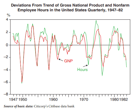
Let’s start with some basic results taken directly from Prescott’s paper. Figure $14.2$ shows log U.S. GDP and its trend. The trend is computed as a Hodrick-Prescott filter (think of this as a smoothed, but not fixed, line tracing the data). It is not a great way to compute the business cycle (particularly at the edges of the data set), but one that has become quite popular. Once the trend is computed, the cycle is easily estimated as the difference between the two and is showing in figure 14.3.

Figure $14.3$ also shows the variation over the cycle in hours worked. As you can see, there is a large positive correlation between the two.

Real business cycle papers will typically include a table with the properties of the economy, understood as the volatility of the variables and their cross-correlation over time. Table $14.1$ and $14.2$ show this from Prescott’s original paper for both the real data and the calibrated model.

As you can see, things work surprisingly well in the sense that most characteristics of the economy match. The volatility of output and the relative volatility of consumption and investment appear to be the optimal response to the supply shocks. The only caveat is that hours do not seem to move as much as in the data. This is why Prescott implemented Hansen’s extension. Figure $14.4$ shows how labour and output move in the Hansen economy (they seem to match better the pattern in Figure 14.1).
The Appendix to this chapter (at the end of the book) will walk you through an actual example so that you learn to numerically solve and simulate an RBC-style model yourself!

宏观经济学代考

经济代写|宏观经济学代写Macroeconomics代考|Calibration: An example

让我们考虑基本的 RBC 模型，以及 Prescott (1986) 提出的校准，这是该方法的实际启动，并且 Prescott 解决 了将参数分配给模型系数的问题。例如，当时，他持有 $\alpha=0.36^4$ 为了估计生产函数，他从我们反复使用的 Cobb-Douglas 规范开始
$$
f(k)=k^\alpha .
$$
请记住，利率必须等于资本的边际产量，
$$
f^{\prime}(k)=\alpha k^{\alpha-1},
$$
这意味着我们有一个资本回报率方程:
$$
r=\alpha \frac{Y}{K}-\delta .
$$
现在让我们给这个数字。什么是合理的折旧率? 让我们使用 (14.27) 本身来解决这个问题。如果我们假设折旧率 是 $10 \%$ 每年 (14.27) 变为
$$
0.04=0.36 \frac{Y}{K}-0.100 .14=0.36 \frac{Y}{K} \frac{0.36}{0.14}=\frac{K}{Y}=2.6
$$
资本产出率的这个值被认为是合理的，所以 $10 \%$ 折旧率似乎是一个合理的猜测。
折扣系数如何? 假设它等于利率。（这并不像看起来那么严格，但我们现在可以跳过它。）这意味着每年的贴现 率约为 $4 \%$ (实际利率)，所以 $\frac{1}{1+\rho}=0.96$ (再次，每年)。
至于跨期替代的弹性，他认为 $\sigma=1$ 是一个很好的近似值，并且使用的闲碬份额等于 $2 / 3$ ，正如我们所预期的 (这给出了一半的劳动力分配，如果我们认为可能的工作时间是每天 16 小时，这是合理的)。
最后，生产力冲击过程源自索洛剩余类型估计（正如我们在第 6 章讨论增长核算时所讨论的那样)，就当时的美 国而言，得出:
$$
z_{t+1}=0.9 * z_t+\varepsilon_{t+1^*}
$$
这是一个高度持久的过程，其中冲击具有非常持久的影响。扰动标准差的标定 $\varepsilon$ 是 $0.763$.
因此，有了所有这些参数，我们就可以将它们倒入规范中并随着时间的推移运行模型一一实际上，多次使用不同 的随机抽取来应对生产力冲击。这将在理论模型中给出经济的时间序列。现在，我们将看看这个经济的属性与实 体经济的属性相比如何。

经济代写|宏观经济学代写Macroeconomics代考|Does it work?

让我们从直接取自 Prescott 论文的一些基本结果开始。数字 $14.2$ 显示对数美国 GDP 及其趋势。趋势计算为 Hodrick-Prescott 滤波器 (将其视为平滑但不固定的跟踪数据的线)。这不是计算商业周期的好方法 (特别是在 数据集的边缘)，但它已经变得非常流行。一旦计算出趋势，周期很容易估计为两者之间的差异，如图 $14.3$ 所 示。
数字14.3还显示了以工作小时数为单位的周期变化。如您所见，两者之间存在很大的正相关。
真正的商业周期文件通常会包含一个包含经济属性的表格，即变量的波动性及其随时间的互相关性。桌子 $14.1$ 和14.2从 Prescott 的原始论文中展示了这一点，用于真实数据和校准模型。
正如你所看到的，在大多数经济特征相匹酛的意义上，事情运行得非常好。产出的波动以及消费和投资的相对波 动似乎是对供给冲击的最佳反应。唯一需要注意的是，小时数的变化似乎没有数据中的那么大。这就是 Prescott 实施 Hansen 扩展的原因。数字14.4显示了汉森经济中劳动力和产出如何变动（它们似乎更符合图 $14.1$ 中的模 式)。
本章的附录 (书末) 将引导您完成一个实际示例，以便您自己学习数值求解和模拟 RBC 样式的模型!

统计代写请认准statistics-lab™. statistics-lab™为您的留学生涯保驾护航。

金融工程代写

金融工程是使用数学技术来解决金融问题。金融工程使用计算机科学、统计学、经济学和应用数学领域的工具和知识来解决当前的金融问题，以及设计新的和创新的金融产品。

非参数统计代写

非参数统计指的是一种统计方法，其中不假设数据来自于由少数参数决定的规定模型；这种模型的例子包括正态分布模型和线性回归模型。

广义线性模型代考

广义线性模型（GLM）归属统计学领域，是一种应用灵活的线性回归模型。该模型允许因变量的偏差分布有除了正态分布之外的其它分布。

术语 广义线性模型（GLM）通常是指给定连续和/或分类预测因素的连续响应变量的常规线性回归模型。它包括多元线性回归，以及方差分析和方差分析（仅含固定效应）。

有限元方法代写

有限元方法（FEM）是一种流行的方法，用于数值解决工程和数学建模中出现的微分方程。典型的问题领域包括结构分析、传热、流体流动、质量运输和电磁势等传统领域。

有限元是一种通用的数值方法，用于解决两个或三个空间变量的偏微分方程（即一些边界值问题）。为了解决一个问题，有限元将一个大系统细分为更小、更简单的部分，称为有限元。这是通过在空间维度上的特定空间离散化来实现的，它是通过构建对象的网格来实现的：用于求解的数值域，它有有限数量的点。边界值问题的有限元方法表述最终导致一个代数方程组。该方法在域上对未知函数进行逼近。[1] 然后将模拟这些有限元的简单方程组合成一个更大的方程系统，以模拟整个问题。然后，有限元通过变化微积分使相关的误差函数最小化来逼近一个解决方案。

tatistics-lab作为专业的留学生服务机构，多年来已为美国、英国、加拿大、澳洲等留学热门地的学生提供专业的学术服务，包括但不限于Essay代写，Assignment代写，Dissertation代写，Report代写，小组作业代写，Proposal代写，Paper代写，Presentation代写，计算机作业代写，论文修改和润色，网课代做，exam代考等等。写作范围涵盖高中，本科，研究生等海外留学全阶段，辐射金融，经济学，会计学，审计学，管理学等全球99%专业科目。写作团队既有专业英语母语作者，也有海外名校硕博留学生，每位写作老师都拥有过硬的语言能力，专业的学科背景和学术写作经验。我们承诺100%原创，100%专业，100%准时，100%满意。

随机分析代写

随机微积分是数学的一个分支，对随机过程进行操作。它允许为随机过程的积分定义一个关于随机过程的一致的积分理论。这个领域是由日本数学家伊藤清在第二次世界大战期间创建并开始的。

时间序列分析代写

随机过程，是依赖于参数的一组随机变量的全体，参数通常是时间。 随机变量是随机现象的数量表现，其时间序列是一组按照时间发生先后顺序进行排列的数据点序列。通常一组时间序列的时间间隔为一恒定值（如1秒，5分钟，12小时，7天，1年），因此时间序列可以作为离散时间数据进行分析处理。研究时间序列数据的意义在于现实中，往往需要研究某个事物其随时间发展变化的规律。这就需要通过研究该事物过去发展的历史记录，以得到其自身发展的规律。

回归分析代写

多元回归分析渐进（Multiple Regression Analysis Asymptotics）属于计量经济学领域，主要是一种数学上的统计分析方法，可以分析复杂情况下各影响因素的数学关系，在自然科学、社会和经济学等多个领域内应用广泛。

MATLAB代写

MATLAB 是一种用于技术计算的高性能语言。它将计算、可视化和编程集成在一个易于使用的环境中，其中问题和解决方案以熟悉的数学符号表示。典型用途包括：数学和计算算法开发建模、仿真和原型制作数据分析、探索和可视化科学和工程图形应用程序开发，包括图形用户界面构建MATLAB 是一个交互式系统，其基本数据元素是一个不需要维度的数组。这使您可以解决许多技术计算问题，尤其是那些具有矩阵和向量公式的问题，而只需用 C 或 Fortran 等标量非交互式语言编写程序所需的时间的一小部分。MATLAB 名称代表矩阵实验室。MATLAB 最初的编写目的是提供对由 LINPACK 和 EISPACK 项目开发的矩阵软件的轻松访问，这两个项目共同代表了矩阵计算软件的最新技术。MATLAB 经过多年的发展，得到了许多用户的投入。在大学环境中，它是数学、工程和科学入门和高级课程的标准教学工具。在工业领域，MATLAB 是高效研究、开发和分析的首选工具。MATLAB 具有一系列称为工具箱的特定于应用程序的解决方案。对于大多数 MATLAB 用户来说非常重要，工具箱允许您学习和应用专业技术。工具箱是 MATLAB 函数（M 文件）的综合集合，可扩展 MATLAB 环境以解决特定类别的问题。可用工具箱的领域包括信号处理、控制系统、神经网络、模糊逻辑、小波、仿真等。

R语言代写	问卷设计与分析代写
PYTHON代写	回归分析与线性模型代写
MATLAB代写	方差分析与试验设计代写
STATA代写	机器学习/统计学习代写
SPSS代写	计量经济学代写
EVIEWS代写	时间序列分析代写
EXCEL代写	深度学习代写
SQL代写	各种数据建模与可视化代写

如果你也在 怎样代写宏观经济学Macroeconomics这个学科遇到相关的难题，请随时右上角联系我们的24/7代写客服。

宏观经济学，对国家或地区经济整体行为的研究。它关注的是了解整个经济的事件，如商品和服务的生产总量、失业水平和价格的一般行为。

statistics-lab™ 为您的留学生涯保驾护航 在代写宏观经济学Macroeconomics方面已经树立了自己的口碑, 保证靠谱, 高质且原创的统计Statistics代写服务。我们的专家在代写宏观经济学Macroeconomics代写方面经验极为丰富，各种代写宏观经济学Macroeconomics相关的作业也就用不着说。

我们提供的宏观经济学Macroeconomics及其相关学科的代写，服务范围广, 其中包括但不限于:

• Statistical Inference 统计推断
• Statistical Computing 统计计算
• Advanced Probability Theory 高等概率论
• Advanced Mathematical Statistics 高等数理统计学
• (Generalized) Linear Models 广义线性模型
• Statistical Machine Learning 统计机器学习
• Longitudinal Data Analysis 纵向数据分析
• Foundations of Data Science 数据科学基础

经济代写|宏观经济学代写Macroeconomics代考|The basic mechanics

In its essence, the RBC story goes as follows: consider a positive productivity shock that hits the economy, making it more productive. As a result of that shock, wages (i.e. MPL) and interest rates (i.e. MPK) go up, and individuals want to work more as a result. Because of that, output goes up. It follows that the elasticity of labour supply (and the closely related elasticity of intertemporal substitution) are crucial parameters for RBC models. One can only obtain large fluctuations in employment, as needed to match the data, if this elasticity is sufficiently high. What is the elasticity of labour supply in this basic model? Consider the case when $\frac{(i+r)}{(1+\rho)}=1$, in which consumption is a constant. We can read $(14.8)$ as implying a labour supply curve (a relation between $l_t$ and $w_t$ ):
$$
\phi v^{\prime}\left(1-l_t\right)=\lambda w_t,
$$

where $\lambda$ is the (constant) marginal utility of consumption. Let’s assume a slightly more general, functional form for the utility of leisure:
$$
v(h)=\frac{\sigma}{1-\sigma} h^{\frac{\sigma-1}{\sigma}},
$$
plugging this in (14.15) gives
$$
\phi h_{t^{-\frac{1}{0}}}=\lambda w_t
$$
or
$$
h_t=\left(\frac{\lambda w_t}{\phi}\right)^{-\sigma},
$$
which can be used to compute the labour supply:
$$
l_t=1-\left(\frac{\lambda w_t}{\phi}\right)^{-\sigma} .
$$
This equation has a labour supply elasticity in the short run equal to
$$
\frac{d l}{d w} \frac{w}{l}=\varepsilon_{l, w}=\frac{\sigma\left(\frac{\lambda w_t}{\phi}\right)^{-\sigma-1}\left(\frac{\lambda w_t}{\phi}\right)}{1-\left(\frac{\lambda w_t}{\phi}\right)^{-\sigma}}=\frac{\sigma\left(\frac{\lambda w_t}{\phi}\right)^{-\sigma}}{1-\left(\frac{\lambda w_t}{\phi}\right)^{-\sigma}}=\frac{\sigma h_t}{l_t}
$$
If we assume that $\sigma=1$ (logarithmic utility in leisure), and that $\phi$ and $\lambda$ are such that $\frac{h}{l}=2$ (think about an 8-hour workday), this gives you $\varepsilon_{l, w}=2$. This doesn’t seem to be enough to replicate the employment fluctuations observed in the data. On the other hand, it seems to be quite high if compared to micro data on the elasticity of labour supply. Do you think a decrease of $10 \%$ in real wages (because of inflation, for instance) would lead people to work $20 \%$ fewer hours?

经济代写|宏观经济学代写Macroeconomics代考|The indivisible labour solution

The RBC model thus delivers an elasticity of labour supply that is much higher than what micro evidence suggests, posing a challenge when it comes to matching real-world fluctuations in employment. One proposed solution for the conundrum is to incorporate the fact that labour decisions are often indivisible. This means that people may not make adjustments so much on the intensive margin of hôw mány hours to work in your joob, but moré oftenn on thẻ extensive margin of whéther to work at all. This implies that the aggregate elasticity is large even when the individual elasticity is small.

Hansen (1985) models that by assuming that there are fixed costs of going to work. This can actually make labour supply very responsive for a range of wage levels. The decision variables are both days of work: $d \leq \bar{d}$. and, then, the hours of work each day: $n$. We assume there is a fixed commuting cost in terms of utility $\kappa$, which you pay if you decide to work on that day, regardless of how many hours you work (this would be a sort of commuting time).

The objective function is now
$$
\operatorname{MaxE}\left[\sum_t\left(\frac{1}{1+\rho}\right)^t\left[u\left(c_t\right)-d_t v\left(n_t\right)-\kappa_t d_t\right]\right],
$$
where we leave aside the term $\phi$ to simplify notation, and abuse notation to have $v(\cdot)$ be a function of hours worked, rather than leisure, entering negatively in the utility function. The budget constraint is affected in that now wage income is equal to $w_t d_t n_t$.

It is easy to see that we have the same FOCs, (14.7) – which is unchanged because the terms in consumption in both maximand and budget constraint are still the same -, and (14.8) – because the term in $n_t$ is multiplied by $d_t$ in both maximand and budget constraint, so that $d_t$ cancels out. What changes is that now we have an extra FOC with respect to $d_t$ :
$$
\left[v\left(n_t\right)+k_t\right] \geq u^{\prime}\left(c_t\right) w_t n_t .
$$
Assume $\frac{(1+r)}{(1+\rho)}=1$, so that $c_t$ is constant. Then (14.8) simplifies to
$$
v^{\prime}\left(n_t\right)=\lambda w_t \Longrightarrow n^(w), $$ which gives the optimal amount of hours worked (when the agent decides to work). Then (14.22) simplifies to $$ v\left(n^\right)+k_t \geq \lambda w_t n^* .
$$
If $v\left(n^\right)+k>\lambda w n^$, then $d=0$, otherwise $d=\bar{d}$. This gives rise to a labour supply as shown in Figure $14.1$

The important point is that this labour supply curve is infinitely elastic at a certain wage. The intuition is that on the margin at which people decide whether to work at all or not, the labour supply will be very sensitive to changes in wages. ${ }^3$

宏观经济学代考

经济代写|宏观经济学代写Macroeconomics代考|The basic mechanics

从本质上讲，RBC 的故事如下：考虑对经济产生积极的生产力冲击，使其更具生产力。由于这种冲击，工资 (即 $\mathrm{MPL}$ ) 和利率 (即 MPK) 上升，因此个人希望工作更多。正因为如此，产量上升。由此可见，劳动力供给 的弹性 (以及密切相关的跨期替代弹性) 是 RBC 模型的关键参数。只有当这种弹性足够高时，才能获得与数据 匹配所需的就业大幅波动。在这个基本模型中，劳动力供给的弹性是多少? 考虑以下情况 $\frac{(i+r)}{(1+\rho)}=1$ ，其中消费 是一个常数。我们可以阅读 $(14.8)$ 作为暗示劳动力供给曲线 (之间的关系 $l_t$ 和 $w_t$ ):
$$
\phi v^{\prime}\left(1-l_t\right)=\lambda w_t,
$$
在哪里 $\lambda$ 是消费的 (不变的) 边际效用。让我们假设休闲效用的更一般的功能形式:
$$
v(h)=\frac{\sigma}{1-\sigma} h^{\frac{\sigma-1}{\sigma}},
$$
将其揷入 (14.15) 给出
$$
\phi h_{t-\frac{1}{0}}=\lambda w_t
$$
或者
$$
h_t=\left(\frac{\lambda w_t}{\phi}\right)^{-\sigma}
$$
可用于计算劳动力供给：
$$
l_t=1-\left(\frac{\lambda w_t}{\phi}\right)^{-\sigma}
$$
这个方程的短期劳动力供给弹性等于
$$
\frac{d l}{d w} \frac{w}{l}=\varepsilon_{l, w}=\frac{\sigma\left(\frac{\lambda w_t}{\phi}\right)^{-\sigma-1}\left(\frac{\lambda w_t}{\phi}\right)}{1-\left(\frac{\lambda w_t}{\phi}\right)^{-\sigma}}=\frac{\sigma\left(\frac{\lambda w_t}{\phi}\right)^{-\sigma}}{1-\left(\frac{\lambda w_t}{\phi}\right)^{-\sigma}}=\frac{\sigma h_t}{l_t}
$$
如果我们假设 $\sigma=1$ (休闲中的对数效用)，并且 $\phi$ 和 $\lambda$ 是这样的 $\frac{h}{l}=2$ (想想一个 8 小时的工作日) ，这给了 你 $\varepsilon_{l, w}=2$. 这似乎不足以复制数据中观察到的就业波动。另一方面，如果与劳动力供给弹性的微观数据相比， 它似乎相当高。你认为减少 $10 \%$ 实际工资（例如，由于通货膨胀) 会导致人们工作 $20 \%$ 更少的时间?

经济代写|宏观经济学代写Macroeconomics代考|The indivisible labour solution

因此，RBC 模型提供的劳动力供给弹性远高于微观证据表明的水平，这在匹配现实世界的就业波动方面提出了 挑战。解决这个难题的一种建议是将劳动决策通常是不可分割的事实结合起来。这意味着人们可能不会在你的工 作中工作多少小时的密集边际上做出太多调整，但更经常地在是否工作的广泛边际上做出调整。这意味着即使个 体弹性很小，总体弹性也很大。

Hansen (1985) 通过假设上班有固定成本来建模。这实际上可以使劳动力供应对一系列工资水平非常敏感。决策 变量都是工作天数： $d \leq \bar{d}$. 然后是每天的工作时间： $n$. 我们假设在公用事业方面存在固定的通勤成本 $\kappa$ ，如果 您决定在那一天工作，无论您工作多少小时（这将是一种通勤时间），您都需要支付这笔费用。
现在的目标函数是
$$
\operatorname{MaxE}\left[\sum_t\left(\frac{1}{1+\rho}\right)^t\left[u\left(c_t\right)-d_t v\left(n_t\right)-\kappa_t d_t\right]\right]
$$
我们把这个词放在一边 $\phi$ 简化符号，滥用符号 $v(\cdot)$ 是工作时间的函数，而不是休闲时间，在效用函数中为负数。 预算约束受到影响，因为现在工资收入等于 $w_t d_t n_t$.
很容易看出，我们有相同的 FOC，(14.7) —一它没有改变，因为最大值和预算约束中的消费项仍然相同一— 和 (14.8) —一因为在 $n_t$ 乘以 $d_t$ 在最大约束和预算约束中，所以 $d_t$ 取消。改变的是现在我们有一个额外的 FOC $d_t$ :
$$
\left[v\left(n_t\right)+k_t\right] \geq u^{\prime}\left(c_t\right) w_t n_t
$$
认为 $\frac{(1+r)}{(1+\rho)}=1$ ，以便 $c_t$ 是恒定的。那么 (14.8) 简化为
$$
\left.v^{\prime}\left(n_t\right)=\lambda w_t \Longrightarrow n^{(} w\right)
$$
这给出了最佳的工作时间 (当代理决定工作时)。那么 (14.22) 简化为
vleft(n^1right)+k_t lgeq \ambda w_t $n^{n^{\star}}$ 。
如果 $\vee \backslash l e f t\left(\mathrm{n}^{\wedge} \backslash \mathrm{right}\right)+\mathrm{k}>\backslash \mathrm{ambda} \mathrm{w} \mathrm{n}^{\wedge}$ ， 然后 $d=0$ ，否则 $d=\bar{d}$. 这产生了如图所示的劳动力供给 $14.1$
重要的一点是，在一定工资条件下，这条劳动力供给曲线是无限弹性的。直觉是，在人们决定是否工作的边际 上，劳动力供应将对工资的变化非常敏感。

统计代写请认准statistics-lab™. statistics-lab™为您的留学生涯保驾护航。

金融工程代写

金融工程是使用数学技术来解决金融问题。金融工程使用计算机科学、统计学、经济学和应用数学领域的工具和知识来解决当前的金融问题，以及设计新的和创新的金融产品。

非参数统计代写

非参数统计指的是一种统计方法，其中不假设数据来自于由少数参数决定的规定模型；这种模型的例子包括正态分布模型和线性回归模型。

广义线性模型代考

广义线性模型（GLM）归属统计学领域，是一种应用灵活的线性回归模型。该模型允许因变量的偏差分布有除了正态分布之外的其它分布。

术语 广义线性模型（GLM）通常是指给定连续和/或分类预测因素的连续响应变量的常规线性回归模型。它包括多元线性回归，以及方差分析和方差分析（仅含固定效应）。

有限元方法代写

有限元方法（FEM）是一种流行的方法，用于数值解决工程和数学建模中出现的微分方程。典型的问题领域包括结构分析、传热、流体流动、质量运输和电磁势等传统领域。

有限元是一种通用的数值方法，用于解决两个或三个空间变量的偏微分方程（即一些边界值问题）。为了解决一个问题，有限元将一个大系统细分为更小、更简单的部分，称为有限元。这是通过在空间维度上的特定空间离散化来实现的，它是通过构建对象的网格来实现的：用于求解的数值域，它有有限数量的点。边界值问题的有限元方法表述最终导致一个代数方程组。该方法在域上对未知函数进行逼近。[1] 然后将模拟这些有限元的简单方程组合成一个更大的方程系统，以模拟整个问题。然后，有限元通过变化微积分使相关的误差函数最小化来逼近一个解决方案。

tatistics-lab作为专业的留学生服务机构，多年来已为美国、英国、加拿大、澳洲等留学热门地的学生提供专业的学术服务，包括但不限于Essay代写，Assignment代写，Dissertation代写，Report代写，小组作业代写，Proposal代写，Paper代写，Presentation代写，计算机作业代写，论文修改和润色，网课代做，exam代考等等。写作范围涵盖高中，本科，研究生等海外留学全阶段，辐射金融，经济学，会计学，审计学，管理学等全球99%专业科目。写作团队既有专业英语母语作者，也有海外名校硕博留学生，每位写作老师都拥有过硬的语言能力，专业的学科背景和学术写作经验。我们承诺100%原创，100%专业，100%准时，100%满意。

随机分析代写

随机微积分是数学的一个分支，对随机过程进行操作。它允许为随机过程的积分定义一个关于随机过程的一致的积分理论。这个领域是由日本数学家伊藤清在第二次世界大战期间创建并开始的。

时间序列分析代写

随机过程，是依赖于参数的一组随机变量的全体，参数通常是时间。 随机变量是随机现象的数量表现，其时间序列是一组按照时间发生先后顺序进行排列的数据点序列。通常一组时间序列的时间间隔为一恒定值（如1秒，5分钟，12小时，7天，1年），因此时间序列可以作为离散时间数据进行分析处理。研究时间序列数据的意义在于现实中，往往需要研究某个事物其随时间发展变化的规律。这就需要通过研究该事物过去发展的历史记录，以得到其自身发展的规律。

回归分析代写

多元回归分析渐进（Multiple Regression Analysis Asymptotics）属于计量经济学领域，主要是一种数学上的统计分析方法，可以分析复杂情况下各影响因素的数学关系，在自然科学、社会和经济学等多个领域内应用广泛。

MATLAB代写

MATLAB 是一种用于技术计算的高性能语言。它将计算、可视化和编程集成在一个易于使用的环境中，其中问题和解决方案以熟悉的数学符号表示。典型用途包括：数学和计算算法开发建模、仿真和原型制作数据分析、探索和可视化科学和工程图形应用程序开发，包括图形用户界面构建MATLAB 是一个交互式系统，其基本数据元素是一个不需要维度的数组。这使您可以解决许多技术计算问题，尤其是那些具有矩阵和向量公式的问题，而只需用 C 或 Fortran 等标量非交互式语言编写程序所需的时间的一小部分。MATLAB 名称代表矩阵实验室。MATLAB 最初的编写目的是提供对由 LINPACK 和 EISPACK 项目开发的矩阵软件的轻松访问，这两个项目共同代表了矩阵计算软件的最新技术。MATLAB 经过多年的发展，得到了许多用户的投入。在大学环境中，它是数学、工程和科学入门和高级课程的标准教学工具。在工业领域，MATLAB 是高效研究、开发和分析的首选工具。MATLAB 具有一系列称为工具箱的特定于应用程序的解决方案。对于大多数 MATLAB 用户来说非常重要，工具箱允许您学习和应用专业技术。工具箱是 MATLAB 函数（M 文件）的综合集合，可扩展 MATLAB 环境以解决特定类别的问题。可用工具箱的领域包括信号处理、控制系统、神经网络、模糊逻辑、小波、仿真等。

R语言代写	问卷设计与分析代写
PYTHON代写	回归分析与线性模型代写
MATLAB代写	方差分析与试验设计代写
STATA代写	机器学习/统计学习代写
SPSS代写	计量经济学代写
EVIEWS代写	时间序列分析代写
EXCEL代写	深度学习代写
SQL代写	各种数据建模与可视化代写

如果你也在 怎样代写宏观经济学Macroeconomics这个学科遇到相关的难题，请随时右上角联系我们的24/7代写客服。

宏观经济学，对国家或地区经济整体行为的研究。它关注的是了解整个经济的事件，如商品和服务的生产总量、失业水平和价格的一般行为。

statistics-lab™ 为您的留学生涯保驾护航 在代写宏观经济学Macroeconomics方面已经树立了自己的口碑, 保证靠谱, 高质且原创的统计Statistics代写服务。我们的专家在代写宏观经济学Macroeconomics代写方面经验极为丰富，各种代写宏观经济学Macroeconomics相关的作业也就用不着说。

我们提供的宏观经济学Macroeconomics及其相关学科的代写，服务范围广, 其中包括但不限于:

• Statistical Inference 统计推断
• Statistical Computing 统计计算
• Advanced Probability Theory 高等概率论
• Advanced Mathematical Statistics 高等数理统计学
• (Generalized) Linear Models 广义线性模型
• Statistical Machine Learning 统计机器学习
• Longitudinal Data Analysis 纵向数据分析
• Foundations of Data Science 数据科学基础

经济代写|宏观经济学代写Macroeconomics代考|The importance of labour supply

As we’ve pointed out, one of the RBC literature’s main departures from the standard NGM is the presence of a labour supply choice. This is crucial to generate fluctuations in employment, which are a pervasive feature of actual business cycles. Let us consider this choice within the context of the basic model. With log utility, the consumer’s objective function can be thought of as:
$$
E\left[\sum_t\left(\frac{1}{1+\rho}\right)^t\left[(1-\phi) \log \left(c_t\right)+\phi \log \left(h_t\right)\right] .\right.
$$
Notice that the household has two control variables, consumption and leisure. We have seen before the solution to the problem of optimal intertemporal allocation of consumption; it is the familiar Euler equation:
$$
u^{\prime}\left(c_t\right)=\frac{1+r_{t+1}}{1+\rho} E\left[u^{\prime}\left(c_{t+1}\right)\right] .
$$
Leaving aside uncertainty, for the moment, and using the log assumption, we can rewrite this as:
$$
c_{t+1}=\frac{1+r_{t+1}}{1+\rho} c_t .
$$
The labour-leisure choice, in contrast, is static; it takes place in each period with no implication for the next period. The FOC equates the marginal benefit of additional consumption to the marginal cost of lost leisure:
$$
w_t(1-\phi) u^{\prime}\left(c_t\right)=\phi v^{\prime}\left(h_t\right) .
$$
Again using the log utility assumption, we get
$$
w_t(1-\phi) h_t=\phi c_t .
$$
To simplify things further, assume for the moment that $r$ is exogenous – think of a small open economy. In this setup, we can use (14.9) into (14.7) to obtain
$$
\frac{h_{t+1}}{h_t}=\frac{1+r}{1+\rho} \frac{w_t}{w_{t+1}} \Rightarrow \frac{1-l_{t+1}}{1-l_t}=\frac{1+r}{1+\rho} \frac{w_t}{w_{t+1}} .
$$
This means that leisure will be relatively high in those periods when the wage is relatively low; in other words, a higher wage increases the supply of labour. We can also see the impact of the interest rate: a high interest rate will lead to a higher supply of labour. The intuition is that it is worth working more in the present the higher the interest rate, as it provides a higher return in terms of future leisure. These responses of the labour supply, driven by intertemporal substitution in labour and leisure, are at the very heart of the fluctuations in employment in RBC models.

经济代写|宏观经济学代写Macroeconomics代考|The long-run labour supply

Let’s pause for a minute to explore a bit deeper the shape of this labour supply curve. Consider the case when wages and income are constant, a case that would be akin to analysing the effect of permanent shocks to these variables. Let’s see the form of the labour supply in this case.

Since consumption is constant at income level
$$
c_t=w\left(1-h_t\right)
$$
substituting this into (14.8) we obtain
$$
(1-\phi) u^{\prime}\left(w\left(1-h_t\right)\right)=\frac{\phi v^{\prime}\left(h_t\right)}{w}
$$
Using the log specification for consumption and allowing for $\phi=\frac{2}{3}$ allows us to simplify
$$
\left(\frac{1}{3}\right) \frac{1}{w\left(1-h_t\right)}=\frac{2}{3} \frac{1}{w h_t}
$$
This is a strong result that says that leisure is independent of the wage level. You may think this is too strong but, surprisingly, it fits the data very well, at least when thinking about labour supply in the very, very long run. ${ }^2$ It does seem that for humans income and substitution effects just cancel out (or maybe you prefer a more Leontieff setup in which people just can’t work more than eight hours per day, or where the disutility of labour beyond eight hours a day becomes unbearable if repeated every day).
Does this mean that labour supply does not move at all? Not really. The above was derived under the assumption of the constancy of the wage. This is akin to assuming that any change in wages is permanent, which induces a very large response in the shadow value of consumption that works to offset the labour supply effect of the change in wages (totally cancelling it in the log case). But if the wage moves for a very short period of time we can assume the shadow value of consumption to remain constant, and then changes in the wage will elicit a labour supply response. Thus, while the long-run elasticity of labour supply may be zero, it is positive in the short run.

宏观经济学代考

经济代写|宏观经济学代写Macroeconomics代考|The importance of labour supply

正如我们所指出的，RBC 文献与标准 NGM 的主要区别之一是存在劳动力供应选择。这对于产生就业波动至关重 要，这是实际商业周期的普遍特征。让我们在基本模型的背景下考虑这个选择。使用 log 实用程序，消费者的目 标函数可以被认为是:
$$
E\left[\sum_t\left(\frac{1}{1+\rho}\right)^t\left[(1-\phi) \log \left(c_t\right)+\phi \log \left(h_t\right)\right] .\right.
$$
请注意，家庭有两个控制变量，消费和休闲。我们之前已经看到了消费跨期最优分配问题的解决方案；这是熟悉 的欧拉方程:
$$
u^{\prime}\left(c_t\right)=\frac{1+r_{t+1}}{1+\rho} E\left[u^{\prime}\left(c_{t+1}\right)\right] .
$$
暂时不考虑不确定性，并使用对数假设，我们可以将其重写为:
$$
c_{t+1}=\frac{1+r_{t+1}}{1+\rho} c_t .
$$
相比之下，劳动休闲选择是静态的。它发生在每个时期，对下一个时期没有影响。FOC 将额外消费的边际收益 等同于失去休闲的边际成本:
$$
w_t(1-\phi) u^{\prime}\left(c_t\right)=\phi v^{\prime}\left(h_t\right) .
$$
再次使用 $\log$ 效用假设，我们得到
$$
w_t(1-\phi) h_t=\phi c_t .
$$
为了进一步简化事情，暂时假设 $r$ 是外生的一一想想一个小型的开放经济。在这个设置中，我们可以使用 (14.9) 到 (14.7) 来获得
$$
\frac{h_{t+1}}{h_t}=\frac{1+r}{1+\rho} \frac{w_t}{w_{t+1}} \Rightarrow \frac{1-l_{t+1}}{1-l_t}=\frac{1+r}{1+\rho} \frac{w_t}{w_{t+1}} .
$$
这意味着在工资相对较低的时期，闲暇时间会相对较高；换句话说，更高的工资会增加劳动力的供应。我们还可 以看到利率的影响: 高利率会导致更高的劳动力供应。直觉是，利率越高，现在越值得工作，因为它在末来的休 闲方面提供了更高的回报。这些由劳动力和休闲的跨期替代驱动的劳动力供应反应是 RBC 模型中就业波动的核 心。

经济代写|宏观经济学代写Macroeconomics代考|The long-run labour supply

让我们暂停一分钟，更深入地探讨一下这条劳动力供给曲线的形状。考虑工资和收入不变的情况，这种情况类似 于分析永久性冲击对这些变量的影响。让我们看看这种情况下的劳动力供给形式。
由于消费在收入水平上是恒定的
$$
c_t=w\left(1-h_t\right)
$$
将其代入 (14.8) 我们得到
$$
(1-\phi) u^{\prime}\left(w\left(1-h_t\right)\right)=\frac{\phi v^{\prime}\left(h_t\right)}{w}
$$
使用日志规范进行消费并允许 $\phi=\frac{2}{3}$ 允许我们简化
$$
\left(\frac{1}{3}\right) \frac{1}{w\left(1-h_t\right)}=\frac{2}{3} \frac{1}{w h_t}
$$
这是一个强有力的结果，表明休闲与工资水平无关。你可能认为这太强了，但令人惊讶的是，它非常符合数据， 至少在考虑非常非常长期的劳动力供应时。 ${ }^2$ 对于人类而言，收入和替代效应似乎确实抵消了 (或者您可能更喜 欢 Leontieff 设置，在这种设置中，人们每天工作不能超过八小时，或者一天超过八小时的劳动无用性变得难以 忍受如果每天重复)。
这是否意味着劳动力供给根本不动? 并不真地。以上是在工资不变的假设下得出的。这类似于假设工资的任何变 化都是永久性的，这会引起诮费影子价值的非常大的反应，从而抵消工资变化的劳动力供给效应（在对数情况下 完全抵峭)。但如果工资在很短的时间内变动，我们可以假设消费的影子价值保持不变，然后工资的变化将引发 劳动力供给反应。因此，虽然劳动力供给的长期弹性可能为零，但在短期内是正的。

统计代写请认准statistics-lab™. statistics-lab™为您的留学生涯保驾护航。

金融工程代写

金融工程是使用数学技术来解决金融问题。金融工程使用计算机科学、统计学、经济学和应用数学领域的工具和知识来解决当前的金融问题，以及设计新的和创新的金融产品。

非参数统计代写

非参数统计指的是一种统计方法，其中不假设数据来自于由少数参数决定的规定模型；这种模型的例子包括正态分布模型和线性回归模型。

广义线性模型代考

广义线性模型（GLM）归属统计学领域，是一种应用灵活的线性回归模型。该模型允许因变量的偏差分布有除了正态分布之外的其它分布。

术语 广义线性模型（GLM）通常是指给定连续和/或分类预测因素的连续响应变量的常规线性回归模型。它包括多元线性回归，以及方差分析和方差分析（仅含固定效应）。

有限元方法代写

有限元方法（FEM）是一种流行的方法，用于数值解决工程和数学建模中出现的微分方程。典型的问题领域包括结构分析、传热、流体流动、质量运输和电磁势等传统领域。

有限元是一种通用的数值方法，用于解决两个或三个空间变量的偏微分方程（即一些边界值问题）。为了解决一个问题，有限元将一个大系统细分为更小、更简单的部分，称为有限元。这是通过在空间维度上的特定空间离散化来实现的，它是通过构建对象的网格来实现的：用于求解的数值域，它有有限数量的点。边界值问题的有限元方法表述最终导致一个代数方程组。该方法在域上对未知函数进行逼近。[1] 然后将模拟这些有限元的简单方程组合成一个更大的方程系统，以模拟整个问题。然后，有限元通过变化微积分使相关的误差函数最小化来逼近一个解决方案。

tatistics-lab作为专业的留学生服务机构，多年来已为美国、英国、加拿大、澳洲等留学热门地的学生提供专业的学术服务，包括但不限于Essay代写，Assignment代写，Dissertation代写，Report代写，小组作业代写，Proposal代写，Paper代写，Presentation代写，计算机作业代写，论文修改和润色，网课代做，exam代考等等。写作范围涵盖高中，本科，研究生等海外留学全阶段，辐射金融，经济学，会计学，审计学，管理学等全球99%专业科目。写作团队既有专业英语母语作者，也有海外名校硕博留学生，每位写作老师都拥有过硬的语言能力，专业的学科背景和学术写作经验。我们承诺100%原创，100%专业，100%准时，100%满意。

随机分析代写

随机微积分是数学的一个分支，对随机过程进行操作。它允许为随机过程的积分定义一个关于随机过程的一致的积分理论。这个领域是由日本数学家伊藤清在第二次世界大战期间创建并开始的。

时间序列分析代写

随机过程，是依赖于参数的一组随机变量的全体，参数通常是时间。 随机变量是随机现象的数量表现，其时间序列是一组按照时间发生先后顺序进行排列的数据点序列。通常一组时间序列的时间间隔为一恒定值（如1秒，5分钟，12小时，7天，1年），因此时间序列可以作为离散时间数据进行分析处理。研究时间序列数据的意义在于现实中，往往需要研究某个事物其随时间发展变化的规律。这就需要通过研究该事物过去发展的历史记录，以得到其自身发展的规律。

回归分析代写

多元回归分析渐进（Multiple Regression Analysis Asymptotics）属于计量经济学领域，主要是一种数学上的统计分析方法，可以分析复杂情况下各影响因素的数学关系，在自然科学、社会和经济学等多个领域内应用广泛。

MATLAB代写

MATLAB 是一种用于技术计算的高性能语言。它将计算、可视化和编程集成在一个易于使用的环境中，其中问题和解决方案以熟悉的数学符号表示。典型用途包括：数学和计算算法开发建模、仿真和原型制作数据分析、探索和可视化科学和工程图形应用程序开发，包括图形用户界面构建MATLAB 是一个交互式系统，其基本数据元素是一个不需要维度的数组。这使您可以解决许多技术计算问题，尤其是那些具有矩阵和向量公式的问题，而只需用 C 或 Fortran 等标量非交互式语言编写程序所需的时间的一小部分。MATLAB 名称代表矩阵实验室。MATLAB 最初的编写目的是提供对由 LINPACK 和 EISPACK 项目开发的矩阵软件的轻松访问，这两个项目共同代表了矩阵计算软件的最新技术。MATLAB 经过多年的发展，得到了许多用户的投入。在大学环境中，它是数学、工程和科学入门和高级课程的标准教学工具。在工业领域，MATLAB 是高效研究、开发和分析的首选工具。MATLAB 具有一系列称为工具箱的特定于应用程序的解决方案。对于大多数 MATLAB 用户来说非常重要，工具箱允许您学习和应用专业技术。工具箱是 MATLAB 函数（M 文件）的综合集合，可扩展 MATLAB 环境以解决特定类别的问题。可用工具箱的领域包括信号处理、控制系统、神经网络、模糊逻辑、小波、仿真等。

R语言代写	问卷设计与分析代写
PYTHON代写	回归分析与线性模型代写
MATLAB代写	方差分析与试验设计代写
STATA代写	机器学习/统计学习代写
SPSS代写	计量经济学代写
EVIEWS代写	时间序列分析代写
EXCEL代写	深度学习代写
SQL代写	各种数据建模与可视化代写

如果你也在 怎样代写宏观经济学Macroeconomics这个学科遇到相关的难题，请随时右上角联系我们的24/7代写客服。

宏观经济学，对国家或地区经济整体行为的研究。它关注的是了解整个经济的事件，如商品和服务的生产总量、失业水平和价格的一般行为。

statistics-lab™ 为您的留学生涯保驾护航 在代写宏观经济学Macroeconomics方面已经树立了自己的口碑, 保证靠谱, 高质且原创的统计Statistics代写服务。我们的专家在代写宏观经济学Macroeconomics代写方面经验极为丰富，各种代写宏观经济学Macroeconomics相关的作业也就用不着说。

我们提供的宏观经济学Macroeconomics及其相关学科的代写，服务范围广, 其中包括但不限于:

• Statistical Inference 统计推断
• Statistical Computing 统计计算
• Advanced Probability Theory 高等概率论
• Advanced Mathematical Statistics 高等数理统计学
• (Generalized) Linear Models 广义线性模型
• Statistical Machine Learning 统计机器学习
• Longitudinal Data Analysis 纵向数据分析
• Foundations of Data Science 数据科学基础

经济代写|宏观经济学代写Macroeconomics代考|The dynamics of technology, education and population

In order to close the picture, we need to have a model of how technological progress takes place. Inspired by the models of endogenous growth that we have seen, we think of productivity growth being driven by the accumulation of knowledge, which is enhanced by human capital and by scale effects. Quite simply, we posit
$$
g_{t+1} \equiv \frac{A_{t+1}-A_t}{A_t}=g\left(e_t, L_t\right),
$$
where $g(\cdot, \cdot)$ is increasing and concave in both arguments: more and more educated people increase the rate of growth, at decreasing rates. (Remember that our discussion of scale effects argued that there is good evidence for their presence in this very long-run context, as per the models of innovation studied in Chapter 6 and synthesised in Kremer (1993).)

Obviously, the evolution of the size of the adult population is described by $L_{t+1}=n_t L_t$, since $n_t$ is the number of children that each individual adult alive at time $t$ chooses to have. The model of demographic decisions shows that $n_t$ is a function of the rate of technological progress and, when the subsistence constraint is binding, also of potential income. Potential income, in turn, is a function of the existing technology, education levels, and the amount of effective resources per worker.

The one thing that is missing is the evolution of potential resources per worker, $x_t \equiv \frac{A_t X}{L_t}$, but that is easy to state: $x_{t+1}=\frac{1+g_{t+1}}{n_t} x_t$, that is, effective resources per worker grow at the rate of productivity, adjusted by the growth of population.

We now have a dynamic system in four variables: $g_t, x_t, e_t$, and $L_t$. These capture all of our variables of interest, namely productivity growth, productivity levels, human capital investment, and population.

经济代写|宏观经济学代写Macroeconomics代考|The full picture

Figure $10.5$ encompasses all of our story, from the Malthusian regime to sustained growth. Consider an economy in early stages of development. Population size is relatively small and the implied slow rate of technological progress does not provide an incentive to invest in the education of children: this is the world of Figure $10.5 \mathrm{~A}$ – the Malthusian Regime. Over time, the slow growth in population that takes place in the Malthusian Regime raises the rate of technological progress and shifts the $g$ in Panel A enough to generate a qualitative change to Panel B. This is characterised by multiple, historydependent, stable steady-state equilibria: some countries may take off and start investing in human capital, while others lag behind. However, since the economy started in the Malthusian steady state, it initially sticks in the vicinity of that steady state, which is still stable in the absence of major shocks.
Eventually, the continued increase in population leads us to Panel $\mathrm{C}$ : the Malthusian steady state disappears, and the economy starts converging to the steady state with high education. The resulting increase in the pace of technological progress, due to the increased levels of education, has two opposing effects on the evolution of population. On the one hand, it allows for the allocation of more resources for raising children. On the other hand, it induces a reallocation of these additional resources toward child quality. Initially, there is low demand for human capital, and the first effect dominates: this is the Post-Malthusian Regime.

The interaction between investment in human capital and technological progress generates a virtuous circle: human capital formation pushes faster technological progress, which further raises the demand for human capital, which fosters more investment in child quality. Eventually, the subsistence constraint seizes to bind, triggering a demographic transition and sustained economic growth.

宏观经济学代考

经济代写|宏观经济学代写宏观经济学代考|技术、教育和人口的动态

为了结束这幅图，我们需要有一个技术进步是如何发生的模型。受我们所见过的内生增长模型的启发，我们认为生产力增长是由知识积累驱动的，而知识积累又由人力资本和规模效应增强。很简单，我们假定
$$
g_{t+1} \equiv \frac{A_{t+1}-A_t}{A_t}=g\left(e_t, L_t\right),
$$
，其中$g(\cdot, \cdot)$在两个论证中都是递增和凹的:越来越多受教育的人增加了增长率，但增长率在下降。(请记住，我们对规模效应的讨论认为，在这个非常长期的背景下，有很好的证据证明它们的存在，根据第六章研究的创新模型，并由Kremer(1993)综合。

显然，成人人口规模的演变可以用$L_{t+1}=n_t L_t$来描述，因为$n_t$是$t$时期每个活着的成年人选择生育的子女数量。人口决策模型表明，$n_t$是技术进步速度的函数，当生存限制具有约束力时，也是潜在收入的函数。反过来，潜在收入是现有技术、教育水平和每个工人的有效资源量的函数

唯一缺少的是每个工人潜在资源的演化，$x_t \equiv \frac{A_t X}{L_t}$，但这很容易表述:$x_{t+1}=\frac{1+g_{t+1}}{n_t} x_t$，也就是说，每个工人的有效资源以生产力的速度增长，由人口的增长调整

我们现在有一个包含四个变量的动态系统:$g_t, x_t, e_t$和$L_t$。这些涵盖了我们感兴趣的所有变量，即生产力增长、生产力水平、人力资本投资和人口

经济代写|宏观经济学代写宏观经济代考|全图

图$10.5$包含了我们所有的故事，从马尔萨斯制度到持续增长。考虑一个处于发展早期阶段的经济体。人口规模相对较小，隐含的技术进步的缓慢速度并不能提供对儿童教育投资的激励:这就是图$10.5 \mathrm{~A}$中的世界-马尔萨斯制度。随着时间的推移，马尔萨斯体制中发生的人口缓慢增长提高了技术进步的速度，并将A组中的$g$转移到b组，从而产生质变。这一过程的特征是多重的、依赖历史的、稳定的稳态均衡:一些国家可能起飞并开始投资人力资本，而另一些国家则落后于b组。然而，由于经济是从马尔萨斯稳态开始的，它最初停留在稳态附近，在没有重大冲击的情况下，该稳态仍然是稳定的。最终，人口的持续增长把我们带到了版块$\mathrm{C}$:马尔萨斯稳态消失了，经济开始收敛到有高等教育的稳态。由于教育水平的提高而导致的技术进步速度的加快，对人口的演变产生了两种相反的影响。一方面，它允许分配更多的资源来抚养孩子。另一方面，它导致这些额外的资源重新分配到孩子的素质上。最初，对人力资本的需求较低，第一种效应占主导地位:这是后马尔萨斯制度

人力资本投资与技术进步的相互作用形成了一个良性循环:人力资本的形成推动技术进步的加快，技术进步进一步提高了对人力资本的需求，从而促进了对儿童素质的更多投资。最终，生存限制开始起作用，引发人口转型和持续的经济增长

统计代写请认准statistics-lab™. statistics-lab™为您的留学生涯保驾护航。

金融工程代写

金融工程是使用数学技术来解决金融问题。金融工程使用计算机科学、统计学、经济学和应用数学领域的工具和知识来解决当前的金融问题，以及设计新的和创新的金融产品。

非参数统计代写

非参数统计指的是一种统计方法，其中不假设数据来自于由少数参数决定的规定模型；这种模型的例子包括正态分布模型和线性回归模型。

广义线性模型代考

广义线性模型（GLM）归属统计学领域，是一种应用灵活的线性回归模型。该模型允许因变量的偏差分布有除了正态分布之外的其它分布。

术语 广义线性模型（GLM）通常是指给定连续和/或分类预测因素的连续响应变量的常规线性回归模型。它包括多元线性回归，以及方差分析和方差分析（仅含固定效应）。

有限元方法代写

有限元方法（FEM）是一种流行的方法，用于数值解决工程和数学建模中出现的微分方程。典型的问题领域包括结构分析、传热、流体流动、质量运输和电磁势等传统领域。

有限元是一种通用的数值方法，用于解决两个或三个空间变量的偏微分方程（即一些边界值问题）。为了解决一个问题，有限元将一个大系统细分为更小、更简单的部分，称为有限元。这是通过在空间维度上的特定空间离散化来实现的，它是通过构建对象的网格来实现的：用于求解的数值域，它有有限数量的点。边界值问题的有限元方法表述最终导致一个代数方程组。该方法在域上对未知函数进行逼近。[1] 然后将模拟这些有限元的简单方程组合成一个更大的方程系统，以模拟整个问题。然后，有限元通过变化微积分使相关的误差函数最小化来逼近一个解决方案。

tatistics-lab作为专业的留学生服务机构，多年来已为美国、英国、加拿大、澳洲等留学热门地的学生提供专业的学术服务，包括但不限于Essay代写，Assignment代写，Dissertation代写，Report代写，小组作业代写，Proposal代写，Paper代写，Presentation代写，计算机作业代写，论文修改和润色，网课代做，exam代考等等。写作范围涵盖高中，本科，研究生等海外留学全阶段，辐射金融，经济学，会计学，审计学，管理学等全球99%专业科目。写作团队既有专业英语母语作者，也有海外名校硕博留学生，每位写作老师都拥有过硬的语言能力，专业的学科背景和学术写作经验。我们承诺100%原创，100%专业，100%准时，100%满意。

随机分析代写

随机微积分是数学的一个分支，对随机过程进行操作。它允许为随机过程的积分定义一个关于随机过程的一致的积分理论。这个领域是由日本数学家伊藤清在第二次世界大战期间创建并开始的。

时间序列分析代写

随机过程，是依赖于参数的一组随机变量的全体，参数通常是时间。 随机变量是随机现象的数量表现，其时间序列是一组按照时间发生先后顺序进行排列的数据点序列。通常一组时间序列的时间间隔为一恒定值（如1秒，5分钟，12小时，7天，1年），因此时间序列可以作为离散时间数据进行分析处理。研究时间序列数据的意义在于现实中，往往需要研究某个事物其随时间发展变化的规律。这就需要通过研究该事物过去发展的历史记录，以得到其自身发展的规律。

回归分析代写

多元回归分析渐进（Multiple Regression Analysis Asymptotics）属于计量经济学领域，主要是一种数学上的统计分析方法，可以分析复杂情况下各影响因素的数学关系，在自然科学、社会和经济学等多个领域内应用广泛。

MATLAB代写

MATLAB 是一种用于技术计算的高性能语言。它将计算、可视化和编程集成在一个易于使用的环境中，其中问题和解决方案以熟悉的数学符号表示。典型用途包括：数学和计算算法开发建模、仿真和原型制作数据分析、探索和可视化科学和工程图形应用程序开发，包括图形用户界面构建MATLAB 是一个交互式系统，其基本数据元素是一个不需要维度的数组。这使您可以解决许多技术计算问题，尤其是那些具有矩阵和向量公式的问题，而只需用 C 或 Fortran 等标量非交互式语言编写程序所需的时间的一小部分。MATLAB 名称代表矩阵实验室。MATLAB 最初的编写目的是提供对由 LINPACK 和 EISPACK 项目开发的矩阵软件的轻松访问，这两个项目共同代表了矩阵计算软件的最新技术。MATLAB 经过多年的发展，得到了许多用户的投入。在大学环境中，它是数学、工程和科学入门和高级课程的标准教学工具。在工业领域，MATLAB 是高效研究、开发和分析的首选工具。MATLAB 具有一系列称为工具箱的特定于应用程序的解决方案。对于大多数 MATLAB 用户来说非常重要，工具箱允许您学习和应用专业技术。工具箱是 MATLAB 函数（M 文件）的综合集合，可扩展 MATLAB 环境以解决特定类别的问题。可用工具箱的领域包括信号处理、控制系统、神经网络、模糊逻辑、小波、仿真等。

R语言代写	问卷设计与分析代写
PYTHON代写	回归分析与线性模型代写
MATLAB代写	方差分析与试验设计代写
STATA代写	机器学习/统计学习代写
SPSS代写	计量经济学代写
EVIEWS代写	时间序列分析代写
EXCEL代写	深度学习代写
SQL代写	各种数据建模与可视化代写

如果你也在 怎样代写宏观经济学Macroeconomics这个学科遇到相关的难题，请随时右上角联系我们的24/7代写客服。

宏观经济学，对国家或地区经济整体行为的研究。它关注的是了解整个经济的事件，如商品和服务的生产总量、失业水平和价格的一般行为。

statistics-lab™ 为您的留学生涯保驾护航 在代写宏观经济学Macroeconomics方面已经树立了自己的口碑, 保证靠谱, 高质且原创的统计Statistics代写服务。我们的专家在代写宏观经济学Macroeconomics代写方面经验极为丰富，各种代写宏观经济学Macroeconomics相关的作业也就用不着说。

我们提供的宏观经济学Macroeconomics及其相关学科的代写，服务范围广, 其中包括但不限于:

• Statistical Inference 统计推断
• Statistical Computing 统计计算
• Advanced Probability Theory 高等概率论
• Advanced Mathematical Statistics 高等数理统计学
• (Generalized) Linear Models 广义线性模型
• Statistical Machine Learning 统计机器学习
• Longitudinal Data Analysis 纵向数据分析
• Foundations of Data Science 数据科学基础

经济代写|宏观经济学代写Macroeconomics代考|A “unified” theory

The challenge is thus to come up with a framework that encompasses all the stylised facts spelled out in the previous section. In other words, we need a theory that has room for the Malthusian era, but then explains (i.e. endogenously generates) the transition to a post-Malthusian equilibrium with sustained productivity growth brought about by industrialisation and the attending increased importance of human capital. It must also account for the demographic transition and the possibility of sustained increases in living standards.

One could have told a story in which we combine the neoclassical growth model (which, after all, has zero growth in living standards in the long run) with the eventual takeoff of productivity being accounted for by the world of the endogenous growth models. However, how do we explain when and why we would move from one world to the other? And how do we incorporate the demographic aspect that seems to be such a central part of the story, and which lies thoroughly outside of the theories that we have seen so far?

We will start by sketching a model of parental investment that explains the links between demographic trends and productivity, while keeping the evolution of productivity exogenous. We will then endogenise productivity growth in order to complete our full very-long-run picture.

Consider a discrete-time framework in which individuals live for two periods, as in our basic OLG model, but now each individual, instead of coming into the economy out of nowhere, has a single parent. In the first period of life (childhood), individuals consume a fraction of their parent’s endowment of time (normalised to 1). This fraction will have to be greater to increase the child’s quality. In the second period of life (parenthood), individuals are endowed with one unit of time, which they allocate between child-rearing and labour force participation. At this stage, the individual’s problem is to choose the optimal mixture of quantity and quality of (surviving) children and supply their remaining time in the labour market, consuming their wages.
Let us consider the building blocks of this model in order.

经济代写|宏观经济学代写Macroeconomics代考|Investing in human capital

We take human capital to be determined by a combination of individual quality and the technological environment. Specifically, we posit a function
$$
h_{t+1}=h\left(e_{t+1}, g_{t+1}\right),
$$
where $g_{t+1} \equiv \frac{A_{t+1}-A_t}{A_t}$ is the rate of technological progress. The idea is that $\frac{\partial h}{\partial e}>0$ (more education leads to more human capital), and $\frac{\partial h}{\partial g}<0$ (faster technological progress erodes previously acquired human capital by making it obsolete). We also assume that more education increases adaptability to technological progress, so that $\frac{\partial^2 h}{\partial g \partial d}>0$. In the absence of investment in quality, each individual has a basic-level human capital that is normalised to 1 in a stationary technological environment: $h(0,0)=1$.

We can substitute (10.4) and (10.6) into (10.3) to obtain:
$$
u^t=\left(w_t\left[1-n_t\left(\tau+e_{t+1}\right)\right] h_t\right)^{1-\gamma}\left(n_t h\left(e_{t+1}, g_{t+1}\right)\right)^\gamma .
$$
Parents will choose $n_t$ and $e_{t+1}$ (how many children to have, and how much to invest in the education of each one of them) in order to maximise this utility. The FOC with respect to $n_t$ will yield:
$$
\begin{array}{r}
(1-\gamma) c_t^{-\gamma}\left(n_t h\left(e_{t+1}, g_{t+1}\right)\right)^\gamma w_t h_t\left(\tau+e_{t+1}\right)=\gamma c_t^{1-\gamma} n_t^{\gamma-1} h\left(e_{t+1}, g_{t+1}\right)^\gamma \Rightarrow \
\frac{c_t}{w_t h_t}=\frac{1-\gamma}{\gamma} n_t\left(\tau+e_{t+1}\right) .
\end{array}
$$
Note, from (10.4), that the LHS of this equation is the fraction of time devoted to labour market activities, $1-n_t\left(\tau+e_{t+1}\right)$. It follows immediately that the individual will choose to devote a fraction $\gamma$ of her time to child-rearing, and a fraction $1-\gamma$ to labour.

The FOC characterises an interior solution, however, and we must take into account the subsistence consumption constraint. If $(1-\gamma) w_t h_t<\tilde{c}$, it follows that the interior solution would not be enough to sustain the individual. In that case, the subsistence constraint is binding, and the optimal thing to do is to work as much as needed to reach $\tilde{c}$, and devote whatever is left to child-rearing. In other words, any individual whose potential income is below $\tilde{z} \equiv \frac{i}{1-\gamma}$ will be constrained to subsistence consumption, and to limited investment in their kids.

宏观经济学代考

经济代写|宏观经济学代写宏观经济学代考|一个“统一的”理论

因此，挑战在于提出一个包含前一节中列出的所有程式化事实的框架。换句话说，我们需要一种理论，它既能容纳马尔萨斯时代，又能解释(即内生生成)向后马尔萨斯均衡的过渡，工业化带来了持续的生产力增长，随之而来的是人力资本的重要性增加。它还必须考虑到人口结构的转变和生活水平持续提高的可能性

我们可以把新古典增长模型(毕竟，从长期来看，生活水平的增长为零)与内生增长模型的世界所解释的生产力的最终起飞结合起来讲一个故事。然而，我们如何解释何时以及为什么我们会从一个世界转移到另一个世界呢?我们如何将人口统计因素纳入这个故事的核心部分，它完全游离于我们目前所见的理论之外?

我们将首先勾画一个亲代投资模型，该模型解释了人口趋势和生产率之间的联系，同时保持生产率的演化为外生的。然后，我们将内部化生产力增长，以完成我们完整的非常长期的图景

考虑一个离散时间框架，在这个框架中，个体生活了两个时期，就像我们的基本OLG模型一样，但现在每个个体都有一个单亲父母，而不是凭空进入经济。在生命的第一个阶段(童年)，个人消耗父母禀赋时间的一小部分(归一化为1)。这个部分必须更大，才能提高孩子的质量。在人生的第二个阶段(为人父母)，每个人都被赋予一个单位的时间，在养育子女和参加劳动之间分配。在这一阶段，个人的问题是选择(幸存的)子女的数量和质量的最佳组合，并提供他们在劳动力市场上的剩余时间，消耗他们的工资。
让我们按顺序考虑这个模型的组成部分

经济代写|宏观经济学代写宏观经济学代考|人力资本投资

我们认为人力资本是由个人素质和技术环境共同决定的。具体来说，我们假设函数
$$
h_{t+1}=h\left(e_{t+1}, g_{t+1}\right),
$$
，其中$g_{t+1} \equiv \frac{A_{t+1}-A_t}{A_t}$是技术进步的速率。其理念是$\frac{\partial h}{\partial e}>0$(更多的教育导致更多的人力资本)和$\frac{\partial h}{\partial g}<0$(更快的技术进步通过使其过时而侵蚀先前获得的人力资本)。我们还假设，更多的教育增加了对技术进步的适应性，因此$\frac{\partial^2 h}{\partial g \partial d}>0$。在缺乏质量投资的情况下，每个人都有一个基本水平的人力资本，在固定的技术环境中，该人力资本正常化为1:$h(0,0)=1$。

我们可以将(10.4)和(10.6)代入(10.3)得到:
$$
u^t=\left(w_t\left[1-n_t\left(\tau+e_{t+1}\right)\right] h_t\right)^{1-\gamma}\left(n_t h\left(e_{t+1}, g_{t+1}\right)\right)^\gamma .
$$
父母会选择$n_t$和$e_{t+1}$(要生多少孩子，每个孩子的教育投入多少钱)，以最大化这种效用。相对于$n_t$的FOC将产生:
$$
\begin{array}{r}
(1-\gamma) c_t^{-\gamma}\left(n_t h\left(e_{t+1}, g_{t+1}\right)\right)^\gamma w_t h_t\left(\tau+e_{t+1}\right)=\gamma c_t^{1-\gamma} n_t^{\gamma-1} h\left(e_{t+1}, g_{t+1}\right)^\gamma \Rightarrow \
\frac{c_t}{w_t h_t}=\frac{1-\gamma}{\gamma} n_t\left(\tau+e_{t+1}\right) .
\end{array}
$$
请注意，从(10.4)可以看出，这个等式的LHS是用于劳动力市场活动的时间的百分比，$1-n_t\left(\tau+e_{t+1}\right)$。因此，这个人会选择将一部分$\gamma$的时间花在抚养孩子上，将一部分$1-\gamma$的时间花在劳动上

然而，FOC的特点是内部解决方案，我们必须考虑到生存消费的限制。如果$(1-\gamma) w_t h_t<\tilde{c}$，那么内部解决方案将不足以维持个人。在这种情况下，生存的限制是有约束力的，最佳的做法是尽可能多地工作，以达到$\tilde{c}$，并把剩下的一切都用于养育孩子。换句话说，任何潜在收入低于$\tilde{z} \equiv \frac{i}{1-\gamma}$的个人都将被限制在维持生计的消费和对孩子的有限投资上

统计代写请认准statistics-lab™. statistics-lab™为您的留学生涯保驾护航。

金融工程代写

金融工程是使用数学技术来解决金融问题。金融工程使用计算机科学、统计学、经济学和应用数学领域的工具和知识来解决当前的金融问题，以及设计新的和创新的金融产品。

非参数统计代写

非参数统计指的是一种统计方法，其中不假设数据来自于由少数参数决定的规定模型；这种模型的例子包括正态分布模型和线性回归模型。

广义线性模型代考

广义线性模型（GLM）归属统计学领域，是一种应用灵活的线性回归模型。该模型允许因变量的偏差分布有除了正态分布之外的其它分布。

术语 广义线性模型（GLM）通常是指给定连续和/或分类预测因素的连续响应变量的常规线性回归模型。它包括多元线性回归，以及方差分析和方差分析（仅含固定效应）。

有限元方法代写

有限元方法（FEM）是一种流行的方法，用于数值解决工程和数学建模中出现的微分方程。典型的问题领域包括结构分析、传热、流体流动、质量运输和电磁势等传统领域。

有限元是一种通用的数值方法，用于解决两个或三个空间变量的偏微分方程（即一些边界值问题）。为了解决一个问题，有限元将一个大系统细分为更小、更简单的部分，称为有限元。这是通过在空间维度上的特定空间离散化来实现的，它是通过构建对象的网格来实现的：用于求解的数值域，它有有限数量的点。边界值问题的有限元方法表述最终导致一个代数方程组。该方法在域上对未知函数进行逼近。[1] 然后将模拟这些有限元的简单方程组合成一个更大的方程系统，以模拟整个问题。然后，有限元通过变化微积分使相关的误差函数最小化来逼近一个解决方案。

tatistics-lab作为专业的留学生服务机构，多年来已为美国、英国、加拿大、澳洲等留学热门地的学生提供专业的学术服务，包括但不限于Essay代写，Assignment代写，Dissertation代写，Report代写，小组作业代写，Proposal代写，Paper代写，Presentation代写，计算机作业代写，论文修改和润色，网课代做，exam代考等等。写作范围涵盖高中，本科，研究生等海外留学全阶段，辐射金融，经济学，会计学，审计学，管理学等全球99%专业科目。写作团队既有专业英语母语作者，也有海外名校硕博留学生，每位写作老师都拥有过硬的语言能力，专业的学科背景和学术写作经验。我们承诺100%原创，100%专业，100%准时，100%满意。

随机分析代写

随机微积分是数学的一个分支，对随机过程进行操作。它允许为随机过程的积分定义一个关于随机过程的一致的积分理论。这个领域是由日本数学家伊藤清在第二次世界大战期间创建并开始的。

时间序列分析代写

随机过程，是依赖于参数的一组随机变量的全体，参数通常是时间。 随机变量是随机现象的数量表现，其时间序列是一组按照时间发生先后顺序进行排列的数据点序列。通常一组时间序列的时间间隔为一恒定值（如1秒，5分钟，12小时，7天，1年），因此时间序列可以作为离散时间数据进行分析处理。研究时间序列数据的意义在于现实中，往往需要研究某个事物其随时间发展变化的规律。这就需要通过研究该事物过去发展的历史记录，以得到其自身发展的规律。

回归分析代写

多元回归分析渐进（Multiple Regression Analysis Asymptotics）属于计量经济学领域，主要是一种数学上的统计分析方法，可以分析复杂情况下各影响因素的数学关系，在自然科学、社会和经济学等多个领域内应用广泛。

MATLAB代写

MATLAB 是一种用于技术计算的高性能语言。它将计算、可视化和编程集成在一个易于使用的环境中，其中问题和解决方案以熟悉的数学符号表示。典型用途包括：数学和计算算法开发建模、仿真和原型制作数据分析、探索和可视化科学和工程图形应用程序开发，包括图形用户界面构建MATLAB 是一个交互式系统，其基本数据元素是一个不需要维度的数组。这使您可以解决许多技术计算问题，尤其是那些具有矩阵和向量公式的问题，而只需用 C 或 Fortran 等标量非交互式语言编写程序所需的时间的一小部分。MATLAB 名称代表矩阵实验室。MATLAB 最初的编写目的是提供对由 LINPACK 和 EISPACK 项目开发的矩阵软件的轻松访问，这两个项目共同代表了矩阵计算软件的最新技术。MATLAB 经过多年的发展，得到了许多用户的投入。在大学环境中，它是数学、工程和科学入门和高级课程的标准教学工具。在工业领域，MATLAB 是高效研究、开发和分析的首选工具。MATLAB 具有一系列称为工具箱的特定于应用程序的解决方案。对于大多数 MATLAB 用户来说非常重要，工具箱允许您学习和应用专业技术。工具箱是 MATLAB 函数（M 文件）的综合集合，可扩展 MATLAB 环境以解决特定类别的问题。可用工具箱的领域包括信号处理、控制系统、神经网络、模糊逻辑、小波、仿真等。

R语言代写	问卷设计与分析代写
PYTHON代写	回归分析与线性模型代写
MATLAB代写	方差分析与试验设计代写
STATA代写	机器学习/统计学习代写
SPSS代写	计量经济学代写
EVIEWS代写	时间序列分析代写
EXCEL代写	深度学习代写
SQL代写	各种数据建模与可视化代写

如果你也在 怎样代写宏观经济学Macroeconomics这个学科遇到相关的难题，请随时右上角联系我们的24/7代写客服。

宏观经济学，对国家或地区经济整体行为的研究。它关注的是了解整个经济的事件，如商品和服务的生产总量、失业水平和价格的一般行为。

statistics-lab™ 为您的留学生涯保驾护航 在代写宏观经济学Macroeconomics方面已经树立了自己的口碑, 保证靠谱, 高质且原创的统计Statistics代写服务。我们的专家在代写宏观经济学Macroeconomics代写方面经验极为丰富，各种代写宏观经济学Macroeconomics相关的作业也就用不着说。

我们提供的宏观经济学Macroeconomics及其相关学科的代写，服务范围广, 其中包括但不限于:

• Statistical Inference 统计推断
• Statistical Computing 统计计算
• Advanced Probability Theory 高等概率论
• Advanced Mathematical Statistics 高等数理统计学
• (Generalized) Linear Models 广义线性模型
• Statistical Machine Learning 统计机器学习
• Longitudinal Data Analysis 纵向数据分析
• Foundations of Data Science 数据科学基础

经济代写|宏观经济学代写Macroeconomics代考|Unified growth theory

You will recall that among the key stylised facts we set out to explain in our study of economic growth was the very existence of growth in living standards: output per worker increases over time. This, however, has only been true for a very short span in human history, starting with the Industrial Revolution and the birth of modern economic growth.

For most of history, the prevailing situation was one that we may call Malthusian stagnation. In other words, there obviously were massive increases in productivity – the wheel, agriculture, domesticated animals, ships, double-entry bookkeeping – but these did not really translate into increased living standards, or into sustained productivity growth. Instead, as per the Malthusian assumption (recall our discussion of the Kremer (1993) paper in (Chapter 6), those increases in productivity mostly translated into increases in population.

Then at some point, around the 18th century, the Great Divergence happened (see Figure 10.1): a few Western European countries, and then the Western offshoots in the New World, took off and never looked back. They inaugurated the age of sustained economic growth, which eventually spread to most other countries around the world, and which has been the object of our study in this first part of the book.

But this begs the question: how did that transition happen? Is there any way in which we can understand within a single framework the growth process in the Malthusian and modern eras combined? Can we understand why the latter emerged in the first place, how, from stability, suddenly growth popped up? ${ }^1$ This is the object of unified growth theory, a somewhat grandiosely named attempt at understanding growth from the perspective of millennia. This chapter constitutes a brief introduction to these ideas, following the presentation in Galor (2005). The fact that it uses some features of the OLG model explains why we have this discussion now.

经济代写|宏观经济学代写Macroeconomics代考|Sustained economic growth

Then the demographic transition happened. At some point, human societies escaped definitively from the Malthusian shackles. Population growth ceased to be positively related to income per capita, and the relationship was actually reversed, with sharp declines in fertility rates. Even from a basic arithmetic perspective, this opens up the way for a historically astonishing rate of increase in living standards. In fact, the regions that first went into this transition reach a sustained speed of about $2 \%$ annual growth in income per capita over the last century or so – a rate at which living standards double in the space of one generation ( 35 years). Simultaneously, the relative importance of human capital increased even further, which was met by the first efforts in mass public education.

The demographic transition, i.e. the decline in fertility rates (accompanied by lower mortality and higher life expectancy), happened first in the leading industrialised nations, but then eventually reached the latecomers, as illustrated in Figure 10.4. (The exception for the moment, as we can see, is still Africa.) It actually had a three-fold impact on the growth process. First, and most obviously,it ceased the dilution of capital (and land). Second, it actually enabled the increased investment in human capital. Put simply, the tradeoff between quantity of children and the quality of the investment made in each one of them turned decisively towards the latter. Third, and more temporarily, it yielded a demographic dividend: a relatively large labour force, with relatively few young dependents.

宏观经济学代考

经济代写|宏观经济学代写宏观经济学代考|统一增长理论

你会记得，在我们对经济增长的研究中，我们试图解释的关键的风格化事实是生活水平增长的存在:每个工人的产出随着时间的推移而增加。然而，这种情况在人类历史上只持续了很短的一段时间，始于工业革命和现代经济增长的诞生

在历史的大部分时间里，盛行的情况我们可以称之为马尔萨斯停滞。换句话说，生产力明显大幅提高——车轮、农业、驯养动物、船舶、复式记账法——但这些并没有真正转化为生活水平的提高，或转化为持续的生产力增长。相反，根据马尔萨斯假设(回想一下我们在第6章中对Kremer(1993)论文的讨论)，生产率的提高大多转化为人口的增加

然后在18世纪左右的某个时刻，大分流发生了(见图10.1):几个西欧国家，然后是新世界的西方分支，起飞了，再也没有回头。它们开创了经济持续增长的时代，并最终蔓延到世界上大多数其他国家，这也是我们在本书第一部分中所研究的对象

但这引出了一个问题:这种转变是如何发生的?我们是否有办法在一个单一的框架内理解马尔萨斯和现代时代的增长过程?我们能理解后者最初为什么会出现吗?从稳定到增长是如何突然出现的?${ }^1$这就是统一增长理论的目标，这是一种从千年的角度来理解增长的尝试，它的名字有些夸张。在Galor(2005)的介绍之后，本章构成了对这些思想的简要介绍。它使用了OLG模型的一些特性，这就解释了我们现在讨论这个问题的原因

经济代写|宏观经济学代写宏观经济学代考|持续的经济增长

然后人口转型发生了。在某种程度上，人类社会最终摆脱了马尔萨斯的枷锁。人口增长不再与人均收入呈正相关，这种关系实际上发生了逆转，生育率急剧下降。即使从基本的算术角度来看，这也为生活水平以历史性的惊人速度增长开辟了道路。事实上，在上个世纪左右的时间里，率先进入这一转型的地区的人均收入年均增长速度达到了$2 \%$左右——这一速度使生活水平在一代人(35年)的时间里翻了一番。与此同时，人力资本的相对重要性进一步提高，这在大众公共教育的第一次努力中得到了满足

人口转型，即生育率下降(伴随着较低的死亡率和较高的预期寿命)，首先发生在主要工业化国家，但随后最终发生在后发工业化国家，如图10.4所示。(我们可以看到，目前的例外仍然是非洲。)它实际上对生长过程产生了三方面的影响。首先，也是最明显的，它停止了资本(和土地)的稀释。第二，它实际上促进了人力资本投资的增加。简单地说，在孩子的数量和对每个孩子的投资质量之间的权衡，决定性地转向了后者。第三，也是更为暂时的，它产生了人口红利:相对庞大的劳动力，而年轻的受抚养人口相对较少

统计代写请认准statistics-lab™. statistics-lab™为您的留学生涯保驾护航。

金融工程代写

金融工程是使用数学技术来解决金融问题。金融工程使用计算机科学、统计学、经济学和应用数学领域的工具和知识来解决当前的金融问题，以及设计新的和创新的金融产品。

非参数统计代写

非参数统计指的是一种统计方法，其中不假设数据来自于由少数参数决定的规定模型；这种模型的例子包括正态分布模型和线性回归模型。

广义线性模型代考

广义线性模型（GLM）归属统计学领域，是一种应用灵活的线性回归模型。该模型允许因变量的偏差分布有除了正态分布之外的其它分布。

术语 广义线性模型（GLM）通常是指给定连续和/或分类预测因素的连续响应变量的常规线性回归模型。它包括多元线性回归，以及方差分析和方差分析（仅含固定效应）。

有限元方法代写

有限元方法（FEM）是一种流行的方法，用于数值解决工程和数学建模中出现的微分方程。典型的问题领域包括结构分析、传热、流体流动、质量运输和电磁势等传统领域。

有限元是一种通用的数值方法，用于解决两个或三个空间变量的偏微分方程（即一些边界值问题）。为了解决一个问题，有限元将一个大系统细分为更小、更简单的部分，称为有限元。这是通过在空间维度上的特定空间离散化来实现的，它是通过构建对象的网格来实现的：用于求解的数值域，它有有限数量的点。边界值问题的有限元方法表述最终导致一个代数方程组。该方法在域上对未知函数进行逼近。[1] 然后将模拟这些有限元的简单方程组合成一个更大的方程系统，以模拟整个问题。然后，有限元通过变化微积分使相关的误差函数最小化来逼近一个解决方案。

tatistics-lab作为专业的留学生服务机构，多年来已为美国、英国、加拿大、澳洲等留学热门地的学生提供专业的学术服务，包括但不限于Essay代写，Assignment代写，Dissertation代写，Report代写，小组作业代写，Proposal代写，Paper代写，Presentation代写，计算机作业代写，论文修改和润色，网课代做，exam代考等等。写作范围涵盖高中，本科，研究生等海外留学全阶段，辐射金融，经济学，会计学，审计学，管理学等全球99%专业科目。写作团队既有专业英语母语作者，也有海外名校硕博留学生，每位写作老师都拥有过硬的语言能力，专业的学科背景和学术写作经验。我们承诺100%原创，100%专业，100%准时，100%满意。

随机分析代写

随机微积分是数学的一个分支，对随机过程进行操作。它允许为随机过程的积分定义一个关于随机过程的一致的积分理论。这个领域是由日本数学家伊藤清在第二次世界大战期间创建并开始的。

时间序列分析代写

随机过程，是依赖于参数的一组随机变量的全体，参数通常是时间。 随机变量是随机现象的数量表现，其时间序列是一组按照时间发生先后顺序进行排列的数据点序列。通常一组时间序列的时间间隔为一恒定值（如1秒，5分钟，12小时，7天，1年），因此时间序列可以作为离散时间数据进行分析处理。研究时间序列数据的意义在于现实中，往往需要研究某个事物其随时间发展变化的规律。这就需要通过研究该事物过去发展的历史记录，以得到其自身发展的规律。

回归分析代写

多元回归分析渐进（Multiple Regression Analysis Asymptotics）属于计量经济学领域，主要是一种数学上的统计分析方法，可以分析复杂情况下各影响因素的数学关系，在自然科学、社会和经济学等多个领域内应用广泛。

MATLAB代写

MATLAB 是一种用于技术计算的高性能语言。它将计算、可视化和编程集成在一个易于使用的环境中，其中问题和解决方案以熟悉的数学符号表示。典型用途包括：数学和计算算法开发建模、仿真和原型制作数据分析、探索和可视化科学和工程图形应用程序开发，包括图形用户界面构建MATLAB 是一个交互式系统，其基本数据元素是一个不需要维度的数组。这使您可以解决许多技术计算问题，尤其是那些具有矩阵和向量公式的问题，而只需用 C 或 Fortran 等标量非交互式语言编写程序所需的时间的一小部分。MATLAB 名称代表矩阵实验室。MATLAB 最初的编写目的是提供对由 LINPACK 和 EISPACK 项目开发的矩阵软件的轻松访问，这两个项目共同代表了矩阵计算软件的最新技术。MATLAB 经过多年的发展，得到了许多用户的投入。在大学环境中，它是数学、工程和科学入门和高级课程的标准教学工具。在工业领域，MATLAB 是高效研究、开发和分析的首选工具。MATLAB 具有一系列称为工具箱的特定于应用程序的解决方案。对于大多数 MATLAB 用户来说非常重要，工具箱允许您学习和应用专业技术。工具箱是 MATLAB 函数（M 文件）的综合集合，可扩展 MATLAB 环境以解决特定类别的问题。可用工具箱的领域包括信号处理、控制系统、神经网络、模糊逻辑、小波、仿真等。

R语言代写	问卷设计与分析代写
PYTHON代写	回归分析与线性模型代写
MATLAB代写	方差分析与试验设计代写
STATA代写	机器学习/统计学习代写
SPSS代写	计量经济学代写
EVIEWS代写	时间序列分析代写
EXCEL代写	深度学习代写
SQL代写	各种数据建模与可视化代写

如果你也在 怎样代写宏观经济学Macroeconomics这个学科遇到相关的难题，请随时右上角联系我们的24/7代写客服。

宏观经济学，对国家或地区经济整体行为的研究。它关注的是了解整个经济的事件，如商品和服务的生产总量、失业水平和价格的一般行为。

statistics-lab™ 为您的留学生涯保驾护航 在代写宏观经济学Macroeconomics方面已经树立了自己的口碑, 保证靠谱, 高质且原创的统计Statistics代写服务。我们的专家在代写宏观经济学Macroeconomics代写方面经验极为丰富，各种代写宏观经济学Macroeconomics相关的作业也就用不着说。

我们提供的宏观经济学Macroeconomics及其相关学科的代写，服务范围广, 其中包括但不限于:

• Statistical Inference 统计推断
• Statistical Computing 统计计算
• Advanced Probability Theory 高等概率论
• Advanced Mathematical Statistics 高等数理统计学
• (Generalized) Linear Models 广义线性模型
• Statistical Machine Learning 统计机器学习
• Longitudinal Data Analysis 纵向数据分析
• Foundations of Data Science 数据科学基础

经济代写|宏观经济学代写Macroeconomics代考|The decentralized equilibrium

Here we present a discrete time model initially developed by Diamond (1965), building on earlier work by Samuelson (1958), in which individuals live for two periods (young and old). The economy lasts forever as new young people enter in every period. We first characterise the decentralised competitive equilibrium of the model. We then ask whether the market solution is the same as the allocation that would be chosen by a central planner, focusing on the significance of the golden rule, which will allow us to discuss the possibility of dynamic inefficiency (i.e. excessive capital accumulation).

The market economy is composed of individuals and firms. Individuals live for two periods. They work for firms, receiving a wage. They also lend their savings to firms, receiving a rental rate.
An individual born at time $t$ consumes $c_{1 t}$ in period $t$ and $c_{2 t+1}$ in period $t+1$, and derives utility
$$
\left(\frac{\sigma}{\sigma-1}\right) c_{1 \mathrm{t}}^{\frac{\sigma-1}{\sigma}}+(1+\rho)^{-1}\left(\frac{\sigma}{\sigma-1}\right) c_{2 f+1}^{\frac{\sigma-1}{\sigma}}, \rho \geq 0, \sigma \geq 0 .
$$
Note that the subscript ” 1 ” refers to consumption when young, and ” 2 ” labels consumption when old. Individuals work only in the first period of life, inelastically supplying one unit of labour and earning a real wage of $w_t$. They consume part of their first-period income and save the rest to finance their second-period retirement consumption. The saving of the young in period $t$ generates the capital stock that is used to produce output in period $t+1$ in combination with the labour supplied by the young generation of period $t+1$.
The time structure of the model appears in Figure 8.1.
The number of individuals born at time $t$ and working in period $t$ is $L_t$. Population grows at rate $n$ so that $L_t=L_0(1+n)^t$.

经济代写|宏观经济学代写Macroeconomics代考|Individuals

Consider an individual born at time $t$. His maximisation problem is
$$
\max \left{\left(\frac{\sigma}{\sigma-1}\right) c_{1 t}^{\frac{\sigma-1}{\sigma}}+(1+\rho)^{-1}\left(\frac{\sigma}{\sigma-1}\right) c_{2 t+1}^{\frac{\sigma-1}{\sigma}}\right}
$$
subject to
$$
c_{1 t}+s_t=w_t,
$$
$$
c_{2 t+1}=\left(1+r_{t+1}\right) s_t,
$$
where $w_t$ is the wage received in period $t$ and $r_{t+1}$ is the interest rate paid on savings held from period $t$ to period $t+1$. In the second period the individual consumes all his wealth, both interest and principal. (Note that this assumes that there is no altruism across generations, in that people do not care about leaving bequests to the coming generations. This is crucial.)
The first-order condition for a maximum is
$$
c_{1 t}^{-\frac{1}{\sigma}}-\left(\frac{1+r_{t+1}}{1+\rho}\right) c_{2 t+1}^{-\frac{1}{\sigma}}=0,
$$
which can be rewritten as
$$
\frac{c_{2 t+1}}{c_{1 t}}=\left(\frac{1+r_{t+1}}{1+\rho}\right)^\sigma \text {. }
$$
This is the Euler equation for the generation born at time $t$. Note that this has the very same intuition, in discrete time, as the Euler equation (Ramsey rule) we derived in the context of the NGM.
Next, using (8.3) and (8.4) to substitute out for $c_{1 t}$ and $c_{2 t+1}$ and rearranging we get
$$
s_t=\left(\frac{1}{\left(1+r_{t+1}\right)^{1-\sigma}(1+\rho)^\sigma+1}\right) w_t .
$$
We can think of this as a saving function:
$$
s_t=s\left(w_t, r_{t+1}\right), \quad 0<s_w \equiv \frac{\partial s_t}{\partial w_t}<1, s_r \equiv \frac{\partial s_t}{\partial r_{t+1}} \geq 0 \text { or } \leq 0 .
$$
Saving is an increasing function of wage income since the assumption of separability and concavity of the utility function ensures that both goods (i.e. consumption in both periods) are normal. The effect of an increase in the interest rate is ambiguous, however, because of the standard income and substitution effects with which you are familiar from micro theory. An increase in the interest rate decreases the relative price of second-period consumption, leading individuals to shift consumption from the first to the second period, that is, to substitute second- for first-period consumption. But it also increases the feasible consumption set, making it possible to increase consumption in both periods; this is the income effect. The net effect of these substitution and income effects is ambiguous. If the elasticity of substitution between consumption in both periods is greater than one, then in this two-period model the substitution effect dominates and an increase in interest rates leads to an increase in saving.

宏观经济学代考

经济代写|宏观经济学代写宏观经济学代考|分散均衡

在这里，我们提出了一个由Diamond(1965)最初开发的离散时间模型，它建立在Samuelson(1958)的早期工作基础上，在该模型中，个体生活在两个时期(年轻和年老)。随着每个时期都有新的年轻人进入，经济将永远持续下去。我们首先刻画了模型的去中心化竞争均衡。然后我们问，市场解决方案是否与中央计划者将选择的配置相同，重点关注黄金法则的重要性，这将允许我们讨论动态无效率(即过度资本积累)的可能性

市场经济是由个人和公司组成的。每个人有两个月经期。他们为公司工作，领取工资。他们还把积蓄借给公司，收取租金。
出生于时间$t$的人在时期$t$消费$c_{1 t}$，在时期$t+1$消费$c_{2 t+1}$，并得到效用
$$
\left(\frac{\sigma}{\sigma-1}\right) c_{1 \mathrm{t}}^{\frac{\sigma-1}{\sigma}}+(1+\rho)^{-1}\left(\frac{\sigma}{\sigma-1}\right) c_{2 f+1}^{\frac{\sigma-1}{\sigma}}, \rho \geq 0, \sigma \geq 0 .
$$
注意下标“1”表示年轻时的消费，“2”表示年老时的消费。个人只在生命的第一个阶段工作，毫无弹性地提供一个单位的劳动，并赚取$w_t$的实际工资。他们将第一阶段收入的一部分消费掉，剩下的部分存起来，用于第二阶段的退休消费。$t$时期的年轻人的储蓄与$t+1$时期年轻一代提供的劳动力相结合，产生了用于在$t+1$时期生产产出的资本存量。
在$t$时间出生，在$t$时期工作的人数是$L_t$。人口以$n$的速度增长，以至于$L_t=L_0(1+n)^t$。

经济代写|宏观经济学代写宏观经济学代考|个人

考虑一个出生在$t$时间的人。他的最大化问题是
$$
\max \left{\left(\frac{\sigma}{\sigma-1}\right) c_{1 t}^{\frac{\sigma-1}{\sigma}}+(1+\rho)^{-1}\left(\frac{\sigma}{\sigma-1}\right) c_{2 t+1}^{\frac{\sigma-1}{\sigma}}\right}
$$
受制于
$$
c_{1 t}+s_t=w_t,
$$
$$
c_{2 t+1}=\left(1+r_{t+1}\right) s_t,
$$
，其中$w_t$是在$t$期间收到的工资，$r_{t+1}$是在$t$至$t+1$期间持有的储蓄支付的利率。在第二阶段，个人消费他所有的财富，包括利息和本金。(请注意，这是假设没有跨代的利他主义，即人们不关心给下一代留下遗产。
最大值的一阶条件是
$$
c_{1 t}^{-\frac{1}{\sigma}}-\left(\frac{1+r_{t+1}}{1+\rho}\right) c_{2 t+1}^{-\frac{1}{\sigma}}=0,
$$
，可以改写为
$$
\frac{c_{2 t+1}}{c_{1 t}}=\left(\frac{1+r_{t+1}}{1+\rho}\right)^\sigma \text {. }
$$
这是出生于$t$时期的一代的欧拉方程。注意，在离散时间中，这与我们在NGM中推导出的欧拉方程(拉姆齐规则)具有非常相同的直觉。接下来，用(8.3)和(8.4)代出$c_{1 t}$和$c_{2 t+1}$并重新整理，我们得到
$$
s_t=\left(\frac{1}{\left(1+r_{t+1}\right)^{1-\sigma}(1+\rho)^\sigma+1}\right) w_t .
$$
我们可以把它看作一个储蓄函数:
$$
s_t=s\left(w_t, r_{t+1}\right), \quad 0<s_w \equiv \frac{\partial s_t}{\partial w_t}<1, s_r \equiv \frac{\partial s_t}{\partial r_{t+1}} \geq 0 \text { or } \leq 0 .
$$
储蓄是工资收入的一个递增函数，因为效用函数的可分性和凸性的假设确保了两种商品(即在两个时期的消费)都是正常的。然而，由于你从微观理论中熟悉的标准收入和替代效应，利率提高的影响是模糊的。利率的提高降低了第二阶段消费的相对价格，导致个人将消费从第一阶段转移到第二阶段，即用第二阶段替代第一阶段消费。但它也增加了可行消费集，使得在两个时期增加消费成为可能;这就是收入效应。这些替代效应和收入效应的净效应是模糊的。如果两个时期消费之间的替代弹性大于1，那么在这个两期模型中，替代效应占主导地位，利率的提高导致储蓄的增加

统计代写请认准statistics-lab™. statistics-lab™为您的留学生涯保驾护航。

金融工程代写

金融工程是使用数学技术来解决金融问题。金融工程使用计算机科学、统计学、经济学和应用数学领域的工具和知识来解决当前的金融问题，以及设计新的和创新的金融产品。

非参数统计代写

非参数统计指的是一种统计方法，其中不假设数据来自于由少数参数决定的规定模型；这种模型的例子包括正态分布模型和线性回归模型。

广义线性模型代考

广义线性模型（GLM）归属统计学领域，是一种应用灵活的线性回归模型。该模型允许因变量的偏差分布有除了正态分布之外的其它分布。

术语 广义线性模型（GLM）通常是指给定连续和/或分类预测因素的连续响应变量的常规线性回归模型。它包括多元线性回归，以及方差分析和方差分析（仅含固定效应）。

有限元方法代写

有限元方法（FEM）是一种流行的方法，用于数值解决工程和数学建模中出现的微分方程。典型的问题领域包括结构分析、传热、流体流动、质量运输和电磁势等传统领域。

有限元是一种通用的数值方法，用于解决两个或三个空间变量的偏微分方程（即一些边界值问题）。为了解决一个问题，有限元将一个大系统细分为更小、更简单的部分，称为有限元。这是通过在空间维度上的特定空间离散化来实现的，它是通过构建对象的网格来实现的：用于求解的数值域，它有有限数量的点。边界值问题的有限元方法表述最终导致一个代数方程组。该方法在域上对未知函数进行逼近。[1] 然后将模拟这些有限元的简单方程组合成一个更大的方程系统，以模拟整个问题。然后，有限元通过变化微积分使相关的误差函数最小化来逼近一个解决方案。

tatistics-lab作为专业的留学生服务机构，多年来已为美国、英国、加拿大、澳洲等留学热门地的学生提供专业的学术服务，包括但不限于Essay代写，Assignment代写，Dissertation代写，Report代写，小组作业代写，Proposal代写，Paper代写，Presentation代写，计算机作业代写，论文修改和润色，网课代做，exam代考等等。写作范围涵盖高中，本科，研究生等海外留学全阶段，辐射金融，经济学，会计学，审计学，管理学等全球99%专业科目。写作团队既有专业英语母语作者，也有海外名校硕博留学生，每位写作老师都拥有过硬的语言能力，专业的学科背景和学术写作经验。我们承诺100%原创，100%专业，100%准时，100%满意。

随机分析代写

随机微积分是数学的一个分支，对随机过程进行操作。它允许为随机过程的积分定义一个关于随机过程的一致的积分理论。这个领域是由日本数学家伊藤清在第二次世界大战期间创建并开始的。

时间序列分析代写

随机过程，是依赖于参数的一组随机变量的全体，参数通常是时间。 随机变量是随机现象的数量表现，其时间序列是一组按照时间发生先后顺序进行排列的数据点序列。通常一组时间序列的时间间隔为一恒定值（如1秒，5分钟，12小时，7天，1年），因此时间序列可以作为离散时间数据进行分析处理。研究时间序列数据的意义在于现实中，往往需要研究某个事物其随时间发展变化的规律。这就需要通过研究该事物过去发展的历史记录，以得到其自身发展的规律。

回归分析代写

多元回归分析渐进（Multiple Regression Analysis Asymptotics）属于计量经济学领域，主要是一种数学上的统计分析方法，可以分析复杂情况下各影响因素的数学关系，在自然科学、社会和经济学等多个领域内应用广泛。

MATLAB代写

MATLAB 是一种用于技术计算的高性能语言。它将计算、可视化和编程集成在一个易于使用的环境中，其中问题和解决方案以熟悉的数学符号表示。典型用途包括：数学和计算算法开发建模、仿真和原型制作数据分析、探索和可视化科学和工程图形应用程序开发，包括图形用户界面构建MATLAB 是一个交互式系统，其基本数据元素是一个不需要维度的数组。这使您可以解决许多技术计算问题，尤其是那些具有矩阵和向量公式的问题，而只需用 C 或 Fortran 等标量非交互式语言编写程序所需的时间的一小部分。MATLAB 名称代表矩阵实验室。MATLAB 最初的编写目的是提供对由 LINPACK 和 EISPACK 项目开发的矩阵软件的轻松访问，这两个项目共同代表了矩阵计算软件的最新技术。MATLAB 经过多年的发展，得到了许多用户的投入。在大学环境中，它是数学、工程和科学入门和高级课程的标准教学工具。在工业领域，MATLAB 是高效研究、开发和分析的首选工具。MATLAB 具有一系列称为工具箱的特定于应用程序的解决方案。对于大多数 MATLAB 用户来说非常重要，工具箱允许您学习和应用专业技术。工具箱是 MATLAB 函数（M 文件）的综合集合，可扩展 MATLAB 环境以解决特定类别的问题。可用工具箱的领域包括信号处理、控制系统、神经网络、模糊逻辑、小波、仿真等。

R语言代写	问卷设计与分析代写
PYTHON代写	回归分析与线性模型代写
MATLAB代写	方差分析与试验设计代写
STATA代写	机器学习/统计学习代写
SPSS代写	计量经济学代写
EVIEWS代写	时间序列分析代写
EXCEL代写	深度学习代写
SQL代写	各种数据建模与可视化代写

如果你也在 怎样代写宏观经济学Macroeconomics这个学科遇到相关的难题，请随时右上角联系我们的24/7代写客服。

宏观经济学，对国家或地区经济整体行为的研究。它关注的是了解整个经济的事件，如商品和服务的生产总量、失业水平和价格的一般行为。

statistics-lab™ 为您的留学生涯保驾护航 在代写宏观经济学Macroeconomics方面已经树立了自己的口碑, 保证靠谱, 高质且原创的统计Statistics代写服务。我们的专家在代写宏观经济学Macroeconomics代写方面经验极为丰富，各种代写宏观经济学Macroeconomics相关的作业也就用不着说。

我们提供的宏观经济学Macroeconomics及其相关学科的代写，服务范围广, 其中包括但不限于:

• Statistical Inference 统计推断
• Statistical Computing 统计计算
• Advanced Probability Theory 高等概率论
• Advanced Mathematical Statistics 高等数理统计学
• (Generalized) Linear Models 广义线性模型
• Statistical Machine Learning 统计机器学习
• Longitudinal Data Analysis 纵向数据分析
• Foundations of Data Science 数据科学基础

经济代写|宏观经济学代写Macroeconomics代考|Institutions

Last but not least, there is the view that institutions are a fundamental source of economic growth. This idea also has an old pedigree in economics, but in modern times it has been mostly associated, in its beginnings, with the work of Douglass North (who won the Nobel Prize for his work), and more recently with scholars such as Daron Acemoglu and James Robinson. From the very beginning, here is the million-dollar question: what do we mean by institutions?

North’s famous characterisation is that institutions are “the rules of the game” in a society, “the humanly devised constraints that shape human interaction” (North (1990), p. 3). Here are the key elements of his argument:

• Humanly devised: Unlike geography, institutions are chosen by groups of human beings.
• Constraints: Institutions are about placing constraints on human behaviour. Once a rule is imposed, there is a cost to breaking it.
• Shape interactions: Institutions affect incentives.
  OK, fair enough. But here is the real question: What exactly do we mean by institutions? A first stab at this question is to follow the Acemoglu et al. (2005) distinctions between economic and political institutions, and between de facto and de jure institutions.

The first distinction is as follows. Economic institutions are those that directly affect the economic incentives: property rights, the presence and shape of market interactions, and regulations. They are obviously important for economic growth, as they constitute the set of incentives for accumulation and technological progress. Political institutions are those that configure the process by which society makes choices: electoral systems, constitutions, the nature of political regimes, the allocation of political power etc. There is clearly an intimate connection between those two types, as political power affects the economic rules that will prevail.

The second distinction is just as important, having to do with formal vs informal rules. For instance, the law may state that all citizens have the right to vote, but in practice it might be that certain groups can have enough resources (military or otherwise) to intimidate or influence others, thereby constraining their right in practice. Formal rules, the de jure institutions, are never enough to fully characterise the rules of the game; the informal, de facto rules must be taken into consideration.

These distinctions help us structure the concepts, but we also hit the same issue that plagues the cultural explanations: since institutions are made by people, we need to understand where they come from, and how they come about. Acemoglu et al. (2005) is a great starting point to survey this literature, and (Acemoglu and Robinson 2012) provides an extremely readable overview of the ideas.

经济代写|宏观经济学代写Macroeconomics代考|What have we learned

When it comes to the proximate causes of growth, in spite of the limitations of each specific empirical approach – growth accounting, regression methods, and calibration – the message from the data is reasonably clear, yet nuanced: factor accumulation can arguably explain a substantial amount of income differences, and specific growth episodes, but ultimately differences in productivity are very important. This is a bit daunting, since the fact is that we don’t really understand what productivity is, in a deeper sense. Still, it underscores the importance of the process of technological progress – and the policy issues raised in Chapter 6 – as a primary locus for growth policies.

How about the fundamental causes? There is certainly a role for geography and luck (multiple equilibria), but our reading of the literature is that culture and institutions play a key part. There remains a lot to be learned about how these things evolve, and how they affect outcomes, and these are bound to be active areas of research for the foreseeable future.

Once again, the growth textbook by Acemoglu (2009) is a superb resource, and it contains a more in-depth discussion of the empirical literature on the proximate causes of growth. It also has a very interesting discussion on the fundamental causes, but it’s useful to keep in mind that, its author being one of the leading proponents of the view that institutions matter most, it certainly comes at that debate from that specific point of view.

Specifically on culture, the best places to go next are the survey articles we mentioned in our discussion. The survey by Guiso et al. (2006) is a bit outdated, of course, but still a great starting point. The more recent surveys by Alesina and Giuliano (2015), focusing particularly on the links between culture and institutions, and by Nunn (2020), focusing on the work using historical data, are very good guides to where the literature is and is going.

On institutions, there is no better place to go next than the books by Acemoglu and Robinson (2012) and Acemoglu and Robinson (2019). They are very ambitious intellectual exercises, encompassing theory, history, and empirical evidence, and meant for a broad audience – which makes them a fun and engaging read.

These being very active research fields, there are a lot of questions that remain open. Anyone interested in the social sciences, as the readers of this book most likely are, will find a lot of food for thought in these sources.

宏观经济学代考

经济代写|宏观经济学代写宏观经济学代考|机构

最后但并非最不重要的是，有一种观点认为制度是经济增长的根本来源。这一观点在经济学中也有悠久的历史，但在现代，它最初主要与道格拉斯·诺斯(Douglass North，因其研究而获得诺贝尔奖)的研究联系在一起，最近则与达隆·阿塞莫格鲁和詹姆斯·罗宾逊等学者联系在一起。从一开始，就有一个非常重要的问题:我们所说的机构是什么意思?

诺斯的著名描述是，制度是社会中的“游戏规则”，是“塑造人类互动的人类设计的约束”(诺斯(1990)，第3页)。他的论点的关键要素如下

人为设计的:与地理不同，制度是由人类群体选择的。约束:制度是对人类行为的约束。一旦规则被强加，打破它是要付出代价的。形成相互作用:制度影响激励。
好，很公平。但真正的问题是:我们所说的制度到底是什么意思?对这个问题的第一个尝试是遵循Acemoglu等人(2005)对经济制度和政治制度、事实制度和法律制度的区分

第一个区别如下。经济制度是那些直接影响经济激励的制度:产权、市场互动的存在和形式，以及规章制度。它们显然对经济增长很重要，因为它们构成了积累和技术进步的一整套激励措施。政治制度是那些配置社会作出选择的过程的机构:选举制度、宪法、政治制度的性质、政治权力的分配等。这两种类型之间显然有着密切的联系，因为政治权力影响着未来的经济规则

第二个区别同样重要，它与正式规则和非正式规则有关。例如，法律可能规定所有公民都有选举权，但实际上，某些群体可能拥有足够的资源(军事或其他方面)来恐吓或影响其他人，从而在实践中限制了他们的权利。正式的规则，也就是法律上的制度，永远不足以完全描述游戏规则;必须考虑到非正式的、事实上的规则

这些区别帮助我们构建概念，但我们也碰到了困扰文化解释的同样问题:既然制度是由人创造的，我们需要理解它们从何而来，以及它们是如何产生的。Acemoglu等人(2005)是调查这方面文献的一个很好的起点，并且(Acemoglu和Robinson 2012)提供了非常可读的观点概述

经济代写|宏观经济学代写宏观经济学代考|我们学到了什么

谈到增长的直接原因时，尽管每种具体的经验方法(增长核算、回归方法和校准方法)都有局限性，但从数据中得到的信息相当清晰，但也有细微差别:因素积累可以说可以解释大量的收入差异和具体的增长阶段，但最终生产率的差异非常重要。这有点令人气馁，因为事实是，我们并不真正了解生产率是什么，在更深的意义上。尽管如此，它仍然强调了技术进步过程的重要性——以及第六章中提出的政策问题——作为增长政策的主要轨迹

根本原因是什么?当然，地理和运气(多元均衡)在其中发挥了一定作用，但我们对文献的解读是，文化和制度发挥了关键作用。关于这些东西是如何演变的，它们是如何影响结果的，还有很多东西需要了解，在可预见的未来，这些肯定是活跃的研究领域

再一次，Acemoglu(2009)编写的增长教科书是一个极好的资源，它包含了对增长的直接原因的实证文献的更深入的讨论。它也对根本原因进行了非常有趣的讨论，但值得记住的是，它的作者是制度最重要这一观点的主要支持者之一，它当然是从这个特定的观点来进行辩论的

具体到文化，接下来最好去的地方是我们在讨论中提到的调查文章。当然，Guiso等人(2006)的调查有点过时，但仍然是一个很好的起点。Alesina和Giuliano(2015)的近期调查特别关注文化和制度之间的联系，Nunn(2020)的近期调查关注使用历史数据的工作，这些调查非常好地指导了文学的现状和未来

关于制度，没有比阿西莫格鲁和罗宾逊(2012)和阿西莫格鲁和罗宾逊(2019)的书更好的去处了。它们是雄心勃勃的智力练习，涵盖了理论、历史和经验证据，面向广泛的读者——这使它们成为有趣和吸引人的读物

这些是非常活跃的研究领域，有很多问题仍然没有解决。任何对社会科学感兴趣的人，就像本书的读者一样，很可能会在这些资源中发现许多值得思考的东西

统计代写请认准statistics-lab™. statistics-lab™为您的留学生涯保驾护航。

金融工程代写

金融工程是使用数学技术来解决金融问题。金融工程使用计算机科学、统计学、经济学和应用数学领域的工具和知识来解决当前的金融问题，以及设计新的和创新的金融产品。

非参数统计代写

非参数统计指的是一种统计方法，其中不假设数据来自于由少数参数决定的规定模型；这种模型的例子包括正态分布模型和线性回归模型。

广义线性模型代考

广义线性模型（GLM）归属统计学领域，是一种应用灵活的线性回归模型。该模型允许因变量的偏差分布有除了正态分布之外的其它分布。

术语 广义线性模型（GLM）通常是指给定连续和/或分类预测因素的连续响应变量的常规线性回归模型。它包括多元线性回归，以及方差分析和方差分析（仅含固定效应）。

有限元方法代写

有限元方法（FEM）是一种流行的方法，用于数值解决工程和数学建模中出现的微分方程。典型的问题领域包括结构分析、传热、流体流动、质量运输和电磁势等传统领域。

有限元是一种通用的数值方法，用于解决两个或三个空间变量的偏微分方程（即一些边界值问题）。为了解决一个问题，有限元将一个大系统细分为更小、更简单的部分，称为有限元。这是通过在空间维度上的特定空间离散化来实现的，它是通过构建对象的网格来实现的：用于求解的数值域，它有有限数量的点。边界值问题的有限元方法表述最终导致一个代数方程组。该方法在域上对未知函数进行逼近。[1] 然后将模拟这些有限元的简单方程组合成一个更大的方程系统，以模拟整个问题。然后，有限元通过变化微积分使相关的误差函数最小化来逼近一个解决方案。

tatistics-lab作为专业的留学生服务机构，多年来已为美国、英国、加拿大、澳洲等留学热门地的学生提供专业的学术服务，包括但不限于Essay代写，Assignment代写，Dissertation代写，Report代写，小组作业代写，Proposal代写，Paper代写，Presentation代写，计算机作业代写，论文修改和润色，网课代做，exam代考等等。写作范围涵盖高中，本科，研究生等海外留学全阶段，辐射金融，经济学，会计学，审计学，管理学等全球99%专业科目。写作团队既有专业英语母语作者，也有海外名校硕博留学生，每位写作老师都拥有过硬的语言能力，专业的学科背景和学术写作经验。我们承诺100%原创，100%专业，100%准时，100%满意。

随机分析代写

随机微积分是数学的一个分支，对随机过程进行操作。它允许为随机过程的积分定义一个关于随机过程的一致的积分理论。这个领域是由日本数学家伊藤清在第二次世界大战期间创建并开始的。

时间序列分析代写

随机过程，是依赖于参数的一组随机变量的全体，参数通常是时间。 随机变量是随机现象的数量表现，其时间序列是一组按照时间发生先后顺序进行排列的数据点序列。通常一组时间序列的时间间隔为一恒定值（如1秒，5分钟，12小时，7天，1年），因此时间序列可以作为离散时间数据进行分析处理。研究时间序列数据的意义在于现实中，往往需要研究某个事物其随时间发展变化的规律。这就需要通过研究该事物过去发展的历史记录，以得到其自身发展的规律。

回归分析代写

多元回归分析渐进（Multiple Regression Analysis Asymptotics）属于计量经济学领域，主要是一种数学上的统计分析方法，可以分析复杂情况下各影响因素的数学关系，在自然科学、社会和经济学等多个领域内应用广泛。

MATLAB代写

MATLAB 是一种用于技术计算的高性能语言。它将计算、可视化和编程集成在一个易于使用的环境中，其中问题和解决方案以熟悉的数学符号表示。典型用途包括：数学和计算算法开发建模、仿真和原型制作数据分析、探索和可视化科学和工程图形应用程序开发，包括图形用户界面构建MATLAB 是一个交互式系统，其基本数据元素是一个不需要维度的数组。这使您可以解决许多技术计算问题，尤其是那些具有矩阵和向量公式的问题，而只需用 C 或 Fortran 等标量非交互式语言编写程序所需的时间的一小部分。MATLAB 名称代表矩阵实验室。MATLAB 最初的编写目的是提供对由 LINPACK 和 EISPACK 项目开发的矩阵软件的轻松访问，这两个项目共同代表了矩阵计算软件的最新技术。MATLAB 经过多年的发展，得到了许多用户的投入。在大学环境中，它是数学、工程和科学入门和高级课程的标准教学工具。在工业领域，MATLAB 是高效研究、开发和分析的首选工具。MATLAB 具有一系列称为工具箱的特定于应用程序的解决方案。对于大多数 MATLAB 用户来说非常重要，工具箱允许您学习和应用专业技术。工具箱是 MATLAB 函数（M 文件）的综合集合，可扩展 MATLAB 环境以解决特定类别的问题。可用工具箱的领域包括信号处理、控制系统、神经网络、模糊逻辑、小波、仿真等。

R语言代写	问卷设计与分析代写
PYTHON代写	回归分析与线性模型代写
MATLAB代写	方差分析与试验设计代写
STATA代写	机器学习/统计学习代写
SPSS代写	计量经济学代写
EVIEWS代写	时间序列分析代写
EXCEL代写	深度学习代写
SQL代写	各种数据建模与可视化代写

如果你也在 怎样代写宏观经济学Macroeconomics这个学科遇到相关的难题，请随时右上角联系我们的24/7代写客服。

宏观经济学，对国家或地区经济整体行为的研究。它关注的是了解整个经济的事件，如商品和服务的生产总量、失业水平和价格的一般行为。

statistics-lab™ 为您的留学生涯保驾护航 在代写宏观经济学Macroeconomics方面已经树立了自己的口碑, 保证靠谱, 高质且原创的统计Statistics代写服务。我们的专家在代写宏观经济学Macroeconomics代写方面经验极为丰富，各种代写宏观经济学Macroeconomics相关的作业也就用不着说。

我们提供的宏观经济学Macroeconomics及其相关学科的代写，服务范围广, 其中包括但不限于:

• Statistical Inference 统计推断
• Statistical Computing 统计计算
• Advanced Probability Theory 高等概率论
• Advanced Mathematical Statistics 高等数理统计学
• (Generalized) Linear Models 广义线性模型
• Statistical Machine Learning 统计机器学习
• Longitudinal Data Analysis 纵向数据分析
• Foundations of Data Science 数据科学基础

经济代写|宏观经济学代写Macroeconomics代考|Geography

This is somewhat related to the luck hypothesis, but certainly distinctive: perhaps the deepest source of heterogeneity between countries is the natural environment they happened to be endowed with. From a very big picture perspective, geographical happenstance of this sort is a very plausible candidate for a determinant of broad development paths, as argued for instance by Jarred Diamond in his 1999 Pulitzer-Prize-winning book Guns, Germs and Steel ${ }^8$. As an example, Diamond suggests that one key reason Europe conquered America, and not the other way around, was that Europe had an endowment of big animal species that were relatively easy to domesticate, which in turn led to improved immunisation by humans exposed to animal-borne diseases, and more technological advances. But can geography also explain differences in economic performance at the scale on which we usually think about them, say between different countries over decades or even a couple of centuries?

On some level, it is hard to think that the natural environment would not affect economic performance, on any time frame. Whether a country is in the middle of the Sahara desert, the Amazon rain forest, or some temperate climate zone must make some difference for the set of economic opportunities that it faces. This idea becomes more compelling when we look at the correlation between certain geographical variables and economic performance, as illustrated by the Figure (7.2), again taken from Acemoglu (2009). It is clear from that picture that countries that are closer to the equator are poorer on average. At the very least, any explanation for economic performance would have to be consistent with this stylised fact. The question, once again, is to assess to what extent these geographical differences underlie the ultimate performance, and this is not an easy empirical question.

Let us start by considering the possible conceptual arguments. The earliest version of the geography hypothesis has to do with the effect of the climate on the effort – the old idea that hot climates are not conducive to hard work. While this seems very naive (and not too politically correct) to our 21 st century ears, the idea that climate (and geography more broadly) affects technological productivity, especially in agriculture, still sounds very plausible. If these initial differences in turn condition subsequent technological progress (as argued by Jared Diamond, as we have seen, and as we will see, in different forms, by Jeffrey Sachs), it just might be that geography is the ultimate determinant of the divergence between societies over the very long run.

A big issue with this modern version of the geography hypothesis is that it is much more appealing to think of geography affecting agricultural productivity, but modern growth seems to have a lot more to do with industrialisation. While productivity in agriculture might have conditioned the development of industry to begin with, once industrial technologies are developed we would have to explain why they are not adopted by some countries. Geography is probably not enough to account for that, at least in this version of the story.

经济代写|宏观经济学代写Macroeconomics代考|Culture

What do we mean by culture? The standard definition used by economists, as spelled out by Guiso et al. (2006), refers to “those customary beliefs and values that ethnic, religious, and social groups transmit fairly unchanged from generation to generation” (p. 23). In other words, culture is something that lives inside people’s heads – as opposed to being external to them – but it is not something idiosyncratic to individuals; it is built and, importantly, transmitted at the level of groups.

It is hard to argue against the assertion that people’s beliefs, values, and attitudes affect their economic decisions. It is just as clear that those beliefs, values and attitudes vary across countries (and over time). From this it is easy to conclude that culture matters for economic performance, an argument that goes back at least to Max Weber’s thesis that Protestant beliefs and values, emphasising hard work and thrift, and with a positive view of wealth accumulation as a signal of God’s grace, were an important factor behind the development of capitalism and the modern industrial development. In his words, the “Protestant ethic” lies behind the “spirit of capitalism”.

Other arguments in the same vein have suggested that certain cultural traits are more conducive to economic growth than others (David Landes is a particularly prominent proponent of this view, as in Landes (1998)), and the distribution of those traits across countries is the key variable to ultimately understand growth. “Anglo-Saxon” values are growth-promoting, compared to “Latin” or “Asian” values, and so on. More recently, Joel Mokyr (2018) has argued that Enlightenment culture was the key driving force behind the emergence of the Industrial Revolution in Europe, and hence of the so-called “Great Divergence” between that continent and the rest of the world.

A number of issues arise with such explanations. First, culture is hard to measure, and as such may lead us into the realm of tautology. A country is rich because of its favourable culture, and a favourable culture is defined as that which is held by rich countries. This doesn’t get us very far in understanding the causes of good economic performance. This circularity is particularly disturbing when the same set of values (say, Confucianism) is considered inimical to growth when Asian countries perform poorly, and suddenly becomes growth-enhancing when the same countries perform well. Second, even if culture is indeed an important causal determinant of growth, we still need to figure out where it comes from if we are to consider implications for policy and predictions for future outcomes.

These empirical and conceptual challenges have now been addressed more systematically, as better data on cultural attitudes have emerged. With such data, a vibrant literature has emerged, with economists developing theories and testing their predictions on the role that specific types of values (as opposed to a generic “culture” umbrella) play in determining economic performance. Many different types of cultural attitudes have been investigated: trust, collectivism, gender roles, beliefs about fairness, etc. This literature has often exploited historical episodes – the slave trade, the formation of medieval self-governing cities, colonisation, immigration, recessions – and specific cultural practices – religious rites, civic festivities, family arrangements – to shed light on the evolution of cultural attitudes and their impact on economic outcomes. Our assessment is that this avenue of research has already borne a lot of fruit, and remains very promising for the future. (For an overview of this literature, see the surveys by Guiso et al. (2006), Alesina and Giuliano (2015), and Nunn (2020).

宏观经济学代考

经济代写|宏观经济学代写宏观经济代考|地理

这在一定程度上与运气假说有关，但肯定是与众不同的:也许国家间异质性的最深层根源是他们碰巧被赋予的自然环境。从一个非常大的角度来看，这种地理上的偶然事件是广泛发展道路的决定因素的一个非常合理的候选者，例如贾里德·戴蒙德(Jarred Diamond)在他1999年获得普利策奖的书《枪炮、细菌和钢铁${ }^8$》中提出的观点。戴蒙德举了个例子，他认为欧洲征服美洲而不是美洲征服欧洲的一个关键原因是，欧洲拥有相对容易驯化的大型动物物种，这反过来又导致了接触动物传播疾病的人类的免疫力提高，以及更多的技术进步。但是，在我们通常认为的范围内，比如几十年甚至几个世纪的不同国家之间，地理位置也能解释经济表现的差异吗?

在某种程度上，很难想象在任何时间框架内，自然环境不会影响经济表现。无论一个国家是在撒哈拉沙漠、亚马逊雨林还是温带气候地带，它所面临的一系列经济机会都会有所不同。当我们观察某些地理变量与经济绩效之间的相关性时，这一观点变得更加令人信服，如图(7.2)所示，图(7.2)同样来自Acemoglu(2009)。从这张图中可以清楚地看出，平均而言，靠近赤道的国家更穷。至少，任何对经济表现的解释都必须与这个程式化的事实相一致。问题还是要评估这些地理差异在多大程度上构成了最终表现的基础，这不是一个简单的经验问题

让我们从考虑可能的概念论证开始。地理假说的最早版本与气候对努力的影响有关——即炎热的气候不利于努力工作的旧观点。虽然在21世纪的我们听来，这似乎非常幼稚(而且在政治上也不太正确)，但气候(以及更广泛的地理位置)影响技术生产力，尤其是农业生产力的观点，听起来仍然很有道理。如果这些最初的差异反过来影响了随后的技术进步(正如贾里德·戴蒙德所论证的，我们已经看到了，我们还将看到杰弗里·萨克斯以不同的形式提出的)，那么从长远来看，地理位置可能是社会间差异的最终决定因素

这个现代版本的地理假说的一个大问题是，认为地理因素影响农业生产力更有吸引力，但现代增长似乎与工业化有更多的关系。虽然农业生产力可能首先决定了工业的发展，但一旦工业技术得到发展，我们就必须解释为什么有些国家没有采用这些技术。至少在这个版本的故事中，地理因素可能不足以解释这一点

经济代写|宏观经济学代写宏观经济代考|文化

我们所说的文化是什么意思?经济学家使用的标准定义，如Guiso等人(2006)所述，指的是“种族、宗教和社会群体代代相传的习惯信仰和价值观”(第23页)。换句话说，文化是存在于人们头脑中的东西，而不是外在的东西，但它不是个人特有的东西;它是在群体层次上建立和传播的，这一点很重要

人们的信仰、价值观和态度会影响他们的经济决策，这一论断很难反驳。同样清楚的是，这些信仰、价值观和态度在不同的国家(以及不同的时间)是不同的。由此，我们很容易得出这样的结论:文化对经济表现很重要，这一论点至少可以追溯到马克斯•韦伯(Max Weber)的论点:新教的信仰和价值观强调努力工作和节俭，并积极地认为财富积累是上帝恩典的象征，是资本主义发展和现代工业发展背后的一个重要因素。用他的话说，“新教伦理”隐藏在“资本主义精神”的背后

其他类似的观点认为，某些文化特征比其他文化特征更有利于经济增长(大卫·兰德斯(David Landes)是这一观点的特别杰出的支持者，如兰德斯(Landes, 1998))，而这些特征在国家间的分布是最终理解增长的关键变量。与“拉丁”或“亚洲”价值观相比，“盎格鲁-撒克逊”价值观是促进增长的。最近，Joel Mokyr(2018)认为，启蒙文化是欧洲工业革命出现背后的关键驱动力，因此也导致了欧洲大陆与世界其他地区之间所谓的“大分化”

这样的解释产生了许多问题。首先，文化是难以衡量的，因此可能会导致我们进入同义重复的领域。一个国家因其有利的文化而富有，有利的文化被定义为富裕国家所拥有的文化。这并不能帮助我们深入理解良好经济表现的原因。当同一套价值观(比如儒家)在亚洲国家表现不佳时被认为不利于增长，而当同样的国家表现良好时，这种循环尤其令人不安。第二，即使文化确实是增长的一个重要的因果决定因素，如果我们要考虑对政策的影响和对未来结果的预测，我们仍然需要弄清楚它从何而来

随着关于文化态度的更好数据的出现，这些经验和概念上的挑战现在得到了更系统的解决。有了这样的数据，一种充满活力的文献出现了，经济学家们发展了理论，并测试了他们的预测，即特定类型的价值观(与通用的“文化”伞相反)在决定经济表现方面所起的作用。许多不同类型的文化态度都被调查过:信任、集体主义、性别角色、关于公平的信念等等。这些文献经常利用历史事件——奴隶贸易、中世纪自治城市的形成、殖民、移民、经济衰退——和具体的文化实践——宗教仪式、公民庆典、家庭安排——来阐明文化态度的演变及其对经济结果的影响。我们的评估是，这一研究途径已经产生了许多成果，并且对未来仍然非常有希望。(有关该文献的概述，请参见Guiso等人(2006)、Alesina和Giuliano(2015)和Nunn(2020)的调查。

统计代写请认准statistics-lab™. statistics-lab™为您的留学生涯保驾护航。

金融工程代写

金融工程是使用数学技术来解决金融问题。金融工程使用计算机科学、统计学、经济学和应用数学领域的工具和知识来解决当前的金融问题，以及设计新的和创新的金融产品。

非参数统计代写

非参数统计指的是一种统计方法，其中不假设数据来自于由少数参数决定的规定模型；这种模型的例子包括正态分布模型和线性回归模型。

广义线性模型代考

广义线性模型（GLM）归属统计学领域，是一种应用灵活的线性回归模型。该模型允许因变量的偏差分布有除了正态分布之外的其它分布。

术语 广义线性模型（GLM）通常是指给定连续和/或分类预测因素的连续响应变量的常规线性回归模型。它包括多元线性回归，以及方差分析和方差分析（仅含固定效应）。

有限元方法代写

有限元方法（FEM）是一种流行的方法，用于数值解决工程和数学建模中出现的微分方程。典型的问题领域包括结构分析、传热、流体流动、质量运输和电磁势等传统领域。

有限元是一种通用的数值方法，用于解决两个或三个空间变量的偏微分方程（即一些边界值问题）。为了解决一个问题，有限元将一个大系统细分为更小、更简单的部分，称为有限元。这是通过在空间维度上的特定空间离散化来实现的，它是通过构建对象的网格来实现的：用于求解的数值域，它有有限数量的点。边界值问题的有限元方法表述最终导致一个代数方程组。该方法在域上对未知函数进行逼近。[1] 然后将模拟这些有限元的简单方程组合成一个更大的方程系统，以模拟整个问题。然后，有限元通过变化微积分使相关的误差函数最小化来逼近一个解决方案。

tatistics-lab作为专业的留学生服务机构，多年来已为美国、英国、加拿大、澳洲等留学热门地的学生提供专业的学术服务，包括但不限于Essay代写，Assignment代写，Dissertation代写，Report代写，小组作业代写，Proposal代写，Paper代写，Presentation代写，计算机作业代写，论文修改和润色，网课代做，exam代考等等。写作范围涵盖高中，本科，研究生等海外留学全阶段，辐射金融，经济学，会计学，审计学，管理学等全球99%专业科目。写作团队既有专业英语母语作者，也有海外名校硕博留学生，每位写作老师都拥有过硬的语言能力，专业的学科背景和学术写作经验。我们承诺100%原创，100%专业，100%准时，100%满意。

随机分析代写

随机微积分是数学的一个分支，对随机过程进行操作。它允许为随机过程的积分定义一个关于随机过程的一致的积分理论。这个领域是由日本数学家伊藤清在第二次世界大战期间创建并开始的。

时间序列分析代写

随机过程，是依赖于参数的一组随机变量的全体，参数通常是时间。 随机变量是随机现象的数量表现，其时间序列是一组按照时间发生先后顺序进行排列的数据点序列。通常一组时间序列的时间间隔为一恒定值（如1秒，5分钟，12小时，7天，1年），因此时间序列可以作为离散时间数据进行分析处理。研究时间序列数据的意义在于现实中，往往需要研究某个事物其随时间发展变化的规律。这就需要通过研究该事物过去发展的历史记录，以得到其自身发展的规律。

回归分析代写

多元回归分析渐进（Multiple Regression Analysis Asymptotics）属于计量经济学领域，主要是一种数学上的统计分析方法，可以分析复杂情况下各影响因素的数学关系，在自然科学、社会和经济学等多个领域内应用广泛。

MATLAB代写

MATLAB 是一种用于技术计算的高性能语言。它将计算、可视化和编程集成在一个易于使用的环境中，其中问题和解决方案以熟悉的数学符号表示。典型用途包括：数学和计算算法开发建模、仿真和原型制作数据分析、探索和可视化科学和工程图形应用程序开发，包括图形用户界面构建MATLAB 是一个交互式系统，其基本数据元素是一个不需要维度的数组。这使您可以解决许多技术计算问题，尤其是那些具有矩阵和向量公式的问题，而只需用 C 或 Fortran 等标量非交互式语言编写程序所需的时间的一小部分。MATLAB 名称代表矩阵实验室。MATLAB 最初的编写目的是提供对由 LINPACK 和 EISPACK 项目开发的矩阵软件的轻松访问，这两个项目共同代表了矩阵计算软件的最新技术。MATLAB 经过多年的发展，得到了许多用户的投入。在大学环境中，它是数学、工程和科学入门和高级课程的标准教学工具。在工业领域，MATLAB 是高效研究、开发和分析的首选工具。MATLAB 具有一系列称为工具箱的特定于应用程序的解决方案。对于大多数 MATLAB 用户来说非常重要，工具箱允许您学习和应用专业技术。工具箱是 MATLAB 函数（M 文件）的综合集合，可扩展 MATLAB 环境以解决特定类别的问题。可用工具箱的领域包括信号处理、控制系统、神经网络、模糊逻辑、小波、仿真等。

R语言代写	问卷设计与分析代写
PYTHON代写	回归分析与线性模型代写
MATLAB代写	方差分析与试验设计代写
STATA代写	机器学习/统计学习代写
SPSS代写	计量经济学代写
EVIEWS代写	时间序列分析代写
EXCEL代写	深度学习代写
SQL代写	各种数据建模与可视化代写

如果你也在 怎样代写宏观经济学Macroeconomics这个学科遇到相关的难题，请随时右上角联系我们的24/7代写客服。

宏观经济学，对国家或地区经济整体行为的研究。它关注的是了解整个经济的事件，如商品和服务的生产总量、失业水平和价格的一般行为。

statistics-lab™ 为您的留学生涯保驾护航 在代写宏观经济学Macroeconomics方面已经树立了自己的口碑, 保证靠谱, 高质且原创的统计Statistics代写服务。我们的专家在代写宏观经济学Macroeconomics代写方面经验极为丰富，各种代写宏观经济学Macroeconomics相关的作业也就用不着说。

我们提供的宏观经济学Macroeconomics及其相关学科的代写，服务范围广, 其中包括但不限于:

• Statistical Inference 统计推断
• Statistical Computing 统计计算
• Advanced Probability Theory 高等概率论
• Advanced Mathematical Statistics 高等数理统计学
• (Generalized) Linear Models 广义线性模型
• Statistical Machine Learning 统计机器学习
• Longitudinal Data Analysis 纵向数据分析
• Foundations of Data Science 数据科学基础

经济代写|宏观经济学代写Macroeconomics代考|Balanced growth path

You will recall that a BGP is a situation where all variables grow at a constant rate. From (5.12) and (5.13) (and in the absence of technological progress), we see that constant $\gamma_k$ and $\gamma_h$ require, respectively ${ }^2$,
$$
\begin{gathered}
(\alpha-1) \gamma_k+\beta \gamma_h=0 \
\alpha \gamma_k+(\beta-1) \gamma_h=0 .
\end{gathered}
$$
Substituting the second equation into the first equation yields
$$
\frac{1-\alpha-\beta}{1-\beta} \gamma_k=0 .
$$
But given CRS, we have assumed that $\alpha+\beta<1$, so we must have $\gamma_k=\gamma_h=0$. In other words, just as before, without technical progress ( $A$ constant), this model features constant per-capita capital $k$ and constant per-capita human capital $h$. No growth again! Of course, we can obtain long-run growth again by assuming exogenous (labour-augmenting) technological progress, $\frac{A}{A}=g$. Consider a BGP in which $\frac{k}{k}$ and $\frac{h}{h}$ are constant over time. From (5.12) and (5.13), this requires that $\frac{k}{y}$ and $\frac{h}{y}$ be constant over time. Consequently, if a BGP exists, $y, k$, and $h$, must all be increasing at the same rate. When the production function exhibits CRS, this BGP can be achieved by setting $\frac{\dot{y}}{y}=\frac{k}{k}=\frac{h}{h}=g^3$ The longrun growth rate is thus independent of $s_k, s_h, n$ or anything that policy affects, unless $g$ is endogenised somehow. (But again, long-run levels of income do depend on these behavioural parameters.)

经济代写|宏观经济学代写Macroeconomics代考|Still looking for endogenous growth

Why is the long-run growth rate still pinned down by the exogenous rate of technological growth as in the Solow Model? CRS implies that the marginal products of $K$ and $H$ decline as these factors accumulate, tending to hring growth rates down. Morenver, Cohh-Douglas production functions satisfy the Inada conditions so that, in the limit, these marginal products asymptotically go to 0 . In other words, CRS still keeps us in the domain of diminishing returns to capital accumulation, regardless of the fact that we have introduced human capital!

How can we change the model to make long-run growth rates endogenous (i.e., potentially responsive to policy)? You should see immediately from (5.16) that there is a possibility for a BGP, with $\gamma_k$ and $\gamma_h$ different from zero: if $\alpha+\beta=1$. That is to say, if we have constant returns to capital and human capital, the reproducible factors, taken together.
It is easy to see, from (5.12) and (5.13), that in a BGP we must have
$$
\frac{\dot{k}}{k}=\frac{\dot{h}}{h} \longrightarrow \frac{k^}{h^}=\frac{s_k}{s_h} .
$$

In other words, in a BGP $k$ and $h$ must grow at the same rate. This is possible since diminishing returns does not set in to either factor $(\alpha+\beta=1)$. What rate of growth is this? Using (5.17) in (5.12) and (5.13) we obtain (normalizing $A=1$ for simplicity)
$$
\frac{\dot{k}}{k}=\frac{\dot{h}}{h}=s_h\left(\frac{s_k}{s_h}\right)^a-(\delta+n)=s_k^a s_h^{1-\alpha}-(\delta+n) .
$$
The long-run (BGP) growth rate of output is
$$
\frac{\dot{y}}{y}=\alpha \frac{\dot{k}}{k}+(1-\alpha) \frac{\dot{h}}{h}=s_k^a s_h^{1-\alpha}-(\delta+n) .
$$
Now $s_k, s_h$ do affect long-run growth. If policy affects these, then policy affects growth. For instance, increasing the savings rates leads to higher growth in the long run. In other words, when we have human capital and constant returns to reproducible factors of production, it is possible to explain longrun growth (see Figure 5.1).

宏观经济学代考

经济代写|宏观经济学代写Macroeconomics代考|Balanced growth path

您会记得 BGP 是一种所有变量都以恒定速率增长的情况。从 (5.12) 和 (5.13) （并且在没有技术进步的情况 下)，我们看到常数 $\gamma_k$ 和 $\gamma_h$ 分别要求 ${ }^2$ ，
$$
(\alpha-1) \gamma_k+\beta \gamma_h=0 \alpha \gamma_k+(\beta-1) \gamma_h=0 .
$$
将第二个方程代入第一个方程得到
$$
\frac{1-\alpha-\beta}{1-\beta} \gamma_k=0
$$
但是给定 CRS，我们假设 $\alpha+\beta<1$ ，所以我们必须有 $\gamma_k=\gamma_h=0$. 换句话说，和以前一样，没有技术进步（ $A$ 常数），该模型的特点是人均资本不变 $k$ 和不变的人均人力资本 $h$. 再也没有成长！当然，我们可以通过假设外 生 (劳动力增强) 技术进步再次获得长期增长， $\frac{A}{A}=g$. 考虑一个 BGP，其中 $\frac{k}{k}$ 和 $\frac{h}{h}$ 随着时间的推移是恒定的。 从 (5.12) 和 (5.13) ，这要求 $\frac{k}{y}$ 和 $\frac{h}{y}$ 随着时间的推移保持不变。因此，如果存在 BGP， $y, k$ ，和 $h$, 必须都以相 同的速度增加。当生产函数呈现 CRS 时，这个 BGP 可以通过设置 $\frac{\dot{y}}{y}=\frac{k}{k}=\frac{h}{h}=g^3$ 因此，长期增长率与 $s_k, s_h, n$ 或政策影响的任何事情，除非 $g$ 以某种方式内生化。（但同样，长期收入水平确实取决于这些行为参 数。)

经济代写|宏观经济学代写Macroeconomics代考|Still looking for endogenous growth

为什么长期增长率仍然像索洛模型那样被外生的技术增长率所牵制? CRS 意味着边际产品 $K$ 和 $H$ 随着这些因素的 积男而下降，趋于降低增长率。Morenver，Cohh-Douglas 生产函数满足 Inada 条件，因此在极限情况下，这些 边际产品渐近趋于 0。换句话说，不管我们引入了人力资本，CRS 仍然让我们处于资本积㽧收益递减的领域!
我们如何改变模型以使长期增长率具有内生性（即潜在地响应政策）？您应该立即从 (5.16) 中看到 BGP 的可能 性， $\gamma_k$ 和 $\gamma_h$ 不同于零: 如果 $\alpha+\beta=1$. 也就是说，如果我们有恒定的资本回报率和人力资本回报率，即可复制 的因素，加在一起。
从 (5.12) 和 (5.13) 很容易看出，在 BGP 中我们必须有
换句话说，在 BGPk和 $h$ 必须以相同的速度增长。这是可能的，因为收益递减不会影响任何一个因素 $(\alpha+\beta=1)$. 这是什么增长率? 在 (5.12) 和 (5.13) 中使用 (5.17) 我们得到 (归一化 $A=1$ 为简单起见)
$$
\frac{\dot{k}}{k}=\frac{\dot{h}}{h}=s_h\left(\frac{s_k}{s_h}\right)^a-(\delta+n)=s_k^a s_h^{1-\alpha}-(\delta+n) .
$$
产出的长期 (BGP) 增长率为
$$
\frac{\dot{y}}{y}=\alpha \frac{\dot{k}}{k}+(1-\alpha) \frac{\dot{h}}{h}=s_k^a s_h^{1-\alpha}-(\delta+n) .
$$
现在 $s_k, s_h$ 确实影响长期增长。如果政策影响这些，那么政策就会影响增长。例如，从长远来看，提高储葸率会 导致更高的增长。换句话说，当我们拥有人力资本和可再生生产要素的恒定回报时，就有可能解释长期增长（见 图 5.1)。

统计代写请认准statistics-lab™. statistics-lab™为您的留学生涯保驾护航。

金融工程代写

金融工程是使用数学技术来解决金融问题。金融工程使用计算机科学、统计学、经济学和应用数学领域的工具和知识来解决当前的金融问题，以及设计新的和创新的金融产品。

非参数统计代写

非参数统计指的是一种统计方法，其中不假设数据来自于由少数参数决定的规定模型；这种模型的例子包括正态分布模型和线性回归模型。

广义线性模型代考

广义线性模型（GLM）归属统计学领域，是一种应用灵活的线性回归模型。该模型允许因变量的偏差分布有除了正态分布之外的其它分布。

术语 广义线性模型（GLM）通常是指给定连续和/或分类预测因素的连续响应变量的常规线性回归模型。它包括多元线性回归，以及方差分析和方差分析（仅含固定效应）。

有限元方法代写

有限元方法（FEM）是一种流行的方法，用于数值解决工程和数学建模中出现的微分方程。典型的问题领域包括结构分析、传热、流体流动、质量运输和电磁势等传统领域。

有限元是一种通用的数值方法，用于解决两个或三个空间变量的偏微分方程（即一些边界值问题）。为了解决一个问题，有限元将一个大系统细分为更小、更简单的部分，称为有限元。这是通过在空间维度上的特定空间离散化来实现的，它是通过构建对象的网格来实现的：用于求解的数值域，它有有限数量的点。边界值问题的有限元方法表述最终导致一个代数方程组。该方法在域上对未知函数进行逼近。[1] 然后将模拟这些有限元的简单方程组合成一个更大的方程系统，以模拟整个问题。然后，有限元通过变化微积分使相关的误差函数最小化来逼近一个解决方案。

tatistics-lab作为专业的留学生服务机构，多年来已为美国、英国、加拿大、澳洲等留学热门地的学生提供专业的学术服务，包括但不限于Essay代写，Assignment代写，Dissertation代写，Report代写，小组作业代写，Proposal代写，Paper代写，Presentation代写，计算机作业代写，论文修改和润色，网课代做，exam代考等等。写作范围涵盖高中，本科，研究生等海外留学全阶段，辐射金融，经济学，会计学，审计学，管理学等全球99%专业科目。写作团队既有专业英语母语作者，也有海外名校硕博留学生，每位写作老师都拥有过硬的语言能力，专业的学科背景和学术写作经验。我们承诺100%原创，100%专业，100%准时，100%满意。

随机分析代写

随机微积分是数学的一个分支，对随机过程进行操作。它允许为随机过程的积分定义一个关于随机过程的一致的积分理论。这个领域是由日本数学家伊藤清在第二次世界大战期间创建并开始的。

时间序列分析代写

随机过程，是依赖于参数的一组随机变量的全体，参数通常是时间。 随机变量是随机现象的数量表现，其时间序列是一组按照时间发生先后顺序进行排列的数据点序列。通常一组时间序列的时间间隔为一恒定值（如1秒，5分钟，12小时，7天，1年），因此时间序列可以作为离散时间数据进行分析处理。研究时间序列数据的意义在于现实中，往往需要研究某个事物其随时间发展变化的规律。这就需要通过研究该事物过去发展的历史记录，以得到其自身发展的规律。

回归分析代写

多元回归分析渐进（Multiple Regression Analysis Asymptotics）属于计量经济学领域，主要是一种数学上的统计分析方法，可以分析复杂情况下各影响因素的数学关系，在自然科学、社会和经济学等多个领域内应用广泛。

MATLAB代写

MATLAB 是一种用于技术计算的高性能语言。它将计算、可视化和编程集成在一个易于使用的环境中，其中问题和解决方案以熟悉的数学符号表示。典型用途包括：数学和计算算法开发建模、仿真和原型制作数据分析、探索和可视化科学和工程图形应用程序开发，包括图形用户界面构建MATLAB 是一个交互式系统，其基本数据元素是一个不需要维度的数组。这使您可以解决许多技术计算问题，尤其是那些具有矩阵和向量公式的问题，而只需用 C 或 Fortran 等标量非交互式语言编写程序所需的时间的一小部分。MATLAB 名称代表矩阵实验室。MATLAB 最初的编写目的是提供对由 LINPACK 和 EISPACK 项目开发的矩阵软件的轻松访问，这两个项目共同代表了矩阵计算软件的最新技术。MATLAB 经过多年的发展，得到了许多用户的投入。在大学环境中，它是数学、工程和科学入门和高级课程的标准教学工具。在工业领域，MATLAB 是高效研究、开发和分析的首选工具。MATLAB 具有一系列称为工具箱的特定于应用程序的解决方案。对于大多数 MATLAB 用户来说非常重要，工具箱允许您学习和应用专业技术。工具箱是 MATLAB 函数（M 文件）的综合集合，可扩展 MATLAB 环境以解决特定类别的问题。可用工具箱的领域包括信号处理、控制系统、神经网络、模糊逻辑、小波、仿真等。

R语言代写	问卷设计与分析代写
PYTHON代写	回归分析与线性模型代写
MATLAB代写	方差分析与试验设计代写
STATA代写	机器学习/统计学习代写
SPSS代写	计量经济学代写
EVIEWS代写	时间序列分析代写
EXCEL代写	深度学习代写
SQL代写	各种数据建模与可视化代写