月度归档: 2023 年 3 月

数学代写|MATH4320 Stochastic Process

Statistics-lab™可以为您提供uh.edu MATH4320 Stochastic Process随机过程课程的代写代考辅导服务!

数学代写|MATH4320 Stochastic Process

MATH4320 Stochastic Process课程简介

As an AI language model, I do not have access to specific course information or instructor contact details. However, I can provide you with some general advice on how to obtain the updated information for your course.

Firstly, check your school or university’s website for the latest course syllabus and textbook information. This information is usually available on the course page or through the online learning management system (LMS) used by your institution.

If the information is not available online, you can try contacting your course instructor or academic advisor directly via email or through the online messaging system provided by your institution. They should be able to provide you with the most up-to-date information regarding the course content, required textbooks, and any other relevant details.

Additionally, attending the first class meeting and orientation can also provide you with important updates on the course syllabus, textbooks, and other course-related information.
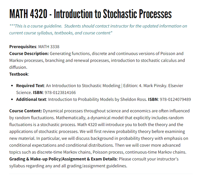
PREREQUISITES 

Course Content: Dynamical processes throughout science and economics are often influenced by random fluctuations. Mathematically, a dynamical model that explicitly includes random fluctuation is a stochastic process. Math 4320 will introduce you to both the theory and the applications of stochastic processes. We will first review probability theory before examining new material. In particular, we will discuss background in probability theory with emphasis on conditional expectations and conditional distributions. Then we will cover more advanced topics such as discrete-time Markov chains, Poisson process, continuous-time Markov chains. Grading \& Make-up Policy/Assignment \& Exam Details: Please consult your instructor’s syllabus regarding any and all grading/assignment guidelines.

MATH4320 Stochastic Process HELP(EXAM HELP, ONLINE TUTOR)

问题 1.

Let $\mathcal{F}$ be a $\sigma$-field on some set $\Omega$.
(1) Show that if $A_1, A_2, \ldots$ are in $\mathcal{F}$, then so is $\cap_{k=1}^{\infty} A_k$.
(2) Show that if $A_1, A_2$ are in $\mathcal{F}$, then so is their symmetric difference $A_1 \triangle A_2:=$ $A_1 \cup A_2-A_1 \cap A_2$.

(1) We prove this by induction. First, note that $A_1\in \mathcal{F}$ by assumption. Now suppose that $\bigcap_{k=1}^n A_k\in\mathcal{F}$ for some $n\geq 1$. Then $A_{n+1}\in\mathcal{F}$ by assumption, so we have $\bigcap_{k=1}^{n+1} A_k = \left(\bigcap_{k=1}^{n} A_k\right) \cap A_{n+1}\in\mathcal{F}$, since $\mathcal{F}$ is a $\sigma$-field and therefore closed under countable intersections.

(2) We have $A_1, A_2\in\mathcal{F}$ by assumption. Since $\mathcal{F}$ is a $\sigma$-field, it is closed under set complements, unions, and intersections. Therefore, we have $A_1^c, A_2^c\in\mathcal{F}$, and hence \begin{align*} A_1\triangle A_2 &= (A_1\cup A_2) \setminus (A_1\cap A_2)\ &= (A_1\cup A_2) \cap (A_1^c \cup A_2^c)\ &= (A_1\cap A_1^c) \cup (A_1\cap A_2^c) \cup (A_2\cap A_1^c) \cup (A_2\cap A_2^c)\ &= (A_1\setminus A_2) \cup (A_2\setminus A_1)\ &= (A_1\cap A_2^c)\cup (A_1^c\cap A_2). \end{align*} Since $\mathcal{F}$ is closed under intersections and unions, we have $A_1\cap A_2^c\in\mathcal{F}$ and $A_1^c\cap A_2\in\mathcal{F}$, and hence $A_1\triangle A_2\in\mathcal{F}$ as desired.

问题 2.

Let $f: U \rightarrow E$ be a function, where $U$ and $E$ are arbitrary sets. For any subset $A \subseteq E$, define
$$
f^{-1}(A)={u \in U ; f(u) \in A}
$$
(i) Show that for all $u \in U$,
$$
1_A(f(u))=1_{f^{-1}(A)}(u)
$$
(ii) Prove that if $\mathcal{E}$ is a $\sigma$-field on $E$, then the collection of subsets of $U$
$$
f^{-1}(\mathcal{E}):=\left{f^{-1}(A) ; A \in \mathcal{E}\right}
$$
is a $\sigma$-field on $U$.

(i) We have $1_A(f(u)) = 1$ if $f(u) \in A$ and $0$ otherwise. On the other hand, $1_{f^{-1}(A)}(u) = 1$ if $u \in f^{-1}(A)$ and $0$ otherwise. But $u \in f^{-1}(A)$ if and only if $f(u) \in A$. Therefore, we have $1_A(f(u)) = 1_{f^{-1}(A)}(u)$ for all $u \in U$.

(ii) We need to show that $f^{-1}(\mathcal{E})$ is a $\sigma$-field on $U$, i.e., it satisfies the following three conditions:

(a) $U \in f^{-1}(\mathcal{E})$; (b) If $A \in f^{-1}(\mathcal{E})$, then $A^c \in f^{-1}(\mathcal{E})$; (c) If $A_1, A_2, \ldots$ are in $f^{-1}(\mathcal{E})$, then $\bigcup_{k=1}^{\infty} A_k \in f^{-1}(\mathcal{E})$.

(a) Since $\mathcal{E}$ is a $\sigma$-field on $E$, we have $E \in \mathcal{E}$, and hence $U = f^{-1}(E) \in f^{-1}(\mathcal{E})$.

(b) Suppose $A \in f^{-1}(\mathcal{E})$. Then $A = f^{-1}(B)$ for some $B \in \mathcal{E}$. Since $\mathcal{E}$ is a $\sigma$-field, we have $B^c \in \mathcal{E}$. Therefore,

A^c = f^{-1}(B^c) = \left(f^{-1}(B)\right)^c \in f^{-1}(\mathcal{E}).Ac=f−1(Bc)=(f−1(B))c∈f−1(E).

(c) Suppose $A_1, A_2, \ldots$ are in $f^{-1}(\mathcal{E})$. Then $A_k = f^{-1}(B_k)$ for some $B_k \in \mathcal{E}$ for each $k$. Since $\mathcal{E}$ is a $\sigma$-field, we have $\bigcup_{k=1}^{\infty} B_k \in \mathcal{E}$. Therefore,

\bigcup_{k=1}^{\infty} A_k = f^{-1}\left(\bigcup_{k=1}^{\infty} B_k\right) \in f^{-1}(\mathcal{E}).k=1⋃∞​Ak​=f−1(k=1⋃∞​Bk​)∈f−1(E).

This completes the proof that $f^{-1}(\mathcal{E})$ is a $\sigma$-field on $U$.

Textbooks


• An Introduction to Stochastic Modeling, Fourth Edition by Pinsky and Karlin (freely
available through the university library here)
• Essentials of Stochastic Processes, Third Edition by Durrett (freely available through
the university library here)
To reiterate, the textbooks are freely available through the university library. Note that
you must be connected to the university Wi-Fi or VPN to access the ebooks from the library
links. Furthermore, the library links take some time to populate, so do not be alarmed if
the webpage looks bare for a few seconds.

此图像的alt属性为空;文件名为%E7%B2%89%E7%AC%94%E5%AD%97%E6%B5%B7%E6%8A%A5-1024x575-10.png
MATH4320 Stochastic Process

Statistics-lab™可以为您提供uh.edu MATH4320 Stochastic Process随机过程课程的代写代考辅导服务! 请认准Statistics-lab™. Statistics-lab™为您的留学生涯保驾护航。

数学代写|MAT270 discrete mathematics

Statistics-lab™可以为您提供tesu.edu MAT270 discrete mathematics离散数学课程的代写代考辅导服务!

数学代写|MAT270 discrete mathematics

MAT270 discrete mathematics课程简介

Discrete Mathematics is designed to meet the needs not only of students majoring in computer science but of a wider audience, especially students in mathematics and science. The course provides tools for formal reasoning. Topics include counting rules, propositional and first-order logic, set theory, functions (with an emphasis on recursive functions), partial order and equivalence relations, Boolean algebra, and switching circuits. Graphs and trees are also introduced. With an emphasis on communication skills, students are required to interpret, describe, discuss, and justify conclusions based on logical reasoning. While the particular focus of the course is on reasoning related to computer programs, no knowledge of programming is required.
Advisory: It is advisable to have knowledge in a course equivalent to MAT-121: College Algebra with a grade of C or better to succeed in this course. Students are responsible for making sure that they have the necessary knowledge.

PREREQUISITES 

Discrete Mathematics is a fundamental course that provides a solid foundation for computer science, mathematics, and science students. The course covers a wide range of topics, including counting rules, logic, set theory, functions, relations, Boolean algebra, and graph theory. The emphasis on formal reasoning and communication skills makes this course valuable to all students.

To succeed in this course, it is advisable to have a good understanding of college algebra, as it forms the basis of many concepts covered in the course. Students should ensure that they have the necessary prerequisite knowledge before enrolling in the course.

The course provides tools for formal reasoning, which are essential for students pursuing computer science or related fields. These tools enable students to analyze and design algorithms, write correct programs, and prove the correctness of programs.

Overall, discrete mathematics is a challenging but rewarding course that prepares students for further study in computer science, mathematics, and science. The skills and knowledge gained in this course are valuable not only in academia but also in industry and other fields.

MAT270 discrete mathematics HELP(EXAM HELP, ONLINE TUTOR)

问题 1.

  1. Let $n \in \mathbb{N}$. Show that the following statements are true
    (1) $n^5 \bmod 5=n \bmod 5$.
    (2) $n^7 \bmod 7=n \bmod 7$.

Proof:

(1) We can use Fermat’s Little Theorem, which states that if $p$ is a prime number and $a$ is an integer not divisible by $p$, then $a^{p-1}\equiv 1 \pmod p$. Applying this theorem with $p=5$ and $a=n$, we have $n^4\equiv 1 \pmod 5$. Multiplying both sides by $n$ gives $n^5 \equiv n \pmod 5$, which is the desired result.

(2) Similarly, we can use Fermat’s Little Theorem with $p=7$ and $a=n$, which gives $n^6\equiv 1 \pmod 7$. Multiplying both sides by $n$ gives $n^7 \equiv n \pmod 7$, which is the desired result.

Therefore, both statements are true.

问题 2.

  1. Prove the following statements. Let $n \in \mathbb{N}, n>1$, and $a \in \mathbb{N}$
    (1) If $a \bmod n=b \bmod n$, then $(-a) \bmod n=(-b) \bmod b$.
    (2) If $p$ is odd prime, then $(-a)^p=-a^p$.

Proof:

(1) Since $a \bmod n=b \bmod n$, we have $n$ divides $a-b$. This means that there exists an integer $k$ such that $a-b=kn$.

Now consider $(-a) \bmod n$ and $(-b) \bmod n$. We want to show that they are equal. We have:

$(-a) \bmod n=(-a+kn-kn) \bmod n=(-a+kn) \bmod n=-(a-kn) \bmod n=-(b-kn) \bmod n=(-b+kn) \bmod n=(-b) \bmod n$

where we have used the fact that adding or subtracting a multiple of $n$ does not change the remainder modulo $n$. Therefore, we have shown that $(-a) \bmod n=(-b) \bmod n$.

(2) We can use the binomial theorem to expand $(-a)^p$:

$(-a)^p=(-1)^p a^p$

If $p$ is odd, then $(-1)^p=-1$, so we have $(-a)^p=-a^p$, which is the desired result.

Therefore, both statements are true.

Textbooks


• An Introduction to Stochastic Modeling, Fourth Edition by Pinsky and Karlin (freely
available through the university library here)
• Essentials of Stochastic Processes, Third Edition by Durrett (freely available through
the university library here)
To reiterate, the textbooks are freely available through the university library. Note that
you must be connected to the university Wi-Fi or VPN to access the ebooks from the library
links. Furthermore, the library links take some time to populate, so do not be alarmed if
the webpage looks bare for a few seconds.


此图像的alt属性为空;文件名为%E7%B2%89%E7%AC%94%E5%AD%97%E6%B5%B7%E6%8A%A5-1024x575-10.png
MAT270 discrete mathematics

Statistics-lab™可以为您提供tesu.edu MAT270 discrete mathematics离散数学课程的代写代考辅导服务! 请认准Statistics-lab™. Statistics-lab™为您的留学生涯保驾护航。

数学代写|信息论作业代写information theory代考|INFM130

如果你也在 怎样代写信息论information theory这个学科遇到相关的难题,请随时右上角联系我们的24/7代写客服。

信息理论是对数字信息的量化、存储和通信的科学研究。该领域从根本上是由哈里-奈奎斯特和拉尔夫-哈特利在20世纪20年代以及克劳德-香农在20世纪40年代的作品所确立的。该领域处于概率论、统计学、计算机科学、统计力学、信息工程和电气工程的交叉点。

statistics-lab™ 为您的留学生涯保驾护航 在代写信息论information theory方面已经树立了自己的口碑, 保证靠谱, 高质且原创的统计Statistics代写服务。我们的专家在代写信息论information theory代写方面经验极为丰富,各种代写信息论information theory相关的作业也就用不着说。

我们提供的信息论information theory及其相关学科的代写,服务范围广, 其中包括但不限于:

  • Statistical Inference 统计推断
  • Statistical Computing 统计计算
  • Advanced Probability Theory 高等概率论
  • Advanced Mathematical Statistics 高等数理统计学
  • (Generalized) Linear Models 广义线性模型
  • Statistical Machine Learning 统计机器学习
  • Longitudinal Data Analysis 纵向数据分析
  • Foundations of Data Science 数据科学基础

数学代写|信息论作业代写information theory代考|Bounded linear operators

Let $\mathrm{X}$ and $\mathrm{Y}$ be complex Banach spaces (or Hilbert spaces) equipped with the norm $|\cdot|_{\mathrm{X}}$ and $|\cdot|_{\mathrm{Y}}$, respectively.

A linear map $\mathbf{T}: \operatorname{dom}(\mathbf{T}) \subset X \rightarrow \mathbb{Y}$ is said to be a bounded linear map if $\mathbf{T}(B)$ is a bounded subset of $Y$ for every bounded $B \subset \operatorname{dom}(\mathbf{T}) \subset X$. Equivalently, $T$ is a bounded linear map if there exists a constant $K>0$ (that depends on $\mathrm{T}$ only) such that
$$
|\mathrm{T} \psi|_{\mathrm{Y}} \leq K|\psi|_{\mathrm{X}}, \quad \forall \psi \in \operatorname{dom}(\mathrm{T}) \subset \mathrm{X}
$$

In this case, it can be proved (see, e. g., Reed and Simon [128] and Rudin [134]) that $\operatorname{dom}(\mathbf{T})=\mathbf{X}$. The collection of bounded linear maps from $\mathbb{X}$ to $\mathbb{Y}$ will be denoted by $\mathfrak{B}(\mathbb{X}, \mathbf{Y})$. If $\mathbb{X}=\mathbb{Y}$, then $\mathfrak{B}(\mathbb{X}, \mathbf{Y})$ can be written as $\mathfrak{B}(\mathbb{X})$ and $\mathbf{T} \in \mathfrak{B}(\mathbb{X})$ will be called a bounded linear operator.

The following is a Banach-Schauder theorem, which is also known as an open mapping theorem. A proof can be found in standard functional analysis texts such as Rudin [133] and is omitted here.

Theorem 1.2.1 (Banach-Schauder theorem). If $\mathrm{X}$ and $\mathrm{Y}$ are complex Banach spaces or complex Hilbert spaces and $\mathbf{T}: \mathbb{X} \rightarrow \mathbb{Y}$ is a surjective (or onto) bounded linear operator, then $\mathbf{T}$ is an open map (i.e., if $U$ is an open set in $\mathbf{X}$, then $\mathbf{T}(U)$ is open in $\mathbb{Y}$ ).
We have the following corollary.
Corollary 1.2.2. If $\mathrm{X}$ and $\mathrm{Y}$ are complex Banach or Hilbert spaces and $\mathbf{T} \in \mathcal{L}(\mathbb{X}, \mathbb{Y})$ is invertible (i.e., a bijective linear map), then the inverse map, $\mathbf{T}^{-1}$, is bounded, i. e., $\mathbf{T}^{-1} \in \mathfrak{B}(\mathbf{Y}, \mathbf{X})$. (Note that $\mathbf{T}^{-1}$ is automatically linear.)
If $\mathbf{T} \in \mathfrak{B}(\mathbb{X})$, we define the operator norm $|\mathbf{T}|_{\infty}$ of $\mathbf{T}$ as
$$
|\mathbf{T}|_{\infty}=\sup {\phi \neq 0} \frac{|\mathbf{T} \phi|{\mathrm{X}}}{|\phi|_{\mathrm{X}}}=\sup {|\phi|{\mathrm{X}}=1}|\mathbf{T} \phi|_{\mathrm{X}}
$$
There are two trivial bounded linear operators $\mathbf{0}{\mathbf{X}}$ (the zero operator) and $\mathbf{I}{\mathbf{X}}$ (the identity operator) that will appear often throughout the book. The zero operator $\mathbf{0}{\mathrm{X}}$ is the operator that maps every vector $\phi \in \mathbb{X}$ to the zero vector $\mathbf{0}$ in X (i. e., $\mathbf{0}{\mathrm{X}} \phi=\mathbf{0}$ for all $\phi \in \mathbb{X})$ and the identity operator $\mathbf{I}{\mathrm{H}}$ is the operator that maps every vector $\phi \in \mathbb{X}$ to itself (i. e., $\mathbf{I}{\mathbf{X}} \phi=\phi$ for all $\phi \in \mathrm{X}$.)

数学代写|信息论作业代写information theory代考|Positive operators

A linear (but not necessary bounded) operator $\mathbf{T} \in \mathfrak{L}(\mathbb{H})$ on a complex Hilbert space $\mathbb{H}$ is said to be positive and to be denoted by $\mathbf{T} \geq \mathbf{0}$ if $\langle\mathbf{T} \varphi, \varphi\rangle_{\mathbf{H}} \geq 0$ for all $\varphi \in \operatorname{dom}(\mathbf{T})$.

Let $\mathbf{T}_1, \mathbf{T}_2 \in \mathfrak{L}(\mathbb{H})$. We say that $\mathbf{T}_1 \geq \mathbf{T}_2$ if $\mathbf{T}_1-\mathbf{T}_2:=\mathbf{T}_1+\left(-\mathbf{T}_2\right) \geq \mathbf{0}$, where $-\mathbf{T}$ is the linear operator such that $\mathbf{T}+(-\mathbf{T})=\mathbf{0}$.

The set of all positive linear operators (resp., positive bounded linear operators) on $\mathbb{H}$ will be denoted by $\mathfrak{L}{+}(\mathbb{H})$ (resp., $\mathfrak{B}{+}(\mathbb{H})$ ). Both $\mathfrak{L}{+}(\mathbb{H})$ and $\mathfrak{B}{+}(\mathbb{H})$ are positive cones in the sense that $\mathbf{T} \in \mathfrak{L}{+}(\mathbb{H})$ (resp., $\mathfrak{B}{+}(\mathbb{H})$ ) and $c>0$ imply that $c \mathbf{T} \in \mathfrak{L}{+}(\mathbb{H})$ (resp., $\left.\mathfrak{B}{+}(\mathbb{H})\right)$

A sequence of bounded linear operators $\left(\mathbf{A}n\right){n=1}^{+\infty} \subset \mathfrak{B}(\mathbb{H})$ is said to converge strongly to $\mathbf{A} \in \mathfrak{B}(\mathbb{H})$ if
$$
\lim {n \rightarrow+\infty}\left|\mathbf{A}_n \phi-\mathbf{A} \phi\right|{\mathrm{H}}=0, \quad \forall \phi \in \mathbb{H}
$$
We will use the following monotone convergence theorem of a sequence of nondecreasing positive bounded linear operators.

Theorem 1.3.1 (Monotone convergence theorem for operators). Let $\quad\left(\mathbf{A}n\right){n=1}^{+\infty}$ be $a$ bounded monotone sequence of bounded linear operators on $\mathbb{H}$. Then the sequence $\left(\mathbf{A}n\right){n=1}^{+\infty}$ is strongly convergent.
Proof. Assume, for example, that $\left(\mathbf{A}n\right){n=1}^{+\infty}$ is such that
$$
\mathbf{A}1 \leq \mathbf{A}_2 \leq \cdots \leq \mathbf{A}_n \leq \cdots \leq \mathbf{M} $$ for some $\mathbf{M} \in \mathfrak{B}(\mathbb{H})$. Since $\sup _n\left|\mathbf{A}_n\right|{\infty} \leq|\mathbf{M}|_{\infty}<+\infty$, we obtain that for any $\phi \in \mathbb{H}$ the sequence $\left\langle\mathbf{A}n \phi, \phi\right\rangle{\mathbb{H}}$ is convergent. Therefore, due to “polarization” (1.13),
$$
\begin{aligned}
\left\langle\mathbf{A}n \phi, \psi\right\rangle & =\frac{1}{4}\left{\left\langle\mathbf{A}_n(\phi+\psi), \phi+\psi\right\rangle{\mathbb{H}}-\left\langle\mathbf{A}n(\phi-\psi), \phi-\psi\right\rangle{\mathbb{H}}\right. \
& \left.+\iota\left[\left\langle\mathbf{A}n(\phi+\imath \psi), \phi+\imath \psi\right\rangle{\mathbb{H}}-\left\langle\mathbf{A}n(\phi-\imath \psi), \phi-\imath \psi\right\rangle{\mathbf{H}}\right]\right} .
\end{aligned}
$$

信息论代写

数学代写|信息论作业代写information theory代考|Bounded linear operators

让 $X$ 和 $Y$ 是配备规范的复杂 Banach 空间 (或 Hilbert 空间) $|\cdot|{ }X$ 和 $|\cdot|_Y$ ,分别。 线性映射 $\mathbf{T}: \operatorname{dom}(\mathbf{T}) \subset X \rightarrow \mathbb{Y}$ 被称为有界线性映射如果 $\mathbf{T}(B)$ 是的有界子集 $Y$ 对于每一个有界 $B \subset \operatorname{dom}(\mathbf{T}) \subset X$. 等价地, $T$ 是有界线性映射,如果存在常数 $K>0$ (这取决于 $\mathrm{T}$ 仅) 这样 $$ |\mathrm{T} \psi|{\mathrm{Y}} \leq K|\psi|{\mathrm{X}}, \quad \forall \psi \in \operatorname{dom}(\mathrm{T}) \subset \mathrm{X} $$ 在这种情况下,可以证明(参见 Reed 和 Simon [128] 以及 Rudin [134]) $\operatorname{dom}(\mathbf{T})=\mathbf{X}$. 有界线性映射 的集合来自 $\mathbb{X}$ 到 $\mathbb{Y}$ 将被表示为 $\mathfrak{B}(\mathbb{X}, \mathbf{Y})$. 如果 $\mathbb{X}=\mathbb{Y}$ ,然后 $\mathfrak{B}(\mathbb{X}, \mathbf{Y})$ 可以写成 $\mathfrak{B}(\mathbb{X})$ 和 $\mathbf{T} \in \mathfrak{B}(\mathbb{X})$ 将 被称为有界线性算子。 以下是 Banach-Schauder 定理,也称为开映射定理。可以在 Rudin [133] 等标准功能分析文本中找到证 明,此处省略。 定理 1.2.1 (Banach-Schauder 定理) 。如果X和 $Y$ 是复 Banach 空间或复 Hilbert 空间和 $\mathbf{T}: \mathbb{X} \rightarrow \mathbb{Y}$ 是 满射 (或满射) 有界线性算子,则 $\mathbf{T}$ 是一个开放映射 (即,如果 $U$ 是一个开集 $\mathbf{X}$ ,然后 $\mathbf{T}(U)$ 打开于 $\mathbb{Y}$ ). 我们有以下推论。 推论 1.2.2。如果 $X$ 和 $Y$ 是复 Banach 或 Hilbert 空间和 $\mathbf{T} \in \mathcal{L}(\mathbb{X}, \mathbb{Y})$ 是可逆的(即双射线生映射),那 么逆映射, $\mathbf{T}^{-1}$ ,是有界的,即 $\mathbf{T}^{-1} \in \mathfrak{B}(\mathbf{Y}, \mathbf{X})$. (注意 $\mathbf{T}^{-1}$ 是自动线性的。) 如果 $\mathbf{T} \in \mathfrak{B}(\mathbb{X})$ ,我们定义算子范数 $|\mathbf{T}|{\infty}$ 的 $\mathbf{T}$ 作为
$$
|\mathbf{T}|{\infty}=\sup \phi \neq 0 \frac{|\mathbf{T} \phi| \mathrm{X}}{|\phi|{\mathrm{X}}}=\sup |\phi| \mathrm{X}=1|\mathbf{T} \phi|_{\mathrm{X}}
$$
有两个平凡的有界线生算子 $\mathbf{0 X}$ (零运算符) 和IX (身份运算符) 将在整本书中经常出现。零运算符 $\mathbf{O X}$ 是映射每个向量的运算符 $\phi \in \mathbb{X}$ 到零向量 0 在 X (即 $0 \mathrm{X} \phi=\mathbf{0}$ 对全部 $\phi \in \mathbb{X}$ )和身份运营商IH是映射每 个向量的运算符 $\phi \in \mathbb{X}$ 对自己 (即IXX $\phi=\phi$ 对全部 $\phi \in \mathbf{X}$.)

数学代写|信息论作业代写information theory代考|Positive operators

线性 (但不一定有界) 运算符 $\mathbf{T} \in \mathfrak{L}(\mathbb{H})$ 在复杂的 Hilbert 空间上 $\mathbb{H}$ 据说是积极的,并表示为 $\mathbf{T} \geq \mathbf{0}$ 如 果 $\langle\mathbf{T} \varphi, \varphi\rangle_{\mathbf{H}} \geq 0$ 对全部 $\varphi \in \operatorname{dom}(\mathbf{T})$.
让 $\mathbf{T}1, \mathbf{T}_2 \in \mathfrak{L}(\mathbb{H})$. 我们说 $\mathbf{T}_1 \geq \mathbf{T}_2$ 如果 $\mathbf{T}_1-\mathbf{T}_2:=\mathbf{T}_1+\left(-\mathbf{T}_2\right) \geq \mathbf{0}$ , 在哪里 $-\mathbf{T}$ 是这样的线 性算子 $\mathbf{T}+(-\mathbf{T})=\mathbf{0}$ 上所有正线性算子 (分别为正有界线性算子) 的集合茑将被表示为 $\mathfrak{L}+(\mathbb{H})$ (分别, $\mathfrak{B}+(\mathbb{H})$ ). 两个都 $\mathfrak{L}+(\mathbb{H})$ 和 $\mathfrak{B}+(\mathbb{H})$ 在某种意义上是正锥 $\mathbf{T} \in \mathfrak{L}+(\mathbb{H})$ (分别, $\mathfrak{B}+(\mathbb{H})$ ) 和 $c>0$ 暗示 $c \mathbf{T} \in \mathfrak{L}+(\mathbb{H})$ $($ 分别, $\mathfrak{B}+(\mathbb{H}))$ 有界线性算子序列 $(\mathbf{A} n) n=1^{+\infty} \subset \mathfrak{B}(\mathbb{H})$ 据说强烈收敛到 $\mathbf{A} \in \mathfrak{B}(\mathbb{H})$ 如果 $$ \lim n \rightarrow+\infty\left|\mathbf{A}_n \phi-\mathbf{A} \phi\right| \mathrm{H}=0, \quad \forall \phi \in \mathbb{H} $$ 我们将使用以下一系列非递减正有界线性算子的单调收敛定理。 定理 1.3.1 (算子的单调收敛定理) 。让 $(\mathbf{A} n) n=1^{+\infty}$ 是 $a$ 有界线性算子的有界单调序列 $\mathbb{H}$. 然后顺 序 $(\mathbf{A} n) n=1^{+\infty}$ 是强收敛的。 证明。例如,假设 $(\mathbf{A} n) n=1^{+\infty}$ 是这样的 $$ \mathbf{A} 1 \leq \mathbf{A}_2 \leq \cdots \leq \mathbf{A}_n \leq \cdots \leq \mathbf{M} $$ 对于一些 $\mathbf{M} \in \mathfrak{B}(\mathbb{H})$. 自从 $\sup _n\left|\mathbf{A}_n\right| \infty \leq|\mathbf{M}|{\infty}<+\infty$ ,我们得到任何 $\phi \in \mathbb{H}$ 序列 $\langle\mathbf{A} n \phi, \phi\rangle \mathbb{H}$ 是收敛的。因此,由于”极化” (1.13),

数学代写|信息论作业代写information theory代考 请认准statistics-lab™

统计代写请认准statistics-lab™. statistics-lab™为您的留学生涯保驾护航。

金融工程代写

金融工程是使用数学技术来解决金融问题。金融工程使用计算机科学、统计学、经济学和应用数学领域的工具和知识来解决当前的金融问题,以及设计新的和创新的金融产品。

非参数统计代写

非参数统计指的是一种统计方法,其中不假设数据来自于由少数参数决定的规定模型;这种模型的例子包括正态分布模型和线性回归模型。

广义线性模型代考

广义线性模型(GLM)归属统计学领域,是一种应用灵活的线性回归模型。该模型允许因变量的偏差分布有除了正态分布之外的其它分布。

术语 广义线性模型(GLM)通常是指给定连续和/或分类预测因素的连续响应变量的常规线性回归模型。它包括多元线性回归,以及方差分析和方差分析(仅含固定效应)。

有限元方法代写

有限元方法(FEM)是一种流行的方法,用于数值解决工程和数学建模中出现的微分方程。典型的问题领域包括结构分析、传热、流体流动、质量运输和电磁势等传统领域。

有限元是一种通用的数值方法,用于解决两个或三个空间变量的偏微分方程(即一些边界值问题)。为了解决一个问题,有限元将一个大系统细分为更小、更简单的部分,称为有限元。这是通过在空间维度上的特定空间离散化来实现的,它是通过构建对象的网格来实现的:用于求解的数值域,它有有限数量的点。边界值问题的有限元方法表述最终导致一个代数方程组。该方法在域上对未知函数进行逼近。[1] 然后将模拟这些有限元的简单方程组合成一个更大的方程系统,以模拟整个问题。然后,有限元通过变化微积分使相关的误差函数最小化来逼近一个解决方案。

tatistics-lab作为专业的留学生服务机构,多年来已为美国、英国、加拿大、澳洲等留学热门地的学生提供专业的学术服务,包括但不限于Essay代写,Assignment代写,Dissertation代写,Report代写,小组作业代写,Proposal代写,Paper代写,Presentation代写,计算机作业代写,论文修改和润色,网课代做,exam代考等等。写作范围涵盖高中,本科,研究生等海外留学全阶段,辐射金融,经济学,会计学,审计学,管理学等全球99%专业科目。写作团队既有专业英语母语作者,也有海外名校硕博留学生,每位写作老师都拥有过硬的语言能力,专业的学科背景和学术写作经验。我们承诺100%原创,100%专业,100%准时,100%满意。

随机分析代写


随机微积分是数学的一个分支,对随机过程进行操作。它允许为随机过程的积分定义一个关于随机过程的一致的积分理论。这个领域是由日本数学家伊藤清在第二次世界大战期间创建并开始的。

时间序列分析代写

随机过程,是依赖于参数的一组随机变量的全体,参数通常是时间。 随机变量是随机现象的数量表现,其时间序列是一组按照时间发生先后顺序进行排列的数据点序列。通常一组时间序列的时间间隔为一恒定值(如1秒,5分钟,12小时,7天,1年),因此时间序列可以作为离散时间数据进行分析处理。研究时间序列数据的意义在于现实中,往往需要研究某个事物其随时间发展变化的规律。这就需要通过研究该事物过去发展的历史记录,以得到其自身发展的规律。

回归分析代写

多元回归分析渐进(Multiple Regression Analysis Asymptotics)属于计量经济学领域,主要是一种数学上的统计分析方法,可以分析复杂情况下各影响因素的数学关系,在自然科学、社会和经济学等多个领域内应用广泛。

MATLAB代写

MATLAB 是一种用于技术计算的高性能语言。它将计算、可视化和编程集成在一个易于使用的环境中,其中问题和解决方案以熟悉的数学符号表示。典型用途包括:数学和计算算法开发建模、仿真和原型制作数据分析、探索和可视化科学和工程图形应用程序开发,包括图形用户界面构建MATLAB 是一个交互式系统,其基本数据元素是一个不需要维度的数组。这使您可以解决许多技术计算问题,尤其是那些具有矩阵和向量公式的问题,而只需用 C 或 Fortran 等标量非交互式语言编写程序所需的时间的一小部分。MATLAB 名称代表矩阵实验室。MATLAB 最初的编写目的是提供对由 LINPACK 和 EISPACK 项目开发的矩阵软件的轻松访问,这两个项目共同代表了矩阵计算软件的最新技术。MATLAB 经过多年的发展,得到了许多用户的投入。在大学环境中,它是数学、工程和科学入门和高级课程的标准教学工具。在工业领域,MATLAB 是高效研究、开发和分析的首选工具。MATLAB 具有一系列称为工具箱的特定于应用程序的解决方案。对于大多数 MATLAB 用户来说非常重要,工具箱允许您学习应用专业技术。工具箱是 MATLAB 函数(M 文件)的综合集合,可扩展 MATLAB 环境以解决特定类别的问题。可用工具箱的领域包括信号处理、控制系统、神经网络、模糊逻辑、小波、仿真等。

R语言代写问卷设计与分析代写
PYTHON代写回归分析与线性模型代写
MATLAB代写方差分析与试验设计代写
STATA代写机器学习/统计学习代写
SPSS代写计量经济学代写
EVIEWS代写时间序列分析代写
EXCEL代写深度学习代写
SQL代写各种数据建模与可视化代写

数学代写|信息论作业代写information theory代考|CSYS5030

如果你也在 怎样代写信息论information theory这个学科遇到相关的难题,请随时右上角联系我们的24/7代写客服。

信息理论是对数字信息的量化、存储和通信的科学研究。该领域从根本上是由哈里-奈奎斯特和拉尔夫-哈特利在20世纪20年代以及克劳德-香农在20世纪40年代的作品所确立的。该领域处于概率论、统计学、计算机科学、统计力学、信息工程和电气工程的交叉点。

statistics-lab™ 为您的留学生涯保驾护航 在代写信息论information theory方面已经树立了自己的口碑, 保证靠谱, 高质且原创的统计Statistics代写服务。我们的专家在代写信息论information theory代写方面经验极为丰富,各种代写信息论information theory相关的作业也就用不着说。

我们提供的信息论information theory及其相关学科的代写,服务范围广, 其中包括但不限于:

  • Statistical Inference 统计推断
  • Statistical Computing 统计计算
  • Advanced Probability Theory 高等概率论
  • Advanced Mathematical Statistics 高等数理统计学
  • (Generalized) Linear Models 广义线性模型
  • Statistical Machine Learning 统计机器学习
  • Longitudinal Data Analysis 纵向数据分析
  • Foundations of Data Science 数据科学基础

数学代写|信息论作业代写information theory代考|Complex Hilbert and Banach spaces

This section serves as a review of complex Hilbert and Banach spaces. Some of the frequently used theorems and/or propositions are stated without a proof.

Complex Hilbert spaces play an important role in the description of quantum systems. As mentioned in Chang [24], every quantum system is associated with an infinite-dimensional separable or a finite-dimensional complex Hilbert space, which consists of the states of the quantum system. In physics terminology, the Hilbert space is usually referred to as the space of (pure) states. Throughout this monograph, the mathematical description of a quantum system shall be based on a certain complex (separable) Hilbert space $\mathbb{H}$ and, therefore, the quantum system will simply be denoted by $\mathbb{H}$.

The quantum system $\mathbb{H}$ is said to be a finite-dimensional system if $\mathbb{H}$ is a finitedimensional complex Hilbert space. Otherwise, the quantum system $\mathbb{H}$ is said to be an infinite-dimensional system.
We first set some basic notation below.
Let $\mathbb{R}$ and $\mathbb{C}$ denote the field of real numbers and the field of complex numbers, respectively. If $z=x+i y \in \mathbb{C}$, where $x, y \in \mathbb{R}$, let $\bar{z}=x-i y \in \mathbb{C}$ and $|z|=\sqrt{x^2+y^2} \in$ $\mathbb{R}_{+}$denote the complex conjugate and the modulus of the complex number $z \in \mathbb{C}$, respectively. In this case, $x=\mathbb{R}(z)$ is the real part of $z$ and $y=J(z)$ is the imaginary part of $z$. Throughout the end, elements in $\mathbb{R}$ or $\mathbb{C}$ shall be denoted by lowercase letters such as $a, b$ or $c$ and sometimes lower case Greek alphabets such as $\lambda$ and $\alpha$.
We also use the following conventional notation throughout the book:

  • $\quad \mathbb{N}$ is the set of all natural numbers, positive integers, i. e., $\mathbb{N}={1,2, \cdots, n, \cdots}$.
  • $\mathbb{Z}$ is the set of all integers, i. e., $\mathbb{Z}={\cdots,-2,-1,0,1,2, \cdots}$.
  • $\mathbb{Z}{+}$is the set of nonnegative integers, i. e., $\mathbb{Z}{+}=\mathbb{N} \cup{0}$.
    $-\mathbb{R}_{+}={c \in \mathbb{R} \mid c \geq 0}$.
  • For – $\infty a<b<+\infty$, we use the usual convention for closed, open and halfopen intervals on the real line $\mathbb{R}$ such as $[a, b],[a, b[] a, b],]-\infty, a],]-\infty, a[$, $[b,+\infty[$ and $] b, \infty[$, etc.

Let $\mathbb{H}$ be a (generic) Hilbert space over the field of complex numbers $\mathbb{C}$ and be referred to as a complex Hilbert space throughout the end.

数学代写|信息论作业代写information theory代考|Linear operators and their adjoints

Let $\mathrm{X}$ and $\mathrm{Y}$ be two separable complex Banach spaces equipped with Banach norms $|\cdot|_{\mathrm{X}}$ and $|\cdot|_{\mathrm{Y}}$, respectively.
A map (or transformation) $\mathbf{T}: \operatorname{dom}(\mathbf{T}) \subseteq \mathbb{X} \rightarrow \mathbb{Y}$ is said to be linear if
$$
a \phi+b \psi \in \operatorname{dom}(\mathbf{T})
$$
and
$$
\mathbf{T}(a \phi+b \psi)=a \mathbf{T}(\phi)+b \mathbf{T}(\psi), \quad \forall a, b \in \mathbb{C} \text { and } \forall \phi, \psi \in \operatorname{dom}(\mathbf{T})
$$
where $\operatorname{dom}(\mathbf{T}) \subseteq \mathbf{X}$ is called the domain of $\mathbf{T}$. Note that dom $(\mathbf{T}) \neq \mathbf{X}$, in general. However, it is known that dom(T) is a dense subset of $X$.
The following are some known cases where $\operatorname{dom}(T)=X$ :
(i) $\mathbf{T}$ is a bounded linear operator (see the following subsection for the definition of a bounded linear operator);
(ii) $\mathbb{X}=\mathbb{H}$ is a Hilbert space and $\operatorname{dim}(\mathbb{H})<+\infty$, where $\operatorname{dim}(\mathbb{H})$ denotes the dimension of $\mathbb{H}$. In this case, every linear operator is a bounded linear operator (see (1.10) below for the definition of a bounded linear operator).

Assuming dom $(T)$ is dense in $\mathrm{X}$ or $\operatorname{dom}(T)=X$, the collection of such linear maps will be denoted by $\mathfrak{L}(X, \mathbb{Y})$. The linear map T will be called a linear operator if $\operatorname{dom}(\mathbf{T}) \subseteq$ $X=\mathbb{Y}$. The collection of linear operators will be denoted by $\mathcal{L}(X)$.

Throughout to the end, linear maps/operators on a complex Banach or Hilbert space will be denoted by boldfaced letters such as $\mathbf{S}, \mathbf{T}, \mathbf{a}, \mathbf{b}, \mathbf{X}, \mathbf{Y}$, etc., and a linear $\operatorname{map} T \in \mathfrak{L}(\mathbb{X}, \mathrm{Y})$ acting on a vector $\phi \in \mathbb{X}$ will be denoted by either $\mathbf{T} \phi$ or $\mathbf{T}(\phi)$.

Let $\mathbf{T}: \operatorname{dom}(\mathbf{T}) \rightarrow \operatorname{range}(\mathbf{T})$ (where $\operatorname{range}(\mathbf{T}):={\mathbf{T} \phi \in \mathbb{Y} \mid \phi \in \operatorname{dom}(\mathbf{T}) \subset \mathbf{X}}$ denotes the range of $\mathbf{T}$ ) be a bijective (one-to-one and onto) linear map. A linear map $\mathbf{S}:$ range(T) $\rightarrow \operatorname{dom}(\mathbf{S})$ is said to be the inverse of $\mathbf{T}$ if $\mathbf{S} \circ \mathbf{T}=\mathbf{I}{\mathbf{X}}$ and $\mathbf{T} \circ \mathbf{S}=\mathbf{I}{\mathbb{Y}}$, where $\mathbf{I}{\mathrm{X}}$ and $\mathbb{I}{\mathrm{Y}}$ are the identity operator on $\mathrm{X}$ and $\mathbb{Y}$, respectively. That is, $\mathbf{I}{\mathbf{X}}(x)=x$ for all $x \in \mathbb{X}$ and $\mathbf{I}{\mathrm{Y}}(y)=y$ for all $y \in \mathbb{Y}$. In this case, we write $\mathbf{S}=\mathbf{T}^{-1}$.

For a linear map $\mathbf{T}: \operatorname{dom}(\mathbf{T}) \subset \mathbb{H} \rightarrow \mathbb{K}$, where $\mathbb{H}$ and $\mathbb{K}$ are complex Hilbert spaces, $\operatorname{ker}(\mathbf{T})$ (the kernel of $\mathbf{T}$ ), range(T) (the range of $\mathbf{T}$ ) and $\operatorname{supp}(\mathbf{T}$ ) (the support of T) are defined as:
$$
\begin{aligned}
\operatorname{ker}(\mathbf{T}) & ={\phi \in \operatorname{dom}(\mathbf{T}) \subset \mathbb{H} \mid \mathbf{T} \phi=0} \
\operatorname{range}(\mathbf{T}) & ={\psi \in \mathbb{K} \mid \psi=\mathbf{T} \phi \text { for some } \phi \in \operatorname{dom}(\mathbf{T}) \subset \mathbb{H}} \
\operatorname{supp}(\mathbf{T}) & =(\operatorname{ker}(\mathbf{T}))^{\perp}:=\left{\psi \in \mathbb{H} \mid\langle\psi, \phi\rangle_{\mathbf{H}}=0, \forall \phi \in \operatorname{ker}(\mathbf{T})\right}
\end{aligned}
$$
A linear map $\mathbf{T}: \operatorname{dom}(\mathbf{T}) \rightarrow \mathbb{K}$ is said to be closed if its graph,
$$
\operatorname{graph}(\mathbf{T}):={(\phi, \mathbf{T}(\phi)) \in \mathbb{H} \times \mathbb{K} \mid \phi \in \operatorname{dom}(\mathbf{T})}
$$
is a closed subset of $\mathbb{H} \times \mathbb{K}$.

信息论代写

数学代写|信息论作业代写information theory代考|Complex Hilbert and Banach spaces

本节回顾复数 Hilbert 和 Banach 空间。一些常用的定理和/或命题在没有证明的情况下陈述。
复 Hilbert 空间在描述量子系统中起着重要作用。正如 Chang [24] 中提到的,每个量子系统都与一个无限 维可分离或有限维复 Hilbert 空间相关联,该空间由量子系统的状态组成。在物理学术语中,希尔伯特空 间通常被称为 (纯) 态空间。在本专着中,量子系统的数学描述应基于某个复杂的 (可分离的) 布尔伯特 空间 $\mathbb{H}$ 因此,量子系统将简单地表示为 $\mathbb{H}$.
量子系统 $\mathbb{H}$ 被称为有限维系统,如果 $\mathbb{H}$ 是一个有限维复 Hilbert 空间。否则,量子系统田被称为无限维系 统。
我们首先在下面设置一些基本符号。
让 $\mathbb{R}$ 和 $\mathbb{C}$ 分别表示实数域和复数域。如果 $z=x+i y \in \mathbb{C}$ ,在哪里 $x, y \in \mathbb{R}$ ,让 $\bar{z}=x-i y \in \mathbb{C}$ 和 $|z|=\sqrt{x^2+y^2} \in \mathbb{R}_{+}$表示复共轭和复数的模 $z \in \mathbb{C}$ ,分别。在伩种情况下, $x=\mathbb{R}(z)$ 是的真实部 分 $z$ 和 $y=J(z)$ 是的虚部 $z$. 在整个结尾,元素在 $\mathbb{R}$ 或者 $\mathbb{C}$ 应由小写字母表示,例如 $a, b$ 或者 $c$ 有时是小写 晞腊字母,例如 $\lambda$ 和 $\alpha$.
我们还在整本书中使用以下常规符号:

  • $\mathbb{N}$ 是所有自然数、正整数的集合,即 $\mathbb{N}=1,2, \cdots, n, \cdots$.
  • $\mathbb{Z}$ 是所有整数的集合,即 $\mathbb{Z}=\cdots,-2,-1,0,1,2, \cdots$.
  • $\mathbb{Z}+$ 是非负整数的集合,即 $\mathbb{Z}+=\mathbb{N} \cup 0$.
    $-\mathbb{R}_{+}=c \in \mathbb{R} \mid c \geq 0$.
  • 为了- $\infty a<b<+\infty$ ,我们对实线上的闭区间、开区间和半开区间使用通常的约定 $\mathbb{R}$ 例如 $[a, b],[a, b[] a, b],]-\infty, a],]-\infty, a[,[b,+\infty[$ 和 $] b, \infty[$, ETC。
    让 $\mathbb{H}$ 是复数域上的 (通用) 桸尔伯特空间 $\mathbb{C}$ 并始终被称为复杂的希尔伯特空间。

数学代写|信息论作业代写information theory代考|Linear operators and their adjoints

让 $\mathrm{X}$ 和 $Y$ 是配备 Banach 范数的两个可分离的复杂 Banach 空间 $|\cdot|{ }_X$ 和 $|\cdot|_Y$ ,分别。 映射 (或转换) $\mathbf{T}: \operatorname{dom}(\mathbf{T}) \subseteq \mathbb{X} \rightarrow \mathbb{Y}$ 据说是线性的,如果
$$
a \phi+b \psi \in \operatorname{dom}(\mathbf{T})
$$

$$
\mathbf{T}(a \phi+b \psi)=a \mathbf{T}(\phi)+b \mathbf{T}(\psi), \quad \forall a, b \in \mathbb{C} \text { and } \forall \phi, \psi \in \operatorname{dom}(\mathbf{T})
$$
在哪里 $\operatorname{dom}(\mathbf{T}) \subseteq \mathbf{X}$ 被称为域 $\mathbf{T}$. 请注意, $\operatorname{dom}(\mathbf{T}) \neq \mathbf{X} , 一$ 般来说。然而,众所周知, $\operatorname{dom}(\mathrm{T})$ 是 $X$
以下是一些已知案例,其中 $\operatorname{dom}(T)=X: \quad($
一) $\mathbf{T}$ 是有界线性算子 (有关有界线性算子的定义,请参见以下小节);
$($ 二) $\mathbb{X}=\mathbb{H}$ 是㹷尔伯特空间并且 $\operatorname{dim}(\mathbb{H})<+\infty$ ,在哪里 $\operatorname{dim}(\mathbb{H})$ 表示维度 $\mathbb{H}$. 在这种情况下,每个线 性算子都是有界线性算子(有关有界线性算子的定义,请参见下面的 (1.10))。
假设 $\operatorname{dom}(T)$ 密集在 $\mathrm{X}$ 或者 $\operatorname{dom}(T)=X$ ,此类线性映射的集合将表示为 $\mathfrak{L}(X, \mathbb{Y})$. 线性映射 $\mathrm{T}$ 将被称 为线性算子,如果 $\operatorname{dom}(\mathbf{T}) \subseteq X=\mathbb{Y}$. 线性算子的集合将表示为 $\mathcal{L}(X)$.
从始至终,复杂 Banach 或 Hilbert 空间上的线性映射/算子将用粗体字母表示,例如 $\mathbf{S}, \mathbf{T}, \mathbf{a}, \mathbf{b}, \mathbf{X}, \mathbf{Y}$ 等,以及一个线性 $\operatorname{map} T \in \mathfrak{L}(\mathbb{X}, \mathrm{Y})$ 作用于向量 $\phi \in \mathbb{X}$ 将被表示为 $\mathbf{T} \phi$ 或者 $\mathbf{T}(\phi)$.
让 $\mathbf{T}: \operatorname{dom}(\mathbf{T}) \rightarrow \operatorname{range}(\mathbf{T})$ (在哪里range $(\mathbf{T}):=\mathbf{T} \phi \in \mathbb{Y} \mid \phi \in \operatorname{dom}(\mathbf{T}) \subset \mathbf{X}$ 表示范围 $\mathbf{T})$ 是 一个双射 (一对一和到) 线性映射。线性映射 $\mathbf{S}:$ :量程 $(T) \rightarrow \operatorname{dom}(\mathbf{S})$ 据说是的倒数 $\mathbf{T}$ 如果 $\mathbf{S} \circ \mathbf{T}=\mathbf{I X}$ 和 $\mathbf{T} \circ \mathbf{S}=\mathbf{I} Y$ , 在哪里 $\mathbf{I X}$ 和 IY 身份运算符在 $\mathrm{X}$ 和 $\mathbb{Y}$ ,分别。那是, $\mathbf{I X}(x)=x$ 对全部 $x \in \mathbb{X}$ 和 $\mathbf{I Y}(y)=y$ 对全部 $y \in \mathbb{Y}$. 在这种情况下,我们写 $\mathbf{S}=\mathbf{T}^{-1}$.
对于线性映射 $\mathbf{T}: \operatorname{dom}(\mathbf{T}) \subset \mathbb{H} \rightarrow \mathbb{K}$ , 在哪里 $\mathbb{H}$ 和 $\mathbb{K}$ 是复莃尔伯特空间, $\operatorname{ker}(\mathbf{T})$ (内核的 $\mathbf{T})$, 范围 (T) (范围 $\mathbf{T})$ 和 $\operatorname{supp}(\mathbf{T})$ ( $\mathrm{T}$ 的支持) 定义为:
\begin } { \text { aligned } } \text { loperatorname{ker } } ( \backslash m a t h b f { T } ) \& = { \backslash \text { phi } \backslash \text { in \operatorname } { \text { dom } } ( \backslash m a t h b f { T } ) \backslash \text { subset } \backslash m a t h b b }
线性映射 $\mathbf{T}: \operatorname{dom}(\mathbf{T}) \rightarrow \mathbb{K}$ 如果它的图是封闭的,
$$
\operatorname{graph}(\mathbf{T}):=(\phi, \mathbf{T}(\phi)) \in \mathbb{H} \times \mathbb{K} \mid \phi \in \operatorname{dom}(\mathbf{T})
$$
是的闭子集 $\mathbb{H} \times \mathbb{K}$.

数学代写|信息论作业代写information theory代考 请认准statistics-lab™

统计代写请认准statistics-lab™. statistics-lab™为您的留学生涯保驾护航。

金融工程代写

金融工程是使用数学技术来解决金融问题。金融工程使用计算机科学、统计学、经济学和应用数学领域的工具和知识来解决当前的金融问题,以及设计新的和创新的金融产品。

非参数统计代写

非参数统计指的是一种统计方法,其中不假设数据来自于由少数参数决定的规定模型;这种模型的例子包括正态分布模型和线性回归模型。

广义线性模型代考

广义线性模型(GLM)归属统计学领域,是一种应用灵活的线性回归模型。该模型允许因变量的偏差分布有除了正态分布之外的其它分布。

术语 广义线性模型(GLM)通常是指给定连续和/或分类预测因素的连续响应变量的常规线性回归模型。它包括多元线性回归,以及方差分析和方差分析(仅含固定效应)。

有限元方法代写

有限元方法(FEM)是一种流行的方法,用于数值解决工程和数学建模中出现的微分方程。典型的问题领域包括结构分析、传热、流体流动、质量运输和电磁势等传统领域。

有限元是一种通用的数值方法,用于解决两个或三个空间变量的偏微分方程(即一些边界值问题)。为了解决一个问题,有限元将一个大系统细分为更小、更简单的部分,称为有限元。这是通过在空间维度上的特定空间离散化来实现的,它是通过构建对象的网格来实现的:用于求解的数值域,它有有限数量的点。边界值问题的有限元方法表述最终导致一个代数方程组。该方法在域上对未知函数进行逼近。[1] 然后将模拟这些有限元的简单方程组合成一个更大的方程系统,以模拟整个问题。然后,有限元通过变化微积分使相关的误差函数最小化来逼近一个解决方案。

tatistics-lab作为专业的留学生服务机构,多年来已为美国、英国、加拿大、澳洲等留学热门地的学生提供专业的学术服务,包括但不限于Essay代写,Assignment代写,Dissertation代写,Report代写,小组作业代写,Proposal代写,Paper代写,Presentation代写,计算机作业代写,论文修改和润色,网课代做,exam代考等等。写作范围涵盖高中,本科,研究生等海外留学全阶段,辐射金融,经济学,会计学,审计学,管理学等全球99%专业科目。写作团队既有专业英语母语作者,也有海外名校硕博留学生,每位写作老师都拥有过硬的语言能力,专业的学科背景和学术写作经验。我们承诺100%原创,100%专业,100%准时,100%满意。

随机分析代写


随机微积分是数学的一个分支,对随机过程进行操作。它允许为随机过程的积分定义一个关于随机过程的一致的积分理论。这个领域是由日本数学家伊藤清在第二次世界大战期间创建并开始的。

时间序列分析代写

随机过程,是依赖于参数的一组随机变量的全体,参数通常是时间。 随机变量是随机现象的数量表现,其时间序列是一组按照时间发生先后顺序进行排列的数据点序列。通常一组时间序列的时间间隔为一恒定值(如1秒,5分钟,12小时,7天,1年),因此时间序列可以作为离散时间数据进行分析处理。研究时间序列数据的意义在于现实中,往往需要研究某个事物其随时间发展变化的规律。这就需要通过研究该事物过去发展的历史记录,以得到其自身发展的规律。

回归分析代写

多元回归分析渐进(Multiple Regression Analysis Asymptotics)属于计量经济学领域,主要是一种数学上的统计分析方法,可以分析复杂情况下各影响因素的数学关系,在自然科学、社会和经济学等多个领域内应用广泛。

MATLAB代写

MATLAB 是一种用于技术计算的高性能语言。它将计算、可视化和编程集成在一个易于使用的环境中,其中问题和解决方案以熟悉的数学符号表示。典型用途包括:数学和计算算法开发建模、仿真和原型制作数据分析、探索和可视化科学和工程图形应用程序开发,包括图形用户界面构建MATLAB 是一个交互式系统,其基本数据元素是一个不需要维度的数组。这使您可以解决许多技术计算问题,尤其是那些具有矩阵和向量公式的问题,而只需用 C 或 Fortran 等标量非交互式语言编写程序所需的时间的一小部分。MATLAB 名称代表矩阵实验室。MATLAB 最初的编写目的是提供对由 LINPACK 和 EISPACK 项目开发的矩阵软件的轻松访问,这两个项目共同代表了矩阵计算软件的最新技术。MATLAB 经过多年的发展,得到了许多用户的投入。在大学环境中,它是数学、工程和科学入门和高级课程的标准教学工具。在工业领域,MATLAB 是高效研究、开发和分析的首选工具。MATLAB 具有一系列称为工具箱的特定于应用程序的解决方案。对于大多数 MATLAB 用户来说非常重要,工具箱允许您学习应用专业技术。工具箱是 MATLAB 函数(M 文件)的综合集合,可扩展 MATLAB 环境以解决特定类别的问题。可用工具箱的领域包括信号处理、控制系统、神经网络、模糊逻辑、小波、仿真等。

R语言代写问卷设计与分析代写
PYTHON代写回归分析与线性模型代写
MATLAB代写方差分析与试验设计代写
STATA代写机器学习/统计学习代写
SPSS代写计量经济学代写
EVIEWS代写时间序列分析代写
EXCEL代写深度学习代写
SQL代写各种数据建模与可视化代写

数学代写|数值分析代写numerical analysis代考|CIVL2060

如果你也在 怎样代写数值分析numerical analysis这个学科遇到相关的难题,请随时右上角联系我们的24/7代写客服。

数值分析是数学的一个分支,使用数字近似法解决连续问题。它涉及到设计能给出近似但精确的数字解决方案的方法,这在精确解决方案不可能或计算成本过高的情况下很有用。

statistics-lab™ 为您的留学生涯保驾护航 在代写数值分析numerical analysis方面已经树立了自己的口碑, 保证靠谱, 高质且原创的统计Statistics代写服务。我们的专家在代写数值分析numerical analysis代写方面经验极为丰富,各种代写数值分析numerical analysis相关的作业也就用不着说。

我们提供的数值分析numerical analysis及其相关学科的代写,服务范围广, 其中包括但不限于:

  • Statistical Inference 统计推断
  • Statistical Computing 统计计算
  • Advanced Probability Theory 高等概率论
  • Advanced Mathematical Statistics 高等数理统计学
  • (Generalized) Linear Models 广义线性模型
  • Statistical Machine Learning 统计机器学习
  • Longitudinal Data Analysis 纵向数据分析
  • Foundations of Data Science 数据科学基础

数学代写|数值分析代写numerical analysis代考|Finite Difference Approximations

Another approach to boundary value problems for ordinary differential equations, is to directly approximate the derivatives. This is particularly useful for second-order differential equations, such as the equations for diffusion (6.2.3). The basic idea is to approximate $d^2 y / d x^2$ with the finite difference approximation $(y(x+h)-2 y(x)+$ $y(x-h)) / h^2=d^2 y / d x^2(x)+\mathcal{O}\left(h^2\right)$. If we use equally spaced points $x_j=a+$ $j h, n h=L$, then (6.2.3)

$D \frac{d^2 c}{d x^2}=b c \quad$ becomes
We need boundary conditions for the two end points, and these are $c(L)=c_{\text {end }}$ and $d c / d x(0)=0$. Discretizing these in the obvious way, we get $c_n=c_{\text {end }}$ and $\left(c_1-c_0\right) / h=0$. Note that the second equation uses the one-sided difference approximation. Using the centered difference approximation is not useful here as that would require $c_{-1}$, which is not available. This gives a linear system

Multiplying the first row by $D / h$ gives a symmetric matrix $A_h$. Provided $D, b>0$, $-A_h$ is also positive definite. To see that $-A_h$ is positive definite, note that
$$
-\boldsymbol{c}^T A_h \boldsymbol{c}=\left(D / h^2\right)\left[\sum_{j=0}^{n-2}\left(c_{j+1}-c_j\right)^2+c_{n-1}^2\right]+b \sum_{j=1}^{n-1} c_j^2 .
$$
The condition number of $A_h$ is $\mathcal{O}\left(h^{-2}\right)$. There is also the bound $\left|A_h^{-1}\right|_2 \leq 4 L^2 /\left(\pi^2 D\right)$ for all $h$. Solving this linear system can be done using standard sparse matrix techniques.

数学代写|数值分析代写numerical analysis代考|Partial Differential Equations—Elliptic Problems

Partial differential equations come in a number of different essential types, which are best exemplified in two spatial dimensions below:
(6.3.1) $\quad \frac{\partial^2 u}{\partial x^2}+\frac{\partial^2 u}{\partial y^2}=f(x, y) \quad$ (Poisson equation)
(6.3.2) $\frac{\partial u}{\partial t}=D\left(\frac{\partial^2 u}{\partial x^2}+\frac{\partial^2 u}{\partial y^2}\right)+f(t, x, y) \quad$ (Diffusion equation)
(6.3.3) $\quad \frac{\partial^2 u}{\partial t^2}=c^2\left(\frac{\partial^2 u}{\partial x^2}+\frac{\partial^2 u}{\partial y^2}\right)+f(t, x, y) \quad$ (Wave equation)
The Poisson equation is an example of an elliptic partial differential equation; the diffusion (or heat) equation is an example of a parabolic partial differential equation; while the wave equation is an example of a hyperbolic partial differential equation.
To understand the difference between these different types, consider $u(x, y)=$ $\exp \left(i\left(k_x x+k_y y\right)\right)$ for the Poisson equation, and $u(t, x, y)=\exp \left(i\left(k_t t+k_x x+\right.\right.$ $\left.\left.k_y y\right)\right)$ for the diffusion and wave equations. The corresponding $f(x, y)$ and $f(t, x, y)$ that gives these solutions are
$f(x, y)=-\left(k_x^2+k_y^2\right) \exp \left(i\left(k_x x+k_y y\right)\right)$ for Poisson equation,
$f(t, x, y)=\left(i k_t+D\left(k_x^2+k_y^2\right)\right) \exp \left(i\left(k_t t+k_x x+k_y y\right)\right) \quad$ for diffusion equation, and $f(t, x, y)=\left(-k_t^2+c^2\left(k_x^2+k_y^2\right)\right) \exp \left(i\left(k_t t+k_x x+k_y y\right)\right) \quad$ for the wave equation.
The wave equation is different from the others as if $k_t^2=c^2\left(k_x^2+k_y^2\right)$ then $f(t, x, y)=$ 0 . This means that information can travel in the direction $k=\left(k_t, k_x, k_y\right)$ in the solution $u(t, x, y)$ even with $f(t, x, y)=0$ for all $(t, x, y)$.

For the diffusion equation, we get $k_t$ imaginary for $k_x$ and $k_y$ real: $k_t=i D\left(k_x^2+\right.$ $\left.k_y^2\right)$ so $\exp \left(i\left(k_t t+k_x x+k_y y\right)\right)=\exp \left(-D\left(k_x^2+k_y^2\right) t+i\left(k_x x+k_y y\right)\right)$ which decays exponentially as $t$ increases. This means that high frequency components of $u(t, x, y)$ decay rapidly as $t$ increases. Flipping the sign of $\partial u / \partial t$ changes rapid exponential decay to rapid exponential growth, which is very undesirable. So the sign of $\partial u / \partial t$ is very important for diffusion equations.

For the Poisson equation, if $\boldsymbol{k}=\left(k_x, k_y\right) \neq \mathbf{0}$ a component of the solution $u(x, y)$ of the form $\exp \left(i\left(k_x x+k_y y\right)\right)$ must be reflected in $f(x, y)$. Furthermore, the coefficient of $\exp \left(i\left(k_x x+k_y y\right)\right)$ is $-1 /\left(k_x^2+k_y^2\right)$ times the coefficient of $\exp \left(i\left(k_x x+k_y y\right)\right)$ in $f(x, y)$. So the coefficient of a high frequency component $\left(\left(k_x, k_y\right)\right.$ large $)$ in the solution is much less than the corresponding coefficient of $f(x, y)$. Thus the solution $u(x, y)$ is generally much smoother than $f(x, y)$.

数值分析代考

数学代写|数值分析代写numerical analysis代考|Finite Difference Approximations

解决常微分方程边值问题的另一种方法是直接逼近导数。这对于二阶微分方程特别有用,例如扩散方程 (6.2.3)。基本思想是近似 $d^2 y / d x^2$ 用有限差分近似 $(y(x+h)-2 y(x)+$ $y(x-h)) / h^2=d^2 y / d x^2(x)+\mathcal{O}\left(h^2\right)$. 如果我们使用等距点 $x_j=a+j h, n h=L$ ,那么 (6.2.3) $D \frac{d^2 c}{d x^2}=b c \quad$ 变成
我们需要两个端点的边界条件,这些是 $c(L)=c_{\text {end }}$ 和 $d c / d x(0)=0$. 以明显的方式将这些离散化,我 们得到 $c_n=c_{\text {end }}$ 和 $\left(c_1-c_0\right) / h=0$. 请注意,第二个方程使用单边差分近似。使用中心差分近似在 这里没有用,因为那需要 $c_{-1}$ ,这是不可用的。这给出了一个线性系统
将第一行乘以 $D / h$ 给出一个对称矩阵 $A_h$. 假如 $D, b>0,-A_h$ 也是正定的。看到那个 $-A_h$ 是正定的, 注意
$$
-\boldsymbol{c}^T A_h \boldsymbol{c}=\left(D / h^2\right)\left[\sum_{j=0}^{n-2}\left(c_{j+1}-c_j\right)^2+c_{n-1}^2\right]+b \sum_{j=1}^{n-1} c_j^2
$$
的条件数 $A_h$ 是 $\mathcal{O}\left(h^{-2}\right)$. 也有界 $\left|A_h^{-1}\right|_2 \leq 4 L^2 /\left(\pi^2 D\right)$ 对全部 $h$. 可以使用标准稀疏矩阵技术求解此线 性系统。

数学代写|数值分析代写numerical analysis代考|Partial Differential Equations—Elliptic Problems

偏微分方程有许多不同的基本类型,最好在下面的两个空间维度中举例说明:
(6.3.1) $\quad \frac{\partial^2 u}{\partial x^2}+\frac{\partial^2 u}{\partial y^2}=f(x, y) \quad$ (泊松方程)
$(6.3 .2) \frac{\partial u}{\partial t}=D\left(\frac{\partial^2 u}{\partial x^2}+\frac{\partial^2 u}{\partial y^2}\right)+f(t, x, y)$
(扩散方程)
(6.3.3) $\frac{\partial^2 u}{\partial t^2}=c^2\left(\frac{\partial^2 u}{\partial x^2}+\frac{\partial^2 u}{\partial y^2}\right)+f(t, x, y) \quad$ (波动方程)
泊松方程是椭圆偏微分方程的一个例子;扩散(或热)方程是抛物线偏微分方程的一个例子;而波动方程 是双曲偏微分方程的一个例子。
要了解这些不同类型之间的区别,请考虑 $u(x, y)=\exp \left(i\left(k_x x+k_y y\right)\right)$ 对于泊松方程,和 $u(t, x, y)=\exp \left(i\left(k_t t+k_x x+k_y y\right)\right)$ 对于扩散和波动方程。相应的 $f(x, y)$ 和 $f(t, x, y)$ 给出这些解 决方案的是
$f(x, y)=-\left(k_x^2+k_y^2\right) \exp \left(i\left(k_x x+k_y y\right)\right)$ 对于泊松方程,
$f(t, x, y)=\left(i k_t+D\left(k_x^2+k_y^2\right)\right) \exp \left(i\left(k_t t+k_x x+k_y y\right)\right) \quad$ 对于扩散方程,和
$f(t, x, y)=\left(-k_t^2+c^2\left(k_x^2+k_y^2\right)\right) \exp \left(i\left(k_t t+k_x x+k_y y\right)\right)$ 对于波动方程。
波动方程与其他的不同,好像 $k_t^2=c^2\left(k_x^2+k_y^2\right)$ 然后 $f(t, x, y)=0$ 。这意味着信息可以沿着 $k=\left(k_t, k_x, k_y\right)$ 在溶液中 $u(t, x, y)$ 即使 $f(t, x, y)=0$ 对全部 $(t, x, y)$.
对于扩散方程,我们得到 $k_t$ 假想的 $k_x$ 和 $k_y$ 真实的: $k_t=i D\left(k_x^2+k_y^2\right)$ 所以
$\exp \left(i\left(k_t t+k_x x+k_y y\right)\right)=\exp \left(-D\left(k_x^2+k_y^2\right) t+i\left(k_x x+k_y y\right)\right)$ 呈指数衰减为 $t$ 增加。这意 味着高频分量 $u(t, x, y)$ 迅速衰减为 $t$ 增加。翻转标志 $\partial u / \partial t$ 将快速指数衰减变为快速指数增长,这是非 常不可取的。所以标志 $\partial u / \partial t$ 对于扩散方程非常重要。
对于泊松方程,如果 $\boldsymbol{k}=\left(k_x, k_y\right) \neq \mathbf{0}$ 解决方案的一个组成部分 $u(x, y)$ 形式的 $\exp \left(i\left(k_x x+k_y y\right)\right)$ 必须反映在 $f(x, y)$. 此外,系数 $\exp \left(i\left(k_x x+k_y y\right)\right)$ 是 $-1 /\left(k_x^2+k_y^2\right)$ 乘以系数
$\exp \left(i\left(k_x x+k_y y\right)\right)$ 在 $f(x, y)$. 所以高频分量的系数 $\left(\left(k_x, k_y\right)\right.$ 大的) 在解决方案中远小于相应的系数 $f(x, y)$. 因此解决方案 $u(x, y)$ 通常比 $f(x, y)$.

数学代写|数值分析代写numerical analysis代考 请认准statistics-lab™

统计代写请认准statistics-lab™. statistics-lab™为您的留学生涯保驾护航。

金融工程代写

金融工程是使用数学技术来解决金融问题。金融工程使用计算机科学、统计学、经济学和应用数学领域的工具和知识来解决当前的金融问题,以及设计新的和创新的金融产品。

非参数统计代写

非参数统计指的是一种统计方法,其中不假设数据来自于由少数参数决定的规定模型;这种模型的例子包括正态分布模型和线性回归模型。

广义线性模型代考

广义线性模型(GLM)归属统计学领域,是一种应用灵活的线性回归模型。该模型允许因变量的偏差分布有除了正态分布之外的其它分布。

术语 广义线性模型(GLM)通常是指给定连续和/或分类预测因素的连续响应变量的常规线性回归模型。它包括多元线性回归,以及方差分析和方差分析(仅含固定效应)。

有限元方法代写

有限元方法(FEM)是一种流行的方法,用于数值解决工程和数学建模中出现的微分方程。典型的问题领域包括结构分析、传热、流体流动、质量运输和电磁势等传统领域。

有限元是一种通用的数值方法,用于解决两个或三个空间变量的偏微分方程(即一些边界值问题)。为了解决一个问题,有限元将一个大系统细分为更小、更简单的部分,称为有限元。这是通过在空间维度上的特定空间离散化来实现的,它是通过构建对象的网格来实现的:用于求解的数值域,它有有限数量的点。边界值问题的有限元方法表述最终导致一个代数方程组。该方法在域上对未知函数进行逼近。[1] 然后将模拟这些有限元的简单方程组合成一个更大的方程系统,以模拟整个问题。然后,有限元通过变化微积分使相关的误差函数最小化来逼近一个解决方案。

tatistics-lab作为专业的留学生服务机构,多年来已为美国、英国、加拿大、澳洲等留学热门地的学生提供专业的学术服务,包括但不限于Essay代写,Assignment代写,Dissertation代写,Report代写,小组作业代写,Proposal代写,Paper代写,Presentation代写,计算机作业代写,论文修改和润色,网课代做,exam代考等等。写作范围涵盖高中,本科,研究生等海外留学全阶段,辐射金融,经济学,会计学,审计学,管理学等全球99%专业科目。写作团队既有专业英语母语作者,也有海外名校硕博留学生,每位写作老师都拥有过硬的语言能力,专业的学科背景和学术写作经验。我们承诺100%原创,100%专业,100%准时,100%满意。

随机分析代写


随机微积分是数学的一个分支,对随机过程进行操作。它允许为随机过程的积分定义一个关于随机过程的一致的积分理论。这个领域是由日本数学家伊藤清在第二次世界大战期间创建并开始的。

时间序列分析代写

随机过程,是依赖于参数的一组随机变量的全体,参数通常是时间。 随机变量是随机现象的数量表现,其时间序列是一组按照时间发生先后顺序进行排列的数据点序列。通常一组时间序列的时间间隔为一恒定值(如1秒,5分钟,12小时,7天,1年),因此时间序列可以作为离散时间数据进行分析处理。研究时间序列数据的意义在于现实中,往往需要研究某个事物其随时间发展变化的规律。这就需要通过研究该事物过去发展的历史记录,以得到其自身发展的规律。

回归分析代写

多元回归分析渐进(Multiple Regression Analysis Asymptotics)属于计量经济学领域,主要是一种数学上的统计分析方法,可以分析复杂情况下各影响因素的数学关系,在自然科学、社会和经济学等多个领域内应用广泛。

MATLAB代写

MATLAB 是一种用于技术计算的高性能语言。它将计算、可视化和编程集成在一个易于使用的环境中,其中问题和解决方案以熟悉的数学符号表示。典型用途包括:数学和计算算法开发建模、仿真和原型制作数据分析、探索和可视化科学和工程图形应用程序开发,包括图形用户界面构建MATLAB 是一个交互式系统,其基本数据元素是一个不需要维度的数组。这使您可以解决许多技术计算问题,尤其是那些具有矩阵和向量公式的问题,而只需用 C 或 Fortran 等标量非交互式语言编写程序所需的时间的一小部分。MATLAB 名称代表矩阵实验室。MATLAB 最初的编写目的是提供对由 LINPACK 和 EISPACK 项目开发的矩阵软件的轻松访问,这两个项目共同代表了矩阵计算软件的最新技术。MATLAB 经过多年的发展,得到了许多用户的投入。在大学环境中,它是数学、工程和科学入门和高级课程的标准教学工具。在工业领域,MATLAB 是高效研究、开发和分析的首选工具。MATLAB 具有一系列称为工具箱的特定于应用程序的解决方案。对于大多数 MATLAB 用户来说非常重要,工具箱允许您学习应用专业技术。工具箱是 MATLAB 函数(M 文件)的综合集合,可扩展 MATLAB 环境以解决特定类别的问题。可用工具箱的领域包括信号处理、控制系统、神经网络、模糊逻辑、小波、仿真等。

R语言代写问卷设计与分析代写
PYTHON代写回归分析与线性模型代写
MATLAB代写方差分析与试验设计代写
STATA代写机器学习/统计学习代写
SPSS代写计量经济学代写
EVIEWS代写时间序列分析代写
EXCEL代写深度学习代写
SQL代写各种数据建模与可视化代写

数学代写|数值分析代写numerical analysis代考|MATH3820

如果你也在 怎样代写数值分析numerical analysis这个学科遇到相关的难题,请随时右上角联系我们的24/7代写客服。

数值分析是数学的一个分支,使用数字近似法解决连续问题。它涉及到设计能给出近似但精确的数字解决方案的方法,这在精确解决方案不可能或计算成本过高的情况下很有用。

statistics-lab™ 为您的留学生涯保驾护航 在代写数值分析numerical analysis方面已经树立了自己的口碑, 保证靠谱, 高质且原创的统计Statistics代写服务。我们的专家在代写数值分析numerical analysis代写方面经验极为丰富,各种代写数值分析numerical analysis相关的作业也就用不着说。

我们提供的数值分析numerical analysis及其相关学科的代写,服务范围广, 其中包括但不限于:

  • Statistical Inference 统计推断
  • Statistical Computing 统计计算
  • Advanced Probability Theory 高等概率论
  • Advanced Mathematical Statistics 高等数理统计学
  • (Generalized) Linear Models 广义线性模型
  • Statistical Machine Learning 统计机器学习
  • Longitudinal Data Analysis 纵向数据分析
  • Foundations of Data Science 数据科学基础

数学代写|数值分析代写numerical analysis代考|Shooting Methods

Shooting methods aim to use the solution map $S: x(a) \mapsto \boldsymbol{x}(b)$ of the differential equation $d \boldsymbol{x} / d t=\boldsymbol{f}(t, \boldsymbol{x})$ to help solve the problem. The equation $\mathbf{0}=$ $\boldsymbol{g}(\boldsymbol{x}(a), \boldsymbol{x}(b))$ can be written as $0=\boldsymbol{g}(\boldsymbol{x}(a), \boldsymbol{S}(\boldsymbol{x}(a)))$. For this we can use Newton’s method, for example. This requires computing an estimate of the Jacobian matrix
$$
\nabla_{\boldsymbol{x}(a)}[\boldsymbol{g}(\boldsymbol{x}(a), \boldsymbol{S}(\boldsymbol{x}(a)))]=\nabla_{\boldsymbol{x}1} \boldsymbol{g}(\boldsymbol{x}(a), \boldsymbol{S}(\boldsymbol{x}(a)))+\nabla{\boldsymbol{x}2} \boldsymbol{g}(\boldsymbol{x}(a), \boldsymbol{S}(\boldsymbol{x}(a))) \nabla \boldsymbol{S}(\boldsymbol{x}(a)) . $$ We need to determine $\nabla \boldsymbol{S}(\boldsymbol{x}(a))$. Let $\boldsymbol{x}\left(t ; \boldsymbol{x}_0\right)$ be the solution of the differential equation $d x / d t=f(t, x)$ with $\boldsymbol{x}(a)=x_0$. If $\Phi(t)=\nabla{x_0} \boldsymbol{x}\left(t ; x_0\right)$ then
$$
\begin{aligned}
\frac{d}{d t} \Phi(t) & =\frac{d}{d t} \nabla_{x_0} x\left(t ; x_0\right)=\nabla_{x_0} \frac{d}{d t} x\left(t ; x_0\right) \
& =\nabla_{x_0}\left[f\left(t, x\left(t ; x_0\right)\right)\right] \
& =\nabla_x f\left(t, x\left(t ; x_0\right)\right) \nabla_{x_0} x\left(t ; x_0\right) \
& =\nabla_x f\left(t, x\left(t ; x_0\right)\right) \Phi(t) .
\end{aligned}
$$

This is the variational equation for the differential equation $d x d t=f(t, \boldsymbol{x})$. For initial conditions for $\Phi$, we note that $\boldsymbol{x}\left(a ; \boldsymbol{x}0\right)=\boldsymbol{x}_0$. So $\Phi(a)=\nabla{x_0} \boldsymbol{x}\left(a ; \boldsymbol{x}0\right)=$ $\nabla{x_0} x_0=I$. Then $x(t)$ and $\Phi(t)$ can be computed together using a standard numerical ODE solver applied to
$$
\frac{d}{d t}\left[\begin{array}{l}
x \
\Phi
\end{array}\right]=\left[\begin{array}{c}
f(t, x) \
\nabla_x f(t, x) \Phi
\end{array}\right], \quad\left[\begin{array}{l}
x(a) \
\Phi(a)
\end{array}\right]=\left[\begin{array}{c}
x_0 \
I
\end{array}\right] .
$$
This does require computing the Jacobian matrix of $\boldsymbol{f}(t, \boldsymbol{x})$ with respect to $\boldsymbol{x}$. This can be done using symbolic computation, numerical differentiation formulas (see Section 5.5.1.1), or automatic differentiation (see Section 5.5.2).

Once $\Phi(t)$ has been computed, $\nabla \boldsymbol{S}\left(\boldsymbol{x}_0\right)=\Phi(b)$, and we can apply Newton’s method.

数学代写|数值分析代写numerical analysis代考|Multiple Shooting

The most important issue with shooting methods is that the condition number of the Jacobian matrix $\Phi(t)$ in the variational equation (6.2.10) typically grows exponentially as $t \rightarrow \infty$. This can result in extremely ill-conditioned equations to solve for the starting point. We can avoid this extreme ill-conditioning by sub-dividing the interval $[a, b]$ into smaller pieces $a=t_0<t_1<\cdots<t_m=b$. Then to solve $g(\boldsymbol{x}(a), \boldsymbol{x}(b))=\mathbf{0}$ where $d \boldsymbol{x} / d t=\boldsymbol{f}(t, \boldsymbol{x})$ we now have additional equations to satisfy so that $\boldsymbol{x}\left(t_j^{+}\right)=\boldsymbol{x}\left(t_j^{-}\right)$at every interior break point $t_j, j=1,2, \ldots, m-1$. We have the functions $\boldsymbol{S}j\left(\boldsymbol{x}_j\right)=z\left(t{j+1}\right)$ where $d z / d t=\boldsymbol{f}(t, z(t))$ and $z\left(t_j\right)=\boldsymbol{x}j$. As for the standard shooting algorithm, $\nabla \boldsymbol{S}_j\left(\boldsymbol{x}_j\right)$ can be computed by means of the variational equation (6.2.10) except that $\nabla \boldsymbol{S}_j\left(\boldsymbol{x}_j\right)=\Phi_j\left(t{j+1}\right)$ where $\Phi_j\left(t_j\right)=I$. Provided we make $L\left|t_{j+1}-t_j\right|$ modest, the condition number of each $\Phi\left(t_{j+1}\right)$ should also be modest, and the overall system should not be ill-conditioned. The overall linear system to be solved for each step of Newton’s method for solving $g(x(a), \boldsymbol{x}(b))=\mathbf{0}$ is Ill-conditioning can still occur, but then it will be inherent in the problem, not an artifact of the shooting method. Also, the multiple shooting matrix is relatively sparse, so block-sparse matrix techniques can be used. For example, we can apply a block LU factorization to the matrix in (6.2.12), utilizing the block sparsity of the matrix. If $x(t) \in \mathbb{R}^n$ then (6.2.12) can be solved in $\mathcal{O}\left(m n^3\right)$ operations. Of course, LU factorization without pivoting can be numerically unstable. On the other hand, a block QR factorization can be performed in $\mathcal{O}\left(m n^3\right)$ operations without the risk of numerical instability, and the block sparsity of the matrix is still preserved.

数值分析代考

数学代写|数值分析代写numerical analysis代考|Shooting Methods

拍摄方法旨在使用解图 $S: x(a) \mapsto \boldsymbol{x}(b)$ 微分方程 $d \boldsymbol{x} / d t=\boldsymbol{f}(t, \boldsymbol{x})$ 帮助解决问题。方程式 $0=$ $\boldsymbol{g}(\boldsymbol{x}(a), \boldsymbol{x}(b))$ 可以写成 $0=\boldsymbol{g}(\boldsymbol{x}(a), \boldsymbol{S}(\boldsymbol{x}(a)))$. 例如,为此我们可以使用牛顿法。这需要计算雅可比 矩阵的估计值
$$
\nabla_{\boldsymbol{x}(a)}[\boldsymbol{g}(\boldsymbol{x}(a), \boldsymbol{S}(\boldsymbol{x}(a)))]=\nabla_{\boldsymbol{x} 1} \boldsymbol{g}(\boldsymbol{x}(a), \boldsymbol{S}(\boldsymbol{x}(a)))+\nabla \boldsymbol{x} 2 \boldsymbol{g}(\boldsymbol{x}(a), \boldsymbol{S}(\boldsymbol{x}(a))) \nabla \boldsymbol{S}(\boldsymbol{x}(a))
$$
我们需要确定 $\nabla \boldsymbol{S}(\boldsymbol{x}(a))$. 让 $\boldsymbol{x}\left(t ; \boldsymbol{x}0\right)$ 是微分方程的解 $d x / d t=f(t, x)$ 和 $\boldsymbol{x}(a)=x_0$. 如果 $\Phi(t)=\nabla x_0 \boldsymbol{x}\left(t ; x_0\right)$ 然后 $$ \frac{d}{d t} \Phi(t)=\frac{d}{d t} \nabla{x_0} x\left(t ; x_0\right)=\nabla_{x_0} \frac{d}{d t} x\left(t ; x_0\right) \quad=\nabla_{x_0}\left[f\left(t, x\left(t ; x_0\right)\right)\right]=\nabla_x f\left(t, x\left(t ; x_0\right)\right)
$$
这是微分方程的变分方程 $d x d t=f(t, \boldsymbol{x})$. 对于初始条件 $\Phi$, 我们注意到 $\boldsymbol{x}(a ; \boldsymbol{x} 0)=\boldsymbol{x}_0$. 所以 $\Phi(a)=\nabla x_0 \boldsymbol{x}(a ; \boldsymbol{x} 0)=\nabla x_0 x_0=I$. 然后 $x(t)$ 和 $\Phi(t)$ 可以使用应用到的标准数值 ODE 求解器一 起计十算
$$
\frac{d}{d t}[x \Phi]=\left[f(t, x) \nabla_x f(t, x) \Phi\right], \quad[x(a) \Phi(a)]=\left[x_0 I\right]
$$
这确实需要计算雅可比矩阵 $\boldsymbol{f}(t, \boldsymbol{x})$ 关于 $\boldsymbol{x}$. 这可以使用符号计算、数值微分公式(参见第 5.5.1.1 节) 或 自动微分 (参见第 5.5 .2 节) 来完成。
一次 $\Phi(t)$ 已被计算, $\nabla \boldsymbol{S}\left(\boldsymbol{x}_0\right)=\Phi(b)$ ,我们可以应用牛顿法。

数学代写|数值分析代写numerical analysis代考|Multiple Shooting

射击方法最重要的问题是雅可比矩阵的条件数 $\Phi(t)$ 在变分方程 (6.2.10) 中,通常呈指数增长 $t \rightarrow \infty$. 这 可能会导致极度病态的方程式求解起点。我们可以通过细分间隔来避免这种极端的病态 $[a, b]$ 分成小块 $a=t_0<t_1<\cdots<t_m=b$. 然后去解决 $g(\boldsymbol{x}(a), \boldsymbol{x}(b))=\mathbf{0}$ 在哪里 $d \boldsymbol{x} / d t=\boldsymbol{f}(t, \boldsymbol{x})$ 我们现在有 额外的方程来满足 $\boldsymbol{x}\left(t_j^{+}\right)=\boldsymbol{x}\left(t_j^{-}\right)$在每个内部断点 $t_j, j=1,2, \ldots, m-1$. 我们有功能 $\boldsymbol{S} j\left(\boldsymbol{x}j\right)=z(t j+1)$ 在哪里 $d z / d t=\boldsymbol{f}(t, z(t))$ 和 $z\left(t_j\right)=\boldsymbol{x} j$. 至于标准的拍摄算法, $\nabla \boldsymbol{S}_j\left(\boldsymbol{x}_j\right)$ 可 以通过变分方程 (6.2.10) 计算,除了 $\nabla \boldsymbol{S}_j\left(\boldsymbol{x}_j\right)=\Phi_j(t j+1)$ 在哪里 $\Phi_j\left(t_j\right)=I$. 只要我们让 $L\left|t{j+1}-t_j\right|$ 谦虚,每个的条件数 $\Phi\left(t_{j+1}\right)$ 也要适度,整体系统不能有病态。牛顿法求解每一步要求解 的整体线性系统 $g(x(a), \boldsymbol{x}(b))=\mathbf{0}$ 就是状态不佳还是会出现,但那会是固有的问题,不是拍摄方法的 人为因素。此外,多重射击矩阵相对稀疏,因此可以使用块稀疏矩阵技术。例如,我们可以利用矩阵的块 稀疏性对 (6.2.12) 中的矩阵应用块 $\mathrm{LU}$ 分解。如果 $x(t) \in \mathbb{R}^n$ 那么 (6.2.12) 可以求解 $\mathcal{O}\left(m n^3\right)$ 操作。当 然,没有主元的 LU 分解在数值上可能不稳定。另一方面,块 $\mathrm{QR}$ 分解可以在 $\mathcal{O}\left(m n^3\right)$ 操作没有数值不 稳定的风险,并且矩阵的块稀疏性仍然保留。

数学代写|数值分析代写numerical analysis代考 请认准statistics-lab™

统计代写请认准statistics-lab™. statistics-lab™为您的留学生涯保驾护航。

金融工程代写

金融工程是使用数学技术来解决金融问题。金融工程使用计算机科学、统计学、经济学和应用数学领域的工具和知识来解决当前的金融问题,以及设计新的和创新的金融产品。

非参数统计代写

非参数统计指的是一种统计方法,其中不假设数据来自于由少数参数决定的规定模型;这种模型的例子包括正态分布模型和线性回归模型。

广义线性模型代考

广义线性模型(GLM)归属统计学领域,是一种应用灵活的线性回归模型。该模型允许因变量的偏差分布有除了正态分布之外的其它分布。

术语 广义线性模型(GLM)通常是指给定连续和/或分类预测因素的连续响应变量的常规线性回归模型。它包括多元线性回归,以及方差分析和方差分析(仅含固定效应)。

有限元方法代写

有限元方法(FEM)是一种流行的方法,用于数值解决工程和数学建模中出现的微分方程。典型的问题领域包括结构分析、传热、流体流动、质量运输和电磁势等传统领域。

有限元是一种通用的数值方法,用于解决两个或三个空间变量的偏微分方程(即一些边界值问题)。为了解决一个问题,有限元将一个大系统细分为更小、更简单的部分,称为有限元。这是通过在空间维度上的特定空间离散化来实现的,它是通过构建对象的网格来实现的:用于求解的数值域,它有有限数量的点。边界值问题的有限元方法表述最终导致一个代数方程组。该方法在域上对未知函数进行逼近。[1] 然后将模拟这些有限元的简单方程组合成一个更大的方程系统,以模拟整个问题。然后,有限元通过变化微积分使相关的误差函数最小化来逼近一个解决方案。

tatistics-lab作为专业的留学生服务机构,多年来已为美国、英国、加拿大、澳洲等留学热门地的学生提供专业的学术服务,包括但不限于Essay代写,Assignment代写,Dissertation代写,Report代写,小组作业代写,Proposal代写,Paper代写,Presentation代写,计算机作业代写,论文修改和润色,网课代做,exam代考等等。写作范围涵盖高中,本科,研究生等海外留学全阶段,辐射金融,经济学,会计学,审计学,管理学等全球99%专业科目。写作团队既有专业英语母语作者,也有海外名校硕博留学生,每位写作老师都拥有过硬的语言能力,专业的学科背景和学术写作经验。我们承诺100%原创,100%专业,100%准时,100%满意。

随机分析代写


随机微积分是数学的一个分支,对随机过程进行操作。它允许为随机过程的积分定义一个关于随机过程的一致的积分理论。这个领域是由日本数学家伊藤清在第二次世界大战期间创建并开始的。

时间序列分析代写

随机过程,是依赖于参数的一组随机变量的全体,参数通常是时间。 随机变量是随机现象的数量表现,其时间序列是一组按照时间发生先后顺序进行排列的数据点序列。通常一组时间序列的时间间隔为一恒定值(如1秒,5分钟,12小时,7天,1年),因此时间序列可以作为离散时间数据进行分析处理。研究时间序列数据的意义在于现实中,往往需要研究某个事物其随时间发展变化的规律。这就需要通过研究该事物过去发展的历史记录,以得到其自身发展的规律。

回归分析代写

多元回归分析渐进(Multiple Regression Analysis Asymptotics)属于计量经济学领域,主要是一种数学上的统计分析方法,可以分析复杂情况下各影响因素的数学关系,在自然科学、社会和经济学等多个领域内应用广泛。

MATLAB代写

MATLAB 是一种用于技术计算的高性能语言。它将计算、可视化和编程集成在一个易于使用的环境中,其中问题和解决方案以熟悉的数学符号表示。典型用途包括:数学和计算算法开发建模、仿真和原型制作数据分析、探索和可视化科学和工程图形应用程序开发,包括图形用户界面构建MATLAB 是一个交互式系统,其基本数据元素是一个不需要维度的数组。这使您可以解决许多技术计算问题,尤其是那些具有矩阵和向量公式的问题,而只需用 C 或 Fortran 等标量非交互式语言编写程序所需的时间的一小部分。MATLAB 名称代表矩阵实验室。MATLAB 最初的编写目的是提供对由 LINPACK 和 EISPACK 项目开发的矩阵软件的轻松访问,这两个项目共同代表了矩阵计算软件的最新技术。MATLAB 经过多年的发展,得到了许多用户的投入。在大学环境中,它是数学、工程和科学入门和高级课程的标准教学工具。在工业领域,MATLAB 是高效研究、开发和分析的首选工具。MATLAB 具有一系列称为工具箱的特定于应用程序的解决方案。对于大多数 MATLAB 用户来说非常重要,工具箱允许您学习应用专业技术。工具箱是 MATLAB 函数(M 文件)的综合集合,可扩展 MATLAB 环境以解决特定类别的问题。可用工具箱的领域包括信号处理、控制系统、神经网络、模糊逻辑、小波、仿真等。

R语言代写问卷设计与分析代写
PYTHON代写回归分析与线性模型代写
MATLAB代写方差分析与试验设计代写
STATA代写机器学习/统计学习代写
SPSS代写计量经济学代写
EVIEWS代写时间序列分析代写
EXCEL代写深度学习代写
SQL代写各种数据建模与可视化代写

数学代写|密码学作业代写Cryptography代考|CISS3341

如果你也在 怎样代写密码学Cryptography这个学科遇到相关的难题,请随时右上角联系我们的24/7代写客服。

密码学创造了具有隐藏意义的信息;密码分析是破解这些加密信息以恢复其意义的科学。许多人用密码学一词来代替密码学;然而,重要的是要记住,密码学包括了密码学和密码分析。

statistics-lab™ 为您的留学生涯保驾护航 在代写密码学Cryptography方面已经树立了自己的口碑, 保证靠谱, 高质且原创的统计Statistics代写服务。我们的专家在代写密码学Cryptography代写方面经验极为丰富,各种代写密码学Cryptography相关的作业也就用不着说。

我们提供的密码学Cryptography及其相关学科的代写,服务范围广, 其中包括但不限于:

  • Statistical Inference 统计推断
  • Statistical Computing 统计计算
  • Advanced Probability Theory 高等概率论
  • Advanced Mathematical Statistics 高等数理统计学
  • (Generalized) Linear Models 广义线性模型
  • Statistical Machine Learning 统计机器学习
  • Longitudinal Data Analysis 纵向数据分析
  • Foundations of Data Science 数据科学基础

数学代写|密码学作业代写Cryptography代考|MESSAGING PROTOCOLS

A messaging protocol must be able to deal with three processes: Establishing a state for a conversation, encrypting messages and decrypting messages. We shall use stateful encryption, something that we wanted to avoid in Chapters 7 and 8 , but which now will be needed. Also, we must generate keys.

For convenience, the definition of messaging protocols comes in two parts: the algorithms and the correctness requirement, with some notation in between. Correctness essentially implies that if two parties running the protocol agree on the context for the conversation and what they have sent and received through the network, they will also agree on the messages sent and received.
Definition 13.1. A basic messaging protocol $\mathrm{SM}=\left(\mathfrak{P}, \mathfrak{F}, \mathcal{K}, \mathcal{H}, \mathcal{E}_m, \mathcal{D}_m\right)$ consists of a set of plaintexts $\mathfrak{F}$, a set of associated data $\mathfrak{F}$, and four algorithms:

  • The key generation algorithm $\mathcal{K}$ takes no input and outputs a public key $p k$ and a secret key $s k$.
  • The interactive handshake algorithm $\mathcal{H}$ takes as input a role $\rho \in{0,1}$, associated data $a d$, a key pair $\left(p k_\rho, s k_\rho\right)$ and a public key $p k_{1-\rho}$. It alternates between sending and receiving signals, initially sending if $\rho=$ 0 , otherwise initially receiving. Eventually, it either outputs a state st or the special symbol $\perp$ signifying failure.
  • The encryption algorithm $\mathcal{E}_m$ takes as input a secret key sk, a state st, per-message associated data $a d^m$ and a message $m \in \mathfrak{P}$, and outputs either the special symbol $\perp$, or a state $s t^{\prime}$ and a ciphertext $c$.
  • The decryption algorithm $\mathcal{D}_m$ takes as input a secret key sk, a state $s t$, per-message associated data $a d^m$ and $c$. It outputs either the special symbol $\perp$, or a state $s t^{\prime}$ and a message $m \in \mathfrak{F}$.

The algorithms may also output $\perp$, and they will if given an input state $\perp$.
An instance of SM with role $\rho$, associated data ad, key pair $\left(p k_\rho, s k_\rho\right)$ and $p k_{1-\rho}$ is described by signals $\hat{c}1, \hat{c}_2, \ldots, \hat{c}{\hat{l}}$, events $\left(\rho_i, a d_i^m, m_i, c_i\right), i=$ $1,2, \ldots, l$, and states $s t_0, s t_1, \ldots, s t_l$, where

  • $\mathcal{H}$ with input $\left(\rho, a d, p k_\rho, s k_\rho, p k_{1-\rho}\right)$ sends/receives (receives/sends) the signals $\hat{c}1, \hat{c}_2, \ldots, \hat{c}{\hat{l}}$ and outputs the state $s t_0$;
    and for $i=1,2, \ldots, l$ we have either
  • $\rho_i=\rho$ and $\mathcal{E}m\left(s k, s t{i-1}, a d_i^m, m_i\right)$ output $\left(s t_i, c_i\right)$ (encryption); or
  • $\rho_i=1-\rho$ and $\mathcal{D}m\left(s k, s t{i-1}, a d_i^m, c_i\right)$ output $\left(s t_i, m_i\right)$ (decryption).

数学代写|密码学作业代写Cryptography代考|Practical Mathematical Cryptography

We shall consider four examples. The first two examples are channel protocols. We studied a variant of the first example in Section 7.4. The second example uses session key evolution to achieve stronger security in some contexts.
The third example is a natural combination of public key encryption and digital signatures, which we looked at in Section 9.4. It is our first messaging protocol. In some sense, this example is very similar to the first example.
The fourth example is another natural combination of a key exchange scheme and a channel protocol. Depending on which channel protocol we use, the composition is either suitable for short-lived or longer-lived instances.
The third and fourth examples use compositional constructions, where simpler constructions are composed to form new constructions. As previously mentioned, composition seems very natural, but can be quite subtle. Security properties do not compose nicely in general, but sometimes they do.

Channel As we saw in Section 7.4 there are a number of ways to realise a channel protocol. The following example is probably the simplest possible method. The channel protocol simply encrypts any message with the symmetric cryptosystem, encoding the sender and its order in the associated data. The recipient encodes its belief about the sender and the sender’s order in the associated data it uses. It does not achieve any kind of security if more than one instance uses the same role, the same key and the same associated data.
Example 13.2. Let $\Sigma=\left(\mathfrak{K}_s, \mathfrak{P}, \mathfrak{F}_0, \mathfrak{C}, \mathcal{E}_s, \mathcal{D}_s\right)$ be a symmetric cryptosystem, with ${0,1} \times \mathbb{Z} \times \mathfrak{F} \times \mathfrak{F} \subseteq \mathfrak{F}_0$. The channel is SC-SYM $=\left(\mathfrak{P}, \mathfrak{F}, \mathfrak{K}_s, \mathcal{H}, \mathcal{E}_m, \mathcal{D}_m\right)$, where the algorithms all take the key $k$ and state $\left(\rho, a d, j, j^{\prime}\right) \in{0,1} \times \mathfrak{F} \times$ $\mathbb{Z} \times \mathbb{Z}$ as input, and work as follows:

  • The encryption algorithm $\mathcal{E}_m$ also takes $a d^m$ and $m$ as input, computes $c \leftarrow \mathcal{E}_s\left(k,\left(\rho, j, a d, a d^m\right), m\right)$ and outputs $\left(\rho, a d, j+1, j^{\prime}\right)$ and $c$.
  • The decryption algorithm $\mathcal{D}_m$ also takes $a d^m$ and $c$ as input and computes $m \leftarrow \mathcal{D}_s\left(k,\left(\rho, j^{\prime}, a d, a d^m\right), c\right)$. If $m=\perp$, the algorithm outputs $\perp$. Otherwise, it outputs $\left(\rho, a d, j, j^{\prime}+1\right)$ and $m$.
    This is a simple channel and $\mathcal{H}(\rho, a d, k)$ outputs the state $(\rho, a d, 0,0)$.
    This causal order of this channel is the minimal causal order, since the two directions are treated independently.

密码学代写

数学代写|密码学作业代写Cryptography代考|MESSAGING PROTOCOLS

消息传递协议必须能够处理三个过程:建立对话状态、加密消息和解密消息。我们将使用状态加密,这是 我们在第 7 章和第 8 章中想要避免的东西,但现在需要它。此外,我们必须生成密钥。
为方便起见,消息协议的定义分为两部分:算法和正确性要求,中间有一些符号。正确性本质上意味着如 果运行该协议的两方就对话的上下文以及他们通过网络发送和接收的内容达成一致,他们也会就发送和接 收的消息达成一致。
定义 13.1。一个基本的消息传递协议 $\mathrm{SM}=\left(\mathfrak{P}, \mathfrak{F}, \mathcal{K}, \mathcal{H}, \mathcal{E}_m, \mathcal{D}_m\right)$ 由一组明文组成 $\mathfrak{F}$ ,一组关联数据 $\mathfrak{F}$ ,以及四种算法:

  • 密钥生成算法 $\mathcal{K}$ 不接受输入并输出公钥 $p k$ 和一把秘钥 $s k$.
  • 交互式握手算法 $\mathcal{H}$ 将角色作为输入 $\rho \in 0,1$, 关联数据 $a d_r$ 一对密钥 $\left(p k_\rho, s k_\rho\right)$ 和一个公钥 $p k_{1-\rho}$. 它在发送和接收信号之间交替,如果 $\rho=0$ ,否则最初接收。最终,它要么输出状态 st,要么输出 特殊符号上表示失败。
  • 加密算法 $\mathcal{E}_m$ 将密钥 sk、状态 st、每条消息关联的数据作为输入 $a d^m$ 和一条消息 $m \in \mathfrak{P}$, 并输出特 殊符号上,或者一个状态 $s t^{\prime}$ 和密文 $c$.
  • 解密算法 $\mathcal{D}m$ 将密钥 sk 作为输入,一个状态 $s t$, 每条消息关联数据 $a d^m$ 和 $c$. 它输出特殊符号, 或 者一个状态 $s t^{\prime}$ 和一条消息 $m \in \mathfrak{F}$. 算法也可能输出 ,如果给定一个输入状态,他们就会. 具有角色的 SM 实例 $\rho$ ,关联数据广告,密钥对 $\left(p k\rho, s k_\rho\right)$ 和 $p k_{1-\rho}$ 由信号描述 $\hat{c} 1, \hat{c}_2, \ldots, \hat{c} \hat{l}$ ,事件 $\left(\rho_i, a d_i^m, m_i, c_i\right), i=1,2, \ldots, l$, 和状态 $s t_0, s t_1, \ldots, s t_l$ , 在哪里
  • $\mathcal{H}$ 有输入 $\left(\rho, a d, p k_\rho, s k_\rho, p k_{1-\rho}\right.$ )发送/接收 (接收/发送) 信号 $\hat{c} 1, \hat{c}_2, \ldots, \hat{c} \hat{l}$ 并输出状态 $s t_0$ ; 并为 $i=1,2, \ldots, l$ 我们要么
  • $\rho_i=\rho$ 和 $\mathcal{E} m\left(s k, s t i-1, a d_i^m, m_i\right)$ 输出 $\left(s t_i, c_i\right)$ (加密) ; 或者
  • $\rho_i=1-\rho$ 和 $\mathcal{D} m\left(s k, s t i-1, a d_i^m, c_i\right)$ 输出 $\left(s t_i, m_i\right)$ (解密)。

数学代写|密码学作业代写Cryptography代考|Practical Mathematical Cryptography

我们将考虑四个例子。前两个示例是通道协议。我们研究了第 7.4 节中第一个示例的变体。第二个示例使 用会话密钥演化在某些情况下实现更强的安全性。
第三个例子是公钥加密和数字签名的自然结合,我们在第 9.4 节中看到过。这是我们的第一个消息传递协 议。从某种意义上说,这个例子与第一个例子非常相似。
第四个例子是密钥交换方案和信道协议的另一个自然组合。根据我们使用的通道协议,该组合适用于短期 或长期实例。
第三个和第四个示例使用组合结构,其中将较简单的结构组合成新的结构。如前所述,构图看起来很自 然,但也可能非常微妙。安全属性通常不会很好地组合,但有时它们会。
通道 正如我们在 7.4 节中看到的,有许多方法可以实现通道协议。以下示例可能是最简单的方法。通道 协议简单地使用对称密码系统加密任何消息,在相关数据中对发送者及其顺序进行编码。接收方在其使用 的关联数据中编码其对发送方的信念和发送方的订单。如果多个实例使用相同的角色、相同的密钥和相同 的关联数据,则它不会实现任何类型的安全性。
例 13.2。让 $\Sigma=\left(\mathfrak{K}_s, \mathfrak{P}, \mathfrak{F}_0, \mathfrak{C}, \mathcal{E}_s, \mathcal{D}_s\right)$ 是一个对称的密码系统,有 $0,1 \times \mathbb{Z} \times \mathfrak{F} \times \mathfrak{F} \subseteq \mathfrak{F}_0$. 通道是 SC-SYM $=\left(\mathfrak{P}, \mathfrak{F}, \mathfrak{K}_s, \mathcal{H}, \mathcal{E}_m, \mathcal{D}_m\right)$ ,算法都采用密钥 $k$ 和状态 $\left(\rho, a d, j, j^{\prime}\right) \in 0,1 \times \mathfrak{F} \times \mathbb{Z} \times \mathbb{Z}$ 作为 输入,并按如下方式工作:

  • 加密算法 $\mathcal{E}_m$ 也需要 $a d^m$ 和 $m$ 作为输入,计算 $c \leftarrow \mathcal{E}_s\left(k,\left(\rho, j, a d, a d^m\right), m\right)$ 和输出 $\left(\rho, a d, j+1, j^{\prime}\right)$ 和 $c$. 法输出 $\perp$. 否则,它输出 $\left(\rho, a d, j, j^{\prime}+1\right)$ 和 $m$.
    这是一个简单的频道 $\mathcal{H}(\rho, a d, k)$ 输出状态 $(\rho, a d, 0,0)$.
    此通道的因果顺序是最小因果顺序,因为两个方向是独立处理的。
数学代写|密码学作业代写Cryptography代考 请认准statistics-lab™

统计代写请认准statistics-lab™. statistics-lab™为您的留学生涯保驾护航。

金融工程代写

金融工程是使用数学技术来解决金融问题。金融工程使用计算机科学、统计学、经济学和应用数学领域的工具和知识来解决当前的金融问题,以及设计新的和创新的金融产品。

非参数统计代写

非参数统计指的是一种统计方法,其中不假设数据来自于由少数参数决定的规定模型;这种模型的例子包括正态分布模型和线性回归模型。

广义线性模型代考

广义线性模型(GLM)归属统计学领域,是一种应用灵活的线性回归模型。该模型允许因变量的偏差分布有除了正态分布之外的其它分布。

术语 广义线性模型(GLM)通常是指给定连续和/或分类预测因素的连续响应变量的常规线性回归模型。它包括多元线性回归,以及方差分析和方差分析(仅含固定效应)。

有限元方法代写

有限元方法(FEM)是一种流行的方法,用于数值解决工程和数学建模中出现的微分方程。典型的问题领域包括结构分析、传热、流体流动、质量运输和电磁势等传统领域。

有限元是一种通用的数值方法,用于解决两个或三个空间变量的偏微分方程(即一些边界值问题)。为了解决一个问题,有限元将一个大系统细分为更小、更简单的部分,称为有限元。这是通过在空间维度上的特定空间离散化来实现的,它是通过构建对象的网格来实现的:用于求解的数值域,它有有限数量的点。边界值问题的有限元方法表述最终导致一个代数方程组。该方法在域上对未知函数进行逼近。[1] 然后将模拟这些有限元的简单方程组合成一个更大的方程系统,以模拟整个问题。然后,有限元通过变化微积分使相关的误差函数最小化来逼近一个解决方案。

tatistics-lab作为专业的留学生服务机构,多年来已为美国、英国、加拿大、澳洲等留学热门地的学生提供专业的学术服务,包括但不限于Essay代写,Assignment代写,Dissertation代写,Report代写,小组作业代写,Proposal代写,Paper代写,Presentation代写,计算机作业代写,论文修改和润色,网课代做,exam代考等等。写作范围涵盖高中,本科,研究生等海外留学全阶段,辐射金融,经济学,会计学,审计学,管理学等全球99%专业科目。写作团队既有专业英语母语作者,也有海外名校硕博留学生,每位写作老师都拥有过硬的语言能力,专业的学科背景和学术写作经验。我们承诺100%原创,100%专业,100%准时,100%满意。

随机分析代写


随机微积分是数学的一个分支,对随机过程进行操作。它允许为随机过程的积分定义一个关于随机过程的一致的积分理论。这个领域是由日本数学家伊藤清在第二次世界大战期间创建并开始的。

时间序列分析代写

随机过程,是依赖于参数的一组随机变量的全体,参数通常是时间。 随机变量是随机现象的数量表现,其时间序列是一组按照时间发生先后顺序进行排列的数据点序列。通常一组时间序列的时间间隔为一恒定值(如1秒,5分钟,12小时,7天,1年),因此时间序列可以作为离散时间数据进行分析处理。研究时间序列数据的意义在于现实中,往往需要研究某个事物其随时间发展变化的规律。这就需要通过研究该事物过去发展的历史记录,以得到其自身发展的规律。

回归分析代写

多元回归分析渐进(Multiple Regression Analysis Asymptotics)属于计量经济学领域,主要是一种数学上的统计分析方法,可以分析复杂情况下各影响因素的数学关系,在自然科学、社会和经济学等多个领域内应用广泛。

MATLAB代写

MATLAB 是一种用于技术计算的高性能语言。它将计算、可视化和编程集成在一个易于使用的环境中,其中问题和解决方案以熟悉的数学符号表示。典型用途包括:数学和计算算法开发建模、仿真和原型制作数据分析、探索和可视化科学和工程图形应用程序开发,包括图形用户界面构建MATLAB 是一个交互式系统,其基本数据元素是一个不需要维度的数组。这使您可以解决许多技术计算问题,尤其是那些具有矩阵和向量公式的问题,而只需用 C 或 Fortran 等标量非交互式语言编写程序所需的时间的一小部分。MATLAB 名称代表矩阵实验室。MATLAB 最初的编写目的是提供对由 LINPACK 和 EISPACK 项目开发的矩阵软件的轻松访问,这两个项目共同代表了矩阵计算软件的最新技术。MATLAB 经过多年的发展,得到了许多用户的投入。在大学环境中,它是数学、工程和科学入门和高级课程的标准教学工具。在工业领域,MATLAB 是高效研究、开发和分析的首选工具。MATLAB 具有一系列称为工具箱的特定于应用程序的解决方案。对于大多数 MATLAB 用户来说非常重要,工具箱允许您学习应用专业技术。工具箱是 MATLAB 函数(M 文件)的综合集合,可扩展 MATLAB 环境以解决特定类别的问题。可用工具箱的领域包括信号处理、控制系统、神经网络、模糊逻辑、小波、仿真等。

R语言代写问卷设计与分析代写
PYTHON代写回归分析与线性模型代写
MATLAB代写方差分析与试验设计代写
STATA代写机器学习/统计学习代写
SPSS代写计量经济学代写
EVIEWS代写时间序列分析代写
EXCEL代写深度学习代写
SQL代写各种数据建模与可视化代写

数学代写|密码学作业代写Cryptography代考|CS388

如果你也在 怎样代写密码学Cryptography这个学科遇到相关的难题,请随时右上角联系我们的24/7代写客服。

密码学创造了具有隐藏意义的信息;密码分析是破解这些加密信息以恢复其意义的科学。许多人用密码学一词来代替密码学;然而,重要的是要记住,密码学包括了密码学和密码分析。

statistics-lab™ 为您的留学生涯保驾护航 在代写密码学Cryptography方面已经树立了自己的口碑, 保证靠谱, 高质且原创的统计Statistics代写服务。我们的专家在代写密码学Cryptography代写方面经验极为丰富,各种代写密码学Cryptography相关的作业也就用不着说。

我们提供的密码学Cryptography及其相关学科的代写,服务范围广, 其中包括但不限于:

  • Statistical Inference 统计推断
  • Statistical Computing 统计计算
  • Advanced Probability Theory 高等概率论
  • Advanced Mathematical Statistics 高等数理统计学
  • (Generalized) Linear Models 广义线性模型
  • Statistical Machine Learning 统计机器学习
  • Longitudinal Data Analysis 纵向数据分析
  • Foundations of Data Science 数据科学基础

数学代写|密码学作业代写Cryptography代考|DISTRIBUTED DECRYPTION

Sometimes we need to decrypt ciphertexts, but we consider it too risky for a single party to have the decryption key. Distributed decryption allows us to mitigate this risk by sharing the decryption key among several parties and having them cooperate to compute the decryption. We also want robustness so that none of the parties can renege on their responsibilities.

The obvious approach is to use secret sharing and multi-party computation. We secret share the decryption key and express the decryption algorithm in terms of a algebraic circuit. However, we can do better.

The fundamental operation in many cryptosystems is exponentiation in a group $G$ of prime order $p$. We have a secret exponent $b \in{0,1,2, \ldots, p-1}$ and want to compute $x^b$ for some $x \in G$. We use a $t$-out-of- $l$ Shamir secret sharing of $b$. For a set $\mathfrak{L}0$ of at least $t$ players and shares $\left.f\right|{\mathfrak{L}0}$, we get $$ \sum{P \in \mathfrak{U}0} \rho{P, \mathfrak{I}0} f(P) \equiv b \quad(\bmod p) \quad \text { and } \quad \prod{P \in \mathfrak{U}0} x^{\rho{P, \mathfrak{L}0} f(P)}=\prod{P \in \mathfrak{U}0}\left(x^{f(P)}\right)^{\rho{P, \mathfrak{L}_0}}
$$
If sufficiently many players compute $x^{f(P)}, x^b$ can be reconstructed.
Definition 12.7. Let $\mathrm{PKE}=(\mathcal{K}, \mathcal{E}, \mathcal{D})$ be a public key encryption scheme. $\mathrm{A}$ distributed decryption scheme for PKE and a set of players $\mathfrak{U}$ consists of three algorithms $(\mathcal{D} \mathcal{K}, \mathcal{D} \mathcal{D}, \mathcal{D} \mathcal{R})$

  • The key distribution algorithm $\mathcal{D} \mathcal{K}$ takes as input a decryption key $d k$ and outputs a decryption key sharing $d$ and a public commitment $p c$.
  • The distributed decryption algorithm $\mathcal{D} \mathcal{D}$ takes as input a player $P$, a decryption key share $d(P)$, associated data $a d$ and a ciphertext $c$ and outputs either a decryption share $m s$ or the special symbol $\perp$.
  • The reconstruction algorithm $\mathcal{D} \mathcal{R}$ takes as input a public commitment $p c$, a set of players $\mathfrak{L}_0$, associated data $a d$, a ciphertext $c$ and a set of decryption shares $\left{\left(P, m s_P\right) \mid P \in \mathfrak{U}_0\right}$. It outputs either a message $m$, or the special symbol $\perp$, or $\perp$ and $\mathfrak{U}_1 \subseteq \mathfrak{U}_0$.

We say that $(\mathcal{D} \mathcal{K}, \mathcal{D} \mathcal{D}, \mathcal{D R})$ is correct for an access structure $\mathfrak{A}$ if for any $\mathfrak{U}0 \subseteq \mathfrak{U}$, any $(e k, d k)$ output by $\mathcal{K}$, any decryption key sharing $d$ and public commitment $p c$ output by $\mathcal{D} \mathcal{K}(d k)$, any associated data ad $\in \mathfrak{F}{e k}$ and message $m \in \mathfrak{M}_{e k}$ and ciphertext $c$ output by $\mathcal{E}(e k, a d, m)$, and any decryption shares $m_P$ output by $\mathcal{D} \mathcal{D}(P, d(P), a d, c)$ for $P \in \mathfrak{U}_0$, we have that
$$
\mathcal{D} \mathcal{R}\left(p c, \mathfrak{U}_0, a d, c,\left{\left(P, m s_P\right) \mid P \in \mathfrak{U}_0\right}\right)=m
$$

数学代写|密码学作业代写Cryptography代考|Messaging Protocols

The original cryptographic problem is to have a secure conversation over an insecure channel, for reasonable values of secure, and we have briefly discussed the problem. We shall now formalise the problem and study solutions in detail.
The most extensive discussions were in Section 7.4 and Section 9.4. We build on these discussions and increase precision and the level of security we shall achieve. We shall also consider a greater variety of solutions.

We have previously distinguished between channels and messaging protocols, with the implicit understanding that channels are symmetric cryptosystems, while messaging protocols model multiple parties, though only two-party conversations. One goal for our work is to unify these treatments.

Unfortunately, there is a huge variety in messaging protocol design, and many of the variants have fairly subtle differences in security properties. Unlike the case for symmetric and public key encryption and digital signatures, it seems difficult to give an account of security notions for messaging protocols that is both exhaustive and of limited complexity. Unlike the case for key exchange, where we aimed for a somewhat comprehensive framework for security notions, we shall aim for a much simpler framework for messaging protocols, although there will be sufficient complexity left.

To guide our choices, we shall consider three reasonable classes of messaging protocols, for three distinct applications, and with concrete examples for each class. The first class is short-term, high-bandwidth, low-latency communications, such as establishing a short-term connection to a server. The second is long-term high-bandwidth, low-latency communications, such as establishing a long-term link between a remote sensor and a server. And the third is long-term, medium-bandwidth communications where latency is not crucial, such as text-based human-to-human messaging.

We shall make one crucial restriction on our messaging protocols. There should only be network traffic when establishing a conversation or when a message is sent, and each message sent should correspond to exactly one network message. This limits the types of security we can achieve. For instance, Alice cannot know if Bob has received a message until Bob responds with a message of his own. This choice is deliberate, with the assumption that applications can build such functionality and security on top of a messaging protocol.

密码学代写

数学代写|密码学作业代写Cryptography代考|DISTRIBUTED DECRYPTION

有时我们需要解密密文,但我们认为单方拥有解密密钥的风险太大。分布式解密允许我们通过在多方之间 共享解密密钥并让他们合作计算解密来减轻这种风险。我们还需要稳健性,以便任何一方都不能违背自己 的责任。
显而易见的方法是使用秘密共享和多方计算。我们秘密共享解密密钥并用代数电路表示解密算法。然而, 我们可以做得更好。
许多密码系统的基本操作是在一个群中求幕 $G$ 素数 $p$. 我们有一个秘密指数 $b \in 0,1,2, \ldots, p-1$ 并想计 算 $x^b$ 对于一些 $x \in G$. 我们使用一个 $t$-在……之外-l沙米尔的秘密分享 $b$. 对于一套 $\mathfrak{L} 0$ 至少 $t$ 球员和股份 $f \mid \mathcal{L} 0$, 我们得到
$\sum P \in \mathfrak{U} 0 \rho P, \mathfrak{I} 0 f(P) \equiv b \quad(\bmod p) \quad$ and $\quad \prod P \in \mathfrak{U} 0 x^{\rho P, \mathfrak{L} 0 f(P)}=\prod P \in \mathfrak{U} 0\left(x^{f(P)}\right)^{\rho P}$
如果足够多的玩家计算 $x^{f(P)}, x^b$ 可以重建。
定义 12.7。让 $\mathrm{PKE}=(\mathcal{K}, \mathcal{E}, \mathcal{D})$ 是一个公钥加密方案。APKE分布式解密方案及一组播放器 $\mathfrak{U}$ 由三种算 法组成 $(\mathcal{D} \mathcal{K}, \mathcal{D D}, \mathcal{D} \mathcal{R})$

  • 密钥分发算法 $\mathcal{D K}$ 将解密密钥作为输入 $d k$ 并输出解密密钥共享 $d$ 和公开承诺 $p c$.
  • 分布式解密算法 $\mathcal{D} \mathcal{D}$ 将玩家作为输入 $P$ ,一个解密密钥份额 $d(P)$, 关联数据 $a d$ 和密文 $c$ 并输出解密份 额 $m s$ 或特殊符号上.
  • 重建算法 $\mathcal{D} \mathcal{R}$ 将公开承诺作为输入 $p c_r$ 一组玩家 $\mathfrak{L}0$ ,关联数据 $a d_r$ 一个密文 $c$ 和一组解密共享 和 $\mathfrak{U}_1 \subseteq \mathfrak{U}_0$. 我们说 $(\mathcal{D K}, \mathcal{D D}, \mathcal{D} \mathcal{R})$ 对于访问结构是正确的 $\mathfrak{A}$ 如果有的话 $\mathfrak{U} 0 \subseteq \mathfrak{U} \mathrm{~ , 任 何 ~}(e k, d k)$ 输出方式 $\mathcal{K}$ ,任何 解密密钥共享 $d$ 和公开承诺 $p c$ 输出方式 $\mathcal{D K}(d k)$ ,任何关联的数据广告 $\in \mathfrak{F} e k$ 和消息 $m \in \mathfrak{M}{e k}$ 和密文 $c$ 输出方式 $\mathcal{E}(e k, a d, m)$ ,以及任何解密共享 $m_P$ 输出方式 $\mathcal{D} \mathcal{D}(P, d(P), a d, c)$ 为了 $P \in \mathfrak{U}_0$.

数学代写|密码学作业代写Cryptography代考|Messaging Protocols

最初的密码学问题是在不安全的通道上进行安全对话,以获得合理的安全值,我们已经简要讨论了这个问题。我们现在将问题形式化并详细研究解决方案。
最广泛的讨论在第 7.4 节和第 9.4 节中。我们以这些讨论为基础,提高精确度和我们将达到的安全级别。我们还将考虑更多种类的解决方案。

我们之前已经区分了通道和消息传递协议,隐含的理解是通道是对称密码系统,而消息传递协议模拟多方,尽管只是两方对话。我们工作的一个目标是统一这些治疗方法。

不幸的是,消息传递协议的设计千差万别,而且许多变体在安全属性上都有相当细微的差异。与对称和公钥加密以及数字签名的情况不同,似乎很难对既详尽又复杂度有限的消息传递协议的安全概念进行说明。与密钥交换的情况不同,我们的目标是为安全概念建立一个比较全面的框架,我们的目标是为消息传递协议建立一个更简单的框架,尽管还有足够的复杂性。

为了指导我们的选择,我们将考虑三种合理的消息传递协议类别,用于三种不同的应用程序,并为每个类别提供具体示例。第一类是短期、高带宽、低延迟的通信,例如与服务器建立短期连接。第二种是长期高带宽、低延迟的通信,比如在远程传感器和服务器之间建立长期链接。第三种是延迟不重要的长期、中等带宽通信,例如基于文本的人与人之间的消息传递。

我们将对我们的消息协议做出一个重要的限制。只有在建立对话或发送消息时才会有网络流量,并且发送的每条消息都应恰好对应一条网络消息。这限制了我们可以实现的安全类型。例如,在 Bob 用他自己的消息响应之前,Alice 无法知道 Bob 是否收到消息。这种选择是经过深思熟虑的,假设应用程序可以在消息传递协议之上构建此类功能和安全性。

数学代写|密码学作业代写Cryptography代考 请认准statistics-lab™

统计代写请认准statistics-lab™. statistics-lab™为您的留学生涯保驾护航。

金融工程代写

金融工程是使用数学技术来解决金融问题。金融工程使用计算机科学、统计学、经济学和应用数学领域的工具和知识来解决当前的金融问题,以及设计新的和创新的金融产品。

非参数统计代写

非参数统计指的是一种统计方法,其中不假设数据来自于由少数参数决定的规定模型;这种模型的例子包括正态分布模型和线性回归模型。

广义线性模型代考

广义线性模型(GLM)归属统计学领域,是一种应用灵活的线性回归模型。该模型允许因变量的偏差分布有除了正态分布之外的其它分布。

术语 广义线性模型(GLM)通常是指给定连续和/或分类预测因素的连续响应变量的常规线性回归模型。它包括多元线性回归,以及方差分析和方差分析(仅含固定效应)。

有限元方法代写

有限元方法(FEM)是一种流行的方法,用于数值解决工程和数学建模中出现的微分方程。典型的问题领域包括结构分析、传热、流体流动、质量运输和电磁势等传统领域。

有限元是一种通用的数值方法,用于解决两个或三个空间变量的偏微分方程(即一些边界值问题)。为了解决一个问题,有限元将一个大系统细分为更小、更简单的部分,称为有限元。这是通过在空间维度上的特定空间离散化来实现的,它是通过构建对象的网格来实现的:用于求解的数值域,它有有限数量的点。边界值问题的有限元方法表述最终导致一个代数方程组。该方法在域上对未知函数进行逼近。[1] 然后将模拟这些有限元的简单方程组合成一个更大的方程系统,以模拟整个问题。然后,有限元通过变化微积分使相关的误差函数最小化来逼近一个解决方案。

tatistics-lab作为专业的留学生服务机构,多年来已为美国、英国、加拿大、澳洲等留学热门地的学生提供专业的学术服务,包括但不限于Essay代写,Assignment代写,Dissertation代写,Report代写,小组作业代写,Proposal代写,Paper代写,Presentation代写,计算机作业代写,论文修改和润色,网课代做,exam代考等等。写作范围涵盖高中,本科,研究生等海外留学全阶段,辐射金融,经济学,会计学,审计学,管理学等全球99%专业科目。写作团队既有专业英语母语作者,也有海外名校硕博留学生,每位写作老师都拥有过硬的语言能力,专业的学科背景和学术写作经验。我们承诺100%原创,100%专业,100%准时,100%满意。

随机分析代写


随机微积分是数学的一个分支,对随机过程进行操作。它允许为随机过程的积分定义一个关于随机过程的一致的积分理论。这个领域是由日本数学家伊藤清在第二次世界大战期间创建并开始的。

时间序列分析代写

随机过程,是依赖于参数的一组随机变量的全体,参数通常是时间。 随机变量是随机现象的数量表现,其时间序列是一组按照时间发生先后顺序进行排列的数据点序列。通常一组时间序列的时间间隔为一恒定值(如1秒,5分钟,12小时,7天,1年),因此时间序列可以作为离散时间数据进行分析处理。研究时间序列数据的意义在于现实中,往往需要研究某个事物其随时间发展变化的规律。这就需要通过研究该事物过去发展的历史记录,以得到其自身发展的规律。

回归分析代写

多元回归分析渐进(Multiple Regression Analysis Asymptotics)属于计量经济学领域,主要是一种数学上的统计分析方法,可以分析复杂情况下各影响因素的数学关系,在自然科学、社会和经济学等多个领域内应用广泛。

MATLAB代写

MATLAB 是一种用于技术计算的高性能语言。它将计算、可视化和编程集成在一个易于使用的环境中,其中问题和解决方案以熟悉的数学符号表示。典型用途包括:数学和计算算法开发建模、仿真和原型制作数据分析、探索和可视化科学和工程图形应用程序开发,包括图形用户界面构建MATLAB 是一个交互式系统,其基本数据元素是一个不需要维度的数组。这使您可以解决许多技术计算问题,尤其是那些具有矩阵和向量公式的问题,而只需用 C 或 Fortran 等标量非交互式语言编写程序所需的时间的一小部分。MATLAB 名称代表矩阵实验室。MATLAB 最初的编写目的是提供对由 LINPACK 和 EISPACK 项目开发的矩阵软件的轻松访问,这两个项目共同代表了矩阵计算软件的最新技术。MATLAB 经过多年的发展,得到了许多用户的投入。在大学环境中,它是数学、工程和科学入门和高级课程的标准教学工具。在工业领域,MATLAB 是高效研究、开发和分析的首选工具。MATLAB 具有一系列称为工具箱的特定于应用程序的解决方案。对于大多数 MATLAB 用户来说非常重要,工具箱允许您学习应用专业技术。工具箱是 MATLAB 函数(M 文件)的综合集合,可扩展 MATLAB 环境以解决特定类别的问题。可用工具箱的领域包括信号处理、控制系统、神经网络、模糊逻辑、小波、仿真等。

R语言代写问卷设计与分析代写
PYTHON代写回归分析与线性模型代写
MATLAB代写方差分析与试验设计代写
STATA代写机器学习/统计学习代写
SPSS代写计量经济学代写
EVIEWS代写时间序列分析代写
EXCEL代写深度学习代写
SQL代写各种数据建模与可视化代写

数学代写|运筹学作业代写operational research代考|MATH3202

statistics-lab™ 为您的留学生涯保驾护航 在代写运筹学operational research方面已经树立了自己的口碑, 保证靠谱, 高质且原创的统计Statistics代写服务。我们的专家在代写运筹学operational research代写方面经验极为丰富,各种代写运筹学operational research相关的作业也就用不着说。

我们提供的运筹学operational research及其相关学科的代写,服务范围广, 其中包括但不限于:

  • Statistical Inference 统计推断
  • Statistical Computing 统计计算
  • Advanced Probability Theory 高等楖率论
  • Advanced Mathematical Statistics 高等数理统计学
  • (Generalized) Linear Models 广义线性模型
  • Statistical Machine Learning 统计机器学习
  • Longitudinal Data Analysis 纵向数据分析
  • Foundations of Data Science 数据科学基础
数学代写|运筹学作业代写operational research代考|MATH3202

数学代写|运筹学作业代写operational research代考|The EPQ Production Model

In the EOQ inventory model from Section 6.1 .1 , it is assumed that the entire replenishment order is received at the same time. This assumption is unrealistic in situations where the goods are not ordered externally but produced internally. The EPQ production model assumes that the good is produced at a rate of $p$ units per unit of time. The demand for the product is deterministic and equal to $D$ units per unit of time. By assumption, no shortage may occur. A production run can be started at any time. The cost of a production run of size $Q$ is $K+v Q$, where $K>0$ is the fixed setup cost and $v$ is the variable production cost per unit of product. The holding cost per unit of product per unit of time is $v r$, where $r$ is an interest factor. In the case of a fixed size $Q$ for each production run, the evolution of the inventory level is shown in Figure 6.3.

During a production run, the inventory level increases continuously by $p-D$ per unit of time. When the production run is complete, the inventory level is therefore $(p-D) \frac{Q}{p}$, after which it decreases to zero at a rate of $D$ per unit of time. The total holding cost in a production run is therefore $v r$ times the area of the triangle in Figure 6.3 (a production cycle is the time interval between the starting times of two consecutive production runs). This area is equal to $\frac{1}{2}(p-d) \frac{Q}{p} \times \frac{Q}{D}$. Combining this with the fact that the number of production cycles per unit of time is equal to $\frac{D}{Q}$ gives the following formula for the total cost per unit of time:
$$
\begin{aligned}
T C(Q) & =\frac{D}{Q}\left[\frac{1}{2} v r(p-d) \frac{Q}{p} \times \frac{Q}{D}+K+v Q\right] \
& =\frac{1}{2} \frac{v r Q(p-d)}{p}+\frac{K D}{Q}+v D .
\end{aligned}
$$
If we set the derivative of the function $T C(Q)$ equal to zero, we find that the optimal size $Q^$ of a production run is $$ Q^=\sqrt{\frac{2 K D p}{v r(p-D)}} .
$$
The EOQ formula has therefore been corrected with the factor $\sqrt{p /(p-D)}$. This factor goes to 1 when the production rate $p$ becomes very high. As in the EOQ model from Section 6.1.1, a small deviation from the optimal production size $Q^*$ has little influence on the total cost per unit of time.

数学代写|运筹学作业代写operational research代考|The Silver-Meal Heuristic

In many real-world lot sizing problems, the demand is not constant but varies over time. A typical example is the situation of contractual delivery, where a contract requires specific quantities of a given product to be delivered to the customer at agreed times.
The assumptions of the dynamic inventory model are as follows:

  • The stock of a product can only be replenished by production at the beginning of the given periods $j=1, \ldots, N$.
  • For every period $j$, the demand $D_j$ is known. This demand must be met within that period. No ordering beforehand or back-ordering is allowed.
  • A stock replenishment in period $j$ is available for the demand in that period and for subsequent periods.
  • There is no restriction on the size of a stock replenishment, and sufficient storage space is available.
  • The variable production cost of $v$ per unit does not depend on the quantity that is produced.
  • The influenceable costs are the fixed production cost (setup cost) and the linear holding cost. A fixed cost of $K>0$ is incurred for each stock replenishment. The holding cost in each period is $h>0$ per unit of stock present at the end of the period, where $h$ is usually given by $h=v \times r$ with $r$ an interest factor for the capital invested in inventory.
数学代写|运筹学作业代写operational research代考|MATH3202

运筹学代考

数学代写|运筹学作业代写operational research代考|The EPQ Production Model

在第 6.1.1 节的 EOQ 库存模型中,假设同时收到整个补货订单。在货物不是从外部订购而是在内部生产 的情况下,这种假设是不现实的。EPQ 生产模型假设商品的生产率为 $p$ 每单位时间的单位。对产品的需求 是确定的并且等于 $D$ 每单位时间的单位。根据假设,不会发生短缺。可以随时开始生产运行。一次生产的 成本 $Q$ 是 $K+v Q$ ,在哪里 $K>0$ 是固定的设置成本和 $v$ 是每单位产品的可变生产成本。单位时间单位 产品的持有成本为 $v r$ ,在哪里 $r$ 是兴趣因素。在固定尺寸的情况下 $Q$ 对于每个生产运行,库存水平的演变 如图 6.3 所示。
在生产运行期间,库存水平连续增加 $p-D$ 每单位时间。因此,当生产运行完成时,库存水平为 $(p-D) \frac{Q}{p}$ ,之后它以 $D$ 每单位时间。因此,生产运行中的总持有成本为 $v r$ 乘以图 6.3 中三角形的面积 (一个生产周期是两个连续生产运行的开始时间之间的时间间隔)。这个面积等于 $\frac{1}{2}(p-d) \frac{Q}{p} \times \frac{Q}{D}$. 结 合每单位时间的生产周期数等于 $\frac{D}{Q}$ 对于每单位时间的总成本,给出以下公式:
$$
T C(Q)=\frac{D}{Q}\left[\frac{1}{2} v r(p-d) \frac{Q}{p} \times \frac{Q}{D}+K+v Q\right] \quad=\frac{1}{2} \frac{v r Q(p-d)}{p}+\frac{K D}{Q}+v D
$$
如果我们设置函数的导数 $T C(Q)$ 等于零,我们发现最佳尺寸问^生产运行是
$$
Q^{=} \sqrt{\frac{2 K D p}{v r(p-D)}}
$$
因此,EOQ 公式已使用以下因素进行了修正 $\sqrt{p /(p-D)}$. 当生产率时,这个因素变为 $1 p$ 变得很高。与 第 6.1.1 节的 EOQ 模型一样,与最佳生产规模的小偏差 $Q^*$ 对单位时间内的总成本影响不大。

数学代写|运筹学作业代写operational research代考|The Silver-Meal Heuristic

在许多现实世界的批量大小问题中,需求不是恒定的,而是随时间变化的。一个典型的例子是合同交付的 情况,其中合同要求在约定的时间将特定数量的给定产品交付给客户。 动态库存模型的假设如下:

  • 产品的库存只能在给定期间的开始时通过生产来补充 $j=1, \ldots, N$.
  • 对于每个时期 $j$ ,需求 $D_j$ 众所周知。该需求必须在该期限内得到满足。不允许提前订购或延迟订 购。
  • 期间进货 $j$ 可用于该期间和后续期间的需求。
  • 无补货规模限制,有充足的仓储空间。
  • 可变生产成本 $v$ 每单位不取决于生产的数量。
  • 影响成本是固定生产成本 (设置成本) 和线性持有成本。固定成本 $K>0$ 每次补货都会产生费用。 各期持有成本为 $h>0$ 期末存在的每单位存货,其中 $h$ 通常由 $h=v \times r$ 和 $r$ 投资于存货的资本的利 息因素。
统计代写|运筹学作业代写operational research代考 请认准statistics-lab™

统计代写请认准statistics-lab™. statistics-lab™为您的留学生涯保驾护航。

金融工程代写

金融工程是使用数学技术来解决金融问题。金融工程使用计算机科学、统计学、经济学和应用数学领域的工具和知识来解决当前的金融问题,以及设计新的和创新的金融产品。

非参数统计代写

非参数统计指的是一种统计方法,其中不假设数据来自于由少数参数决定的规定模型;这种模型的例子包括正态分布模型和线性回归模型。

广义线性模型代考

广义线性模型(GLM)归属统计学领域,是一种应用灵活的线性回归模型。该模型允许因变量的偏差分布有除了正态分布之外的其它分布。

术语 广义线性模型(GLM)通常是指给定连续和/或分类预测因素的连续响应变量的常规线性回归模型。它包括多元线性回归,以及方差分析和方差分析(仅含固定效应)。

有限元方法代写

有限元方法(FEM)是一种流行的方法,用于数值解决工程和数学建模中出现的微分方程。典型的问题领域包括结构分析、传热、流体流动、质量运输和电磁势等传统领域。

有限元是一种通用的数值方法,用于解决两个或三个空间变量的偏微分方程(即一些边界值问题)。为了解决一个问题,有限元将一个大系统细分为更小、更简单的部分,称为有限元。这是通过在空间维度上的特定空间离散化来实现的,它是通过构建对象的网格来实现的:用于求解的数值域,它有有限数量的点。边界值问题的有限元方法表述最终导致一个代数方程组。该方法在域上对未知函数进行逼近。[1] 然后将模拟这些有限元的简单方程组合成一个更大的方程系统,以模拟整个问题。然后,有限元通过变化微积分使相关的误差函数最小化来逼近一个解决方案。

tatistics-lab作为专业的留学生服务机构,多年来已为美国、英国、加拿大、澳洲等留学热门地的学生提供专业的学术服务,包括但不限于Essay代写,Assignment代写,Dissertation代写,Report代写,小组作业代写,Proposal代写,Paper代写,Presentation代写,计算机作业代写,论文修改和润色,网课代做,exam代考等等。写作范围涵盖高中,本科,研究生等海外留学全阶段,辐射金融,经济学,会计学,审计学,管理学等全球99%专业科目。写作团队既有专业英语母语作者,也有海外名校硕博留学生,每位写作老师都拥有过硬的语言能力,专业的学科背景和学术写作经验。我们承诺100%原创,100%专业,100%准时,100%满意。

随机分析代写


随机微积分是数学的一个分支,对随机过程进行操作。它允许为随机过程的积分定义一个关于随机过程的一致的积分理论。这个领域是由日本数学家伊藤清在第二次世界大战期间创建并开始的。

时间序列分析代写

随机过程,是依赖于参数的一组随机变量的全体,参数通常是时间。 随机变量是随机现象的数量表现,其时间序列是一组按照时间发生先后顺序进行排列的数据点序列。通常一组时间序列的时间间隔为一恒定值(如1秒,5分钟,12小时,7天,1年),因此时间序列可以作为离散时间数据进行分析处理。研究时间序列数据的意义在于现实中,往往需要研究某个事物其随时间发展变化的规律。这就需要通过研究该事物过去发展的历史记录,以得到其自身发展的规律。

回归分析代写

多元回归分析渐进(Multiple Regression Analysis Asymptotics)属于计量经济学领域,主要是一种数学上的统计分析方法,可以分析复杂情况下各影响因素的数学关系,在自然科学、社会和经济学等多个领域内应用广泛。

MATLAB代写

MATLAB 是一种用于技术计算的高性能语言。它将计算、可视化和编程集成在一个易于使用的环境中,其中问题和解决方案以熟悉的数学符号表示。典型用途包括:数学和计算算法开发建模、仿真和原型制作数据分析、探索和可视化科学和工程图形应用程序开发,包括图形用户界面构建MATLAB 是一个交互式系统,其基本数据元素是一个不需要维度的数组。这使您可以解决许多技术计算问题,尤其是那些具有矩阵和向量公式的问题,而只需用 C 或 Fortran 等标量非交互式语言编写程序所需的时间的一小部分。MATLAB 名称代表矩阵实验室。MATLAB 最初的编写目的是提供对由 LINPACK 和 EISPACK 项目开发的矩阵软件的轻松访问,这两个项目共同代表了矩阵计算软件的最新技术。MATLAB 经过多年的发展,得到了许多用户的投入。在大学环境中,它是数学、工程和科学入门和高级课程的标准教学工具。在工业领域,MATLAB 是高效研究、开发和分析的首选工具。MATLAB 具有一系列称为工具箱的特定于应用程序的解决方案。对于大多数 MATLAB 用户来说非常重要,工具箱允许您学习应用专业技术。工具箱是 MATLAB 函数(M 文件)的综合集合,可扩展 MATLAB 环境以解决特定类别的问题。可用工具箱的领域包括信号处理、控制系统、神经网络、模糊逻辑、小波、仿真等。

R语言代写问卷设计与分析代写
PYTHON代写回归分析与线性模型代写
MATLAB代写方差分析与试验设计代写
STATA代写机器学习/统计学习代写
SPSS代写计量经济学代写
EVIEWS代写时间序列分析代写
EXCEL代写深度学习代写
SQL代写各种数据建模与可视化代写

数学代写|运筹学作业代写operational research代考|MA3212

statistics-lab™ 为您的留学生涯保驾护航 在代写运筹学operational research方面已经树立了自己的口碑, 保证靠谱, 高质且原创的统计Statistics代写服务。我们的专家在代写运筹学operational research代写方面经验极为丰富,各种代写运筹学operational research相关的作业也就用不着说。

我们提供的运筹学operational research及其相关学科的代写,服务范围广, 其中包括但不限于:

  • Statistical Inference 统计推断
  • Statistical Computing 统计计算
  • Advanced Probability Theory 高等楖率论
  • Advanced Mathematical Statistics 高等数理统计学
  • (Generalized) Linear Models 广义线性模型
  • Statistical Machine Learning 统计机器学习
  • Longitudinal Data Analysis 纵向数据分析
  • Foundations of Data Science 数据科学基础
数学代写|运筹学作业代写operational research代考|MA3212

数学代写|运筹学作业代写operational research代考|Quantity Discount

In real-world problems, it is not unusual to receive a quantity discount when the product is purchased in large quantities. The EOQ formula can be adapted to take this situation into account. Suppose that we have the following discount structure. For an order quantity $Q$, the price per unit $v$ of the product is given by
$$
v= \begin{cases}v_0 & \text { if } Q<Q_b \ v_0(1-d) & \text { if } Q \geq Q_b\end{cases}
$$
where $Q_b$ is a given threshold and the discount factor $d$ is between 0 and 1 . The discount is expressed as a fraction $d$ saved off the regular price $v_0$ if a quantity $Q$ is ordered that is greater than or equal to the threshold $Q_b$. Note that the discount is given on the entire order. This discount structure is the most common one in practice.

Under the discount structure, the total annual cost $T C(Q)$ is given, as a function of $Q$, by
$$
T C= \begin{cases}K D / Q+D v_0+v_0 r Q / 2 & \text { for } 0<Q<Q_b \ K D / Q+D v_0(1-d)+v_0(1-d) r Q / 2 & \text { for } Q \geq Q_b\end{cases}
$$
If we draw the graphs of the functions $K D / Q+D v_0+v_0 r Q / 2$ and $K D / Q+$ $D v_0(1-d)+v_0(1-d) r Q / 2$, then we can easily verify that the function $T C(Q)$ has its minimum at one of the three points $\left(2 K D / v_0 r\right)^{\frac{1}{2}}, Q_b$, and $\left(2 K D / v_0(1-d) r\right)^{\frac{1}{2}}$. The following algorithm finds the optimal value for $Q$.
Step 1. Calculate the economic order quantity in case the discount holds,
$$
Q_{\text {disc }}^=\sqrt{\frac{2 K D}{v_0(1-d) r}} $$ If $Q_{\text {disc }}^ \geq Q_b$, then $Q_{\text {disc }}^$ is the optimal value of $Q$; otherwise, go to Step 2 . Step 2. Calculate the economic order quantity in case the discount does not hold, $$ Q_{\text {reg }}^=\sqrt{\frac{2 K D}{v_0 r}}
$$
Compare the cost $T C\left(Q_{r e g}^\right)$ with $T C\left(Q_b\right)$. If $T C\left(Q_{r e g}^\right)$ is less than $T C\left(Q_b\right)$, then the optimal value for $Q$ is equal to $Q_{r e g}^*$; otherwise, the optimal value for $Q$ is equal to $Q_b$.

This algorithm can easily be extended to the case of different thresholds and increasing discount percentages. The optimal order quantity is always equal to a threshold or to a feasible economic order quantity. We will not go into detail.

数学代写|运筹学作业代写operational research代考|The Exchange Curve

In many real-world situations, it can be difficult (or expensive) to obtain good approximations for the fixed ordering and holding costs. This is, in particular, the case when many different products are ordered. Suppose that we have $n$ different products, numbered $i=1, \ldots, n$. The EOQ model applies to each individual product, except that we do not have precise information on the ordering and holding costs. The only available information is the following:
$$
\begin{aligned}
& D_i=\text { annual demand for product } i, \
& v_i=\text { purchase cost per unit of product } i .
\end{aligned}
$$
How can we compare the different order decisions in a meaningful way when no information is available about the cost parameters? A meaningful comparison can be based on two aggregated performance measures, namely the average inventory investment $(A I I)$ and the total annual number of orders $(A N O)$. Let $Q_i$ be the order quantity for product $i$. Since the average inventory level of product $i$ is equal to $Q_i / 2$, it follows that
$$
A I I=\sum_{i=1}^n v_i \frac{Q_i}{2}
$$
The annual number of orders for product $i$ is equal to $D_i / Q_i$; hence,
$$
A N O=\sum_{i=1}^n \frac{D_i}{Q_i}
$$
For every choice of order quantities $Q_1, \ldots, Q_n$, we now have
$$
A I I \times A N O \geq \frac{1}{2}\left(\sum_{i=1}^n \sqrt{D_i v_i}\right)^2 .
$$
To see this, we use the Cauchy-Schwarz inequality. This inequality states that
$$
\left(\sum_{i=1}^n a_i^2\right) \times\left(\sum_{i=1}^n b_i^2\right) \geq\left(\sum_{i=1}^n a_i b_i\right)^2 .
$$
If we apply this inequality with $a_i=\sqrt{v_i Q_i / 2}$ and $b_i=\sqrt{D_i / Q_i}$, we find the inequality above.

数学代写|运筹学作业代写operational research代考|MA3212

运筹学代考

数学代写|运筹学作业代写operational research代考|Quantity Discount

在现实问题中,大量购买产品时获得数量折扣的情况并不少见。可以调整 EOQ 公式以将这种情况考虑在 内。假设我们有以下折扣结构。对于订单数量 $Q$ ,每单位价格 $v$ 的产品是由
$$
v=\left{v_0 \quad \text { if } Q<Q_b v_0(1-d) \quad \text { if } Q \geq Q_b\right.
$$
在哪里 $Q_b$ 是给定的阈值和折扣因子 $d$ 介于 0 和 1 之间。折扣以分数表示 $d$ 节省了正常价格 $v_0$ 如果数量 $Q$ 大于或等于阈值的顺序 $Q_b$. 请注意,折扣适用于整个订单。这种折扣结构是实践中最常见的一种。
折扣结构下,年度总费用 $T C(Q)$ 给出,作为函数 $Q$ , 经过
$$
T C=\left{K D / Q+D v_0+v_0 r Q / 2 \quad \text { for } 0<Q<Q_b K D / Q+D v_0(1-d)+v_0(1-d) r Q / 2\right.
$$
如果我们绘制函数图 $K D / Q+D v_0+v_0 r Q / 2$ 和 $K D / Q+D v_0(1-d)+v_0(1-d) r Q / 2$ ,那么 我们可以很容易地验证函数 $T C(Q)$ 在三个点之一有最小值 $\left(2 K D / v_0 r\right)^{\frac{1}{2}}, Q_b$ ,和 $\left(2 K D / v_0(1-d) r\right)^{\frac{1}{2}}$. 以下算法找到最佳值 $Q$.
Step 1. 计算折扣成立时的经济订货量,
$$
Q_{\overline{\text { disc }}} \sqrt{\frac{2 K D}{v_0(1-d) r}}
$$
如果 $Q_{\text {disc }}^{\geq} Q_b$ ,然周Q_{text {光盘}} 是最优值 $Q$; 否则,转到步㡜 2。Step 2. 计算经济订货量,以防折 扣不成立,
$$
Q_{\overline{\mathrm{reg}}} \sqrt{\frac{2 K D}{v_0 r}}
$$
$Q$ 等于 $Q_{\text {reg }}^*$; 否则,最佳值为 $Q$ 等于 $Q_b$.
该算法可以很容易地扩展到不同阈值和增加折扣百分比的情况。最优订货量总是等于一个阈值或一个可行 的经济订货量。我们不会详细介绍。

数学代写|运筹学作业代写operational research代考|The Exchange Curve

在许多现实世界的情况下,可能很难 (或昂贵) 获得固定订购和持有成本的良好近似值。当订购许多不同 的产品时尤其如此。假设我们有 $n$ 不同的产品,编号 $i=1, \ldots, n$. EOQ 模型适用于每个单独的产品,但 我们没有关于订购和持有成本的准确信息。唯一可用的信息如下:
$D_i=$ annual demand for product $i, \quad v_i=$ purchase cost per unit of product $i$.
当没有关于成本参数的可用信息时,我们如何以有意义的方式比较不同的订单决策? 一个有意义的比较可 以基于两个综合绩效指标,即平均库存投资 $(A I I)$ 以及全年订单总数 $(A N O)$. 让 $Q_i$ 是产品的订单数量 $i$. 由于产品的平均库存水平 $i$ 等于 $Q_i / 2$ ,它遵循
$$
A I I=\sum_{i=1}^n v_i \frac{Q_i}{2}
$$
产品年订单数 $i$ 等于 $D_i / Q_i$; 因此,
$$
A N O=\sum_{i=1}^n \frac{D_i}{Q_i}
$$
对于每个订单数量的选择 $Q_1, \ldots, Q_n$ ,我们现在有
$$
A I I \times A N O \geq \frac{1}{2}\left(\sum_{i=1}^n \sqrt{D_i v_i}\right)^2 .
$$
为了看到这一点,我们使用 Cauchy-Schwarz 不等式。这种不平等表明
$$
\left(\sum_{i=1}^n a_i^2\right) \times\left(\sum_{i=1}^n b_i^2\right) \geq\left(\sum_{i=1}^n a_i b_i\right)^2 .
$$
如果我们应用这个不等式 $a_i=\sqrt{v_i Q_i / 2}$ 和 $b_i=\sqrt{D_i / Q_i}$ ,我们发现上面的不等式。

统计代写|运筹学作业代写operational research代考 请认准statistics-lab™

统计代写请认准statistics-lab™. statistics-lab™为您的留学生涯保驾护航。

金融工程代写

金融工程是使用数学技术来解决金融问题。金融工程使用计算机科学、统计学、经济学和应用数学领域的工具和知识来解决当前的金融问题,以及设计新的和创新的金融产品。

非参数统计代写

非参数统计指的是一种统计方法,其中不假设数据来自于由少数参数决定的规定模型;这种模型的例子包括正态分布模型和线性回归模型。

广义线性模型代考

广义线性模型(GLM)归属统计学领域,是一种应用灵活的线性回归模型。该模型允许因变量的偏差分布有除了正态分布之外的其它分布。

术语 广义线性模型(GLM)通常是指给定连续和/或分类预测因素的连续响应变量的常规线性回归模型。它包括多元线性回归,以及方差分析和方差分析(仅含固定效应)。

有限元方法代写

有限元方法(FEM)是一种流行的方法,用于数值解决工程和数学建模中出现的微分方程。典型的问题领域包括结构分析、传热、流体流动、质量运输和电磁势等传统领域。

有限元是一种通用的数值方法,用于解决两个或三个空间变量的偏微分方程(即一些边界值问题)。为了解决一个问题,有限元将一个大系统细分为更小、更简单的部分,称为有限元。这是通过在空间维度上的特定空间离散化来实现的,它是通过构建对象的网格来实现的:用于求解的数值域,它有有限数量的点。边界值问题的有限元方法表述最终导致一个代数方程组。该方法在域上对未知函数进行逼近。[1] 然后将模拟这些有限元的简单方程组合成一个更大的方程系统,以模拟整个问题。然后,有限元通过变化微积分使相关的误差函数最小化来逼近一个解决方案。

tatistics-lab作为专业的留学生服务机构,多年来已为美国、英国、加拿大、澳洲等留学热门地的学生提供专业的学术服务,包括但不限于Essay代写,Assignment代写,Dissertation代写,Report代写,小组作业代写,Proposal代写,Paper代写,Presentation代写,计算机作业代写,论文修改和润色,网课代做,exam代考等等。写作范围涵盖高中,本科,研究生等海外留学全阶段,辐射金融,经济学,会计学,审计学,管理学等全球99%专业科目。写作团队既有专业英语母语作者,也有海外名校硕博留学生,每位写作老师都拥有过硬的语言能力,专业的学科背景和学术写作经验。我们承诺100%原创,100%专业,100%准时,100%满意。

随机分析代写


随机微积分是数学的一个分支,对随机过程进行操作。它允许为随机过程的积分定义一个关于随机过程的一致的积分理论。这个领域是由日本数学家伊藤清在第二次世界大战期间创建并开始的。

时间序列分析代写

随机过程,是依赖于参数的一组随机变量的全体,参数通常是时间。 随机变量是随机现象的数量表现,其时间序列是一组按照时间发生先后顺序进行排列的数据点序列。通常一组时间序列的时间间隔为一恒定值(如1秒,5分钟,12小时,7天,1年),因此时间序列可以作为离散时间数据进行分析处理。研究时间序列数据的意义在于现实中,往往需要研究某个事物其随时间发展变化的规律。这就需要通过研究该事物过去发展的历史记录,以得到其自身发展的规律。

回归分析代写

多元回归分析渐进(Multiple Regression Analysis Asymptotics)属于计量经济学领域,主要是一种数学上的统计分析方法,可以分析复杂情况下各影响因素的数学关系,在自然科学、社会和经济学等多个领域内应用广泛。

MATLAB代写

MATLAB 是一种用于技术计算的高性能语言。它将计算、可视化和编程集成在一个易于使用的环境中,其中问题和解决方案以熟悉的数学符号表示。典型用途包括:数学和计算算法开发建模、仿真和原型制作数据分析、探索和可视化科学和工程图形应用程序开发,包括图形用户界面构建MATLAB 是一个交互式系统,其基本数据元素是一个不需要维度的数组。这使您可以解决许多技术计算问题,尤其是那些具有矩阵和向量公式的问题,而只需用 C 或 Fortran 等标量非交互式语言编写程序所需的时间的一小部分。MATLAB 名称代表矩阵实验室。MATLAB 最初的编写目的是提供对由 LINPACK 和 EISPACK 项目开发的矩阵软件的轻松访问,这两个项目共同代表了矩阵计算软件的最新技术。MATLAB 经过多年的发展,得到了许多用户的投入。在大学环境中,它是数学、工程和科学入门和高级课程的标准教学工具。在工业领域,MATLAB 是高效研究、开发和分析的首选工具。MATLAB 具有一系列称为工具箱的特定于应用程序的解决方案。对于大多数 MATLAB 用户来说非常重要,工具箱允许您学习应用专业技术。工具箱是 MATLAB 函数(M 文件)的综合集合,可扩展 MATLAB 环境以解决特定类别的问题。可用工具箱的领域包括信号处理、控制系统、神经网络、模糊逻辑、小波、仿真等。

R语言代写问卷设计与分析代写
PYTHON代写回归分析与线性模型代写
MATLAB代写方差分析与试验设计代写
STATA代写机器学习/统计学习代写
SPSS代写计量经济学代写
EVIEWS代写时间序列分析代写
EXCEL代写深度学习代写
SQL代写各种数据建模与可视化代写